CHALLENGES AND OPPORTUNITIES: ONE STOP PROCESSING OF AUTOMATIC
LARGE-SCALE BASE MAP PRODUCTION USING AIRBORNE LIDAR DATA
WITHIN GIS ENVIRONMENT
CASE STUDY: MAKASSAR CITY, INDONESIA
E. Widyaningrum a, b, B.G.H Gorte a
a Dept. of Geoscience and Remote Sensing, Civil Engineering and Geosciences Faculty, Technical University of Delft, Netherlands - (e.widyaningrum, B.G.H.Gorte)@tudelft.nl
b Centre for Topographic Base Mapping and Toponyms, Geospatial Information Agency, Bogor, Indonesia – [email protected]
WG II/6
KEY WORDS: Automation, LiDAR Processing, Base Map Production, GIS, Accuracy Assessment.
ABSTRACT:
LiDAR data acquisition is recognized as one of the fastest solutions to provide basis data for large-scale topographical base maps worldwide. Automatic LiDAR processing is believed one possible scheme to accelerate the large-scale topographic base map provision by the Geospatial Information Agency in Indonesia. As a progressive advanced technology, Geographic Information System (GIS) open possibilities to deal with geospatial data automatic processing and analyses. Considering further needs of spatial data sharing and integration, the one stop processing of LiDAR data in a GIS environment is considered a powerful and efficient approach for the base map provision. The quality of the automated topographic base map is assessed and analysed based on its completeness, correctness, quality, and the confusion matrix.
1. INTRODUCTION
1.1 Background
Nowadays, most governments utilize 80% of spatial thinking in various activities (O’Looney, 2000), such as environment conservation, disaster management, urban planning, and management of nation-wide developments. Many experts in geographic information systems (GIS) believe they have a powerful information and tool at their disposal to support and benchmarking Sustainable Development Goals (SDGs).
LiDAR point clouds are recognized as precise tools to produce reliable large-scale geospatial information with high accuracy and precision. In geospatial technology, there is an escalation of wide range use of LiDAR applications worldwide for vegetation monitoring, resource management, infrastructure assessment, hazard modelling and many more. Unfortunately, the traditional way of using the LiDAR data to produce large-scale basic geospatial information as shown in base maps still has some major issues related to the processing time, efficiency, and cost, especially for wide heterogeneous landscape areas. Automated processing is believed as one of the possible ways to accelerate the base map provision and reduce the production costs.
Most geospatial information is produced from complex workflows and each processing step involves different software, program, or environment workspace. The use of a Geographic Information System (GIS) provides an environment to handle huge datasets during data visualisation, analyses, manipulation, and management. In recent years, GIS obtained a higher ability to process remote sensing data and became more open to customization of automatic processing. Considering further needs of spatial data sharing and integration, the one stop processing of LiDAR data in a GIS environment is considered as a powerful and efficient approach for the base map provision.
2. STUDY AREA AND DATA DESCRIPTION
2.1 Study Area
The chosen study area is located in Maros suburb area, South Sulawesi Province (southern part of Sulawesi island) of Indonesia. The dimensions of the study area are 3.9 by 2.3 kilometres or ±9 km². The selected study area has a heterogeneous land use structure with many paddy fields, ponds, trees, and built objects.
2.2 Data Description
There are two main components of data used in this study:
a. Primary Input Data
The airborne LiDAR data acquired in 2012 using Leica ALS70 instruments. The average point density is between 3-4 m². The total number of LiDAR points for the study area is almost 70,000,0000. The data is projected in UTM 50S – WGS 1984.
b. Reference Data
The 1:10.000 base map data that is used as reference data has a geometric accuracy better than 5 metres. This reference data resulted from stereo-measurement of aerial camera RCD30 images acquired in 2012 at the same time as the LiDAR data.
3. METHODOLOGY
To achieve the objectives, there are assumptions applied in this study as described as below:
b. The process is conducted as automatic as possible with less manual work.
c. Data processing is conducted in a single GIS environment.
d. The geospatial information layers produced in this study consist of buildings, water-bodies, the road network, and contour lines. All of those layers will be integrated and combined to build one topographical base map
e. The basic geospatial information results are in vector format.
3.1 LiDAR Point Classification
Point cloud classification is the main part that determines the quality of the extracted features. The more accurate classification, the better feature extraction result. The point cloud classification is conducted fully automatically after assigning the parameter thresholds (minimum and maximum value) based on the characteristics of the study area.
3.1.1 Ground Point Classification: Classification of low points has to be performed before ground point classification. The low points are isolated based on distance and height from the common point position.
The ground and non-ground points are then classified using an adaptive TIN algorithm, also known as Progressive TIN Densification (PTD). The Adaptive TIN algorithm is an iterative process where a coarse TIN consisting of initial seed points is densified (Axelsson, 2000). After calculating all initial parameters and selecting the seed points, iterative densification is performed by calculating the parameters and adding the points below the threshold.
Figure 1. Cross-section view of ground and non-ground classification
3.1.2 Building Classification: The non-ground points that resulted from the previous step is then used as the input for building point classification. In this study, building points are filtered based on planarity. There are a few parameters used in this planar growing algorithm, such as point height range, slope range, orthogonal distance to the plane, moving growing window area, plane length, and plane fit. It is necessary to set up a precise minimum and maximum threshold for each parameter based on the data characteristic within the study area.
First, only some points within a certain range of defined heights are considered as building points. The plane length constructs a moving window area (the side length of the area is two times of the plane length). A points within the growing window is considered if its orthogonal distance to the surface is less than the given threshold. Plane fit parameter, which defines the standard deviation value of the residuals of the fitted points to the plane, filters the points by neglecting the points that have a higher value than the given threshold. A slope with a value outside the given range is not considered a building roof plane. This method can also be classified as a surface growing method since the window is growing once all points within the window are considered as one plane and will stop when the growing window area exceeds the given threshold or if no more point is added to the plane.
3.2 Intensity Image and nDSM Generation
Every time the LiDAR sensor emits a pulse to the earth surface, the backscatter energy is reflected back and the strength of this reflected energy is stored as intensity information. This intensity information is then rasterized to generate an intensity image with 1-meter spatial resolution by using Binning interpolation and assigning the average value for all the points in the determined pixel size. The pixel size is defined by considering the 3-4 times of the average LiDAR point spacing in the study area.
In this study, both DTM and DSM are generated from the classified LiDAR point clouds by using IDW (Inversed Distance Weighting) interpolation. IDW allows faster calculation than other interpolation algorithms while maintaining the precision. The DTM data is then subtracted from the DSM to generate the normalized DSM (nDSM).
(a) DSM (b) DTM
(c) nDSM
Figure 2. The DSM, DTM and nDSM data of the study area .
3.3 Feature Extraction and Vectorization
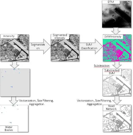
Each base map layer (buildings, road networks, and water bodies) requires a different methodological approach. The building layer extraction starts with LiDAR point cloud classification, rasterization of classified building points, vectorization, size filtering, and aggregation. The road networks is generated by using the SVM (Support Vector Machine) classifier on a segmented intensity image, DTM, and nDSM. Some data manipulation (building subtraction, vectorization, size filtering, and aggregation) still need to be applied to create more accurate and reliable road networks layer. The water-bodies layer is detected from the hole or NoData in the intensity image.
Figure 3. The building extraction methodologies
3.3.2 Road and Water bodies Extraction: A Support Vector Machine (SVM) classifier is applied to classify the Road and Non-Road class. For this purposes, the intensity image is clustered by applying segmentation based on the Mean Shift (MS) approach, which during a previous study resulted in accurate extraction. The MS algorithm is an unsupervised clustering-based segmentation which the number and the shape of the data clusters are unknown a priori (Tao and Zhang, 2007). Successive computation of the MS algorithm is started by a kernel density computation to shift each pixel image to the average of pixel in its neighbourhood and it stops when each pixels mean sequence has converged. Then, the segmentation phase starts by delineating the convergence segment. More than one hundred training areas are generated from the segmented intensity image as supervised learning for SVM classifier with 300 samples. The segmented intensity image and DTM data are used as the input data in the SVM classification. The result of the classified SVM image is then subtracted from the result of then nDSM Random Tree to remove the high objects such as buildings or trees.
Figure 4. The road and water-bodies extraction methodologies
Laser pulses are often absorbed by water, creating holes in the point cloud data or in the intensity image. This study took advantage of holes in LiDAR point clouds and the NoData values in the intensity image to classify water bodies and estimates water body boundaries. Water-bodies are reclassified from the intensity image into two classes, the NoData as water class and other value for non-water class.
Both of the SVM classified raster and the reclassified intensity image is converted into vector data based on the cell size and cell value. The size filtering is carried out by put a reasonable threshold to minimize noise. The final step is aggregating each vector data to fill in gaps inside polygons and join possible contiguous object polygons.
4. RESULT AND DISCUSSION
A visual comparison of four geospatial information features (buildings, water-bodies, road network, and contour lines) of the resulted data and reference data is shown in Figure 5.
Figure 5. Comparison the reference data (left) and the resulted data (right)
The result of this study is analysed and compared by using a 1:10.000 base map. In order to assess the quality and evaluate the accuracy of geospatial information layers resulting from this study, there are two different quantitative approach: 1. Confusion matrix (Kappa Index), 2. Completeness, correctness, and quality compare to the reference data.
4.1 Confusion Matrix (Kappa Index)
This matrix provides a cross tabulation of the class label predicted by the classification analysis against that observed in the reference data in the study area (Strahler et. al., 2006). Confusion matrix is performed by using random sampling points by considering the polygon size and shape. Therefore, different numbers of sampling points are assigned for building, road and water bodies polygons. There are three classes calculated in the confusion matrix: Buildings (B), Road Networks (R), and Water bodies (W). The present of unclassified object (U), as the additional class, is added to describe the non-detected object areas in the resulted data.
CLASS Reference Source
- Overall Accuracy: 0.713
Table 1. Confusion matrix result
Table 1. shows that Overall Accuracy (OA) of the classification result is 71.3% and it means that about 67.8% points are correctly classified and 28.7% are assigned with errors. Based on the user and producer accuracy result, the water class has the poorest accuracy and reliability (31.5%). The road network has low reliability (36.1%) but has highest accuracy (99.1%). It means that almost 91.1% of road network in the result data are correctly classified as road network but only about 36.1% of road network in the result data are correctly identified.
4.2 Completeness and Correctness
The completeness and correctness assessment is calculated based on the comparison of the area between the existed objects in the reference data and the detected objects in the data result for each layers.
There are three cases to calculate the map quality in this study:
- True Positive (TP), overlap area between the resulted and
reference data.
- False Positive (FP), object only found in the reference data. - False Negative (FN), object only found in the resulted data.
Figure 6. Definition of three different polygon cases
Each cases are applied in the equations as follows:
Branching Factor = ��/��
Miss Factor = ��/��
Completeness Percentage = ��/(��+��) * 100% Correctness Percentage = ��/(��+��) * 100% Quality Percentage = ��/(��+��+��) * 100%
Building Areas
(m²)
Road Networks
(m²)
Water Bodies
(m²)
True Positive (TP) 473629.275 295052.742 162302.929
Flase Positive (FP) 146645.188 492516.294 27539.592
False Negative (FN) 117418.976 59532.031 356755.966
Table 2. Total count of each object layer in the study area
Buildings Road
Networks
Water Bodies
Branching Factor 0.31 1.67 0.17
Miss Factor 0.25 0.20 2.20
Completeness (%) 80.13 83.21 31.27
Correctness (%) 76.36 37.46 85.49
Quality (%) 64.20 34.83 29.69
Table 3. Assessment result for different object features
The road network has highest completeness (83.21%) while the water-bodies has highest correctness (85.49%) and highest quality is achieved by building layer (64.20%).
The water bodies class have a better branching factor but a higher miss factor, which means water bodies are not easily classified but have high ability to detect the object precisely. Water bodies achieve highest correctness and it means that laser pulses, which not reflected back to the sensor accurately indicate the presence of water in the surface. In contrary, the high completeness value is achieve by road networks class but has low correctness or are mis-classified. The highest quality is achieved by building class since it has good and balance of completeness and correctness value.
4.3 Discussion
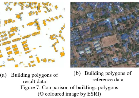
4.3.1 Buildings: There are some over-classifications of building objects since some of trees or high vegetation are classified as building points. Applying a texture-based classification should improve building classification.
(a) Building polygons of result data
(b) Building polygons of reference data
Figure 7. Comparison of buildings polygons (© coloured image by ESRI)
4.3.2 Road Networks: The similar elevation, surface texture, and intensity value might cause the inundated rice fields is detected as road surface. The example of this misclassification is shown in Figure 8.
Figure 8. Inundated rice field classified as road (© coloured image by ESRI)
One of the main reasons for the low classification result is that the road extraction algorithm mainly relies on a good segmentation. In this study, many lush trees located along the road corridor often result in a discontinuous road cluster or segment.
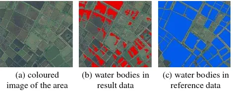
4.3.3 Water-bodies: Unidentified water-bodies in certain areas are caused by similar intensity and heights value with roads. The low statistical results is also caused by the over-classification of water bodies boundaries by human interpreter in the reference data since they use the association interpretation key. For example, some paddy fields in Figure 10. are defined as water bodies in the reference data because the human interpreter did the association with the neighbouring areas, which sometimes incorrect. Thus, the hole in LiDAR data is an accurate indicator for water bodies but more parameters needed to delineate the outline precisely.
(a) coloured image of the area
(b) water bodies in result data
(c) water bodies in reference data Figure 10. Identification of water bodies area
(© coloured image by ESRI)
5. CONCLUSION AND RECOMMENDATION
LiDAR data processing to produce large-scale base map in single GIS environment is applicable since learning classifier algorithms and other useful functions are available. The automatic processing brought in this study still become the major issues since manual work is necessary to create and delineate hundreds of training samples for SVM classification. The data quality and distribution of the samples should be well defined and they should precisely represent the data, in order to achieve better results when performing machine learning classification.
Based on the assessment result and visual data comparison to the reference data, this study was able to define the limitations and indicate possible improvements during further work. The use of optical image will reduce the misclassified building layer by separating roofs and trees using the NDVI value. It is necessary to add possible parameters (such as shape or RGB value) to extract road networks more accurately, especially to separate roads from the flooded rice fields, since these have similar intensity values, textures, and heights. The water-bodies layer needs improvement since not all ponds and lakes are detected as holes in LiDAR data. The use hydrologic modelling as well as defining the best weights and thresholds for the watershed flow parameters should improve the automatic streamline networks and riverbanks detection.
ACKNOWLEDGEMENTS
The authors appreciate for the data support by the Indonesian Geospatial Information Agency (BIG) as well as the GIS software support by the QCoherent (for LP360) and ESRI (ArcGIS, ArcPro, ArcPy).
REFERENCES
Axelsson, P., 2000. DEM Generation from Laser Scanner Data using Adaptive TIN Models. The International Archives of Photogrammetry and Remote Sensing Vol. XXXIII, Part B4/I, pp. 110-117. Amsterdam, Netherland.
ESRI website, 2016. http://desktop.arcgis.com/en
LP360 Tutorials. Geocue, http://kb.geocue.com
O’Looney, J., 2000. Beyond Maps. GIS and Decision Making in Local Government. Redlands, California, USA.
Olofsson, P., Foody, G. M., Stehman, S. V., Woodcock, C. E., 2013. Making Better Use of Acuracy Data in Land Change Studies: estimating Accuracy and Area and Quantifying Uncertainty using Stratified Estimation. Remote Sensing of Environment 129, 122-131.
Strahler, A. H., et. al, 2006. Global Land Cover Validation: Recommendations for Evaluation and Accuracy Assessment of Global Land Cover Maps. European Communities.
Tao, W., Zhang, Y., 2007. Color Image Segmentation Based on Mean Shift and Normalized Cuts. IEEE Transaction on Systems, Man, and Cybernetics. Part B: Cybernetics, Vol. 37, No. 5.
Zhang, J. X., Lin, X. G., 2004. Object-based Classification of Urban Airborne LiDAR Point Clouds with Multiple Echoes using SVM. International Symposium of Photogrammetry and Remote Sensing, Remote Sensing and Spatial Information Sciences, Volume I-3, XXII ISPRS Congress. Melbourne, Australia.
a) (a) Parking area classified as road in the result data
(b) Parking area not classified as road in reference