INCORPORATION OF UNRELIABLE INFORMATION INTO PHOTOGRAMMETRIC
RECONSTRUCTION FOR RECOVERY OF SCALE USING NON-PARAMETRIC BELIEF
PROPAGATION
J. Hollicka,∗, P. Helmholza, D. Beltona
a
Department of Spatial Sciences, Curtin University, Australia - [email protected], (petra.helmholz, d.belton)@curtin.edu.au
Commission V, WG V/4
KEY WORDS: Sensor Fusion, Belief Propagation, Photogrammetry, Barometer, GNSS
ABSTRACT:
The creation of large photogrammetric models often encounter several difficulties in regards to geometric accuracy, scale and geoloca-tion, especially when not using control points. Geometric accuracy can be a problem when encountering repetitive features, scale and geolocation can be challenging in GNSS denied or difficult to reach environments. Despite these challenges scale and location are often highly desirable even if only approximate, especially when the error bounds are known. Using non-parametric belief propagation we propose a method of fusing different sensor types to allow robust creation of scaled models without control points. Using this technique we scale models using only the sensor data sometimes to within 4% of their actual size even in the presence of poor GNSS coverage.
1. INTRODUCTION
As the number and quality of sensors increases the need to have a method of fusing this information also increases. There is cur-rently a significant amount of research into fusing multiple dif-ferent sensors, each for difdif-ferent purposes, these include reliabil-ity (Lhuillier, 2012) and reducing drift (Kerl et al., 2013). This research has resulted in several different forms of sensor fusion each with its own limitations. For instance Bayesian based meth-ods are popular, however need to have the error distributions of the sensors specified a priori (Koks and Challa, 2003). Dempster-Shaefer based methods do not require this information however struggle to deal with conflicting measurements from sensors (Ali et al., 2012), (Jøsang and Pope, 2012), (Klein, 1993).
The number of sensors available at a reasonable cost to the con-sumer is also increasing, for example the number of sensors on smart phones increasing in number and quality each year. How-ever, when compared to sensors specifically designed for naviga-tion their accuracy is lacking. Despite their lower accuracy these sensors still find uses in many applications such as orientation finding (Ayub et al., 2012), activity identification (Tundo et al., 2013) and geotagging for Structure from Motion (Crandall et al., 2013).
In this paper we present a method of fusing accelerometer, baro-metric and GNSS measurements along with images using a non-parametric belief propagation and photogrammetry. We show preliminary results with real-world data from a commodity smart phone and digital camera. In section 2 we outline belief propa-gation in both the discrete and non-parametric forms. We then describe our method in section 3 followed by some initial results and comparisons in section 4. Finally, our conclusions and out-line of intended future work is presented in section 5.
2. BELIEF PROPAGATION 2.1 Discrete Belief Propagation
Belief Propagation over discrete variables was first published by Judea Pearl in 1982 as an efficient method of solving the marginal
∗Corresponding author
probabilities inside Bayesian Tree graphs (Pearl, 1982). Since then it has proven useful on the more general cyclic graphs. How-ever, the conditions for convergence on these graphs, if indeed it does converge, are not well understood at this point (Murphy et al., 1999), (Yedidia et al., 2000) and (Yedidia et al., 2003). De-spite this, in many cases the resulting approximations are still useful (Murphy et al., 1999), (Ihler et al., 2005).
Belief propagation also has the advantage that the state of each node is dependant only on the messages coming into it. This means that once the network stabilises, if new data is inserted or a change is made. The change will flow through the network and only those nodes that receive a new and different message will change their state. Depending on the network this may mean that a significant number of the nodes do not need to redo their calculations.
One of the most important parts of belief propagation are the conditional probability functions linking the various nodes in the graph (Pearl, 1982), (Yedidia et al., 2003) as these functions de-fine the computation that will take place.
The following steps outline the general belief propagation algo-rithm (Yedidia et al., 2003):
1. Define graph structure and compatibility functions. 2. Set variables where known to their desired states.
3. During each iteration nodeisends messageMi,jto
neigh-bourj. WhereMi,j contains a set of states and the
prob-abilities that nodejwill be in those states according to the information available at nodei. Excluding the message from nodej.
4. Step 3 is repeated until either the messages no longer change or the number of allowed iterations has been reached
The messages passed between nodes are calculated using equa-tion 1 below:
Mi,j=
X
xi
φ(xi)ψij(xi, xj)
Y
∀k∈N(i)\j
WhereMij is the message from nodeitoj, φ(xi)is the
evi-dence at nodeiandψ(xi, xj)is the compatibility function
be-tween nodesiandj. In the case of discrete belief propagation this is a vector with as many elements as possible states.
When the algorithm described above has completed the final states of the nodes is calculated using the following equation:
bi=kφ(xi)
Y
∀k∈N(i)
Mki (2)
whereφandMij are defined as above andkis a constant such
that|bi|= 1.
2.2 Non-Parametric Belief Propagation
Belief propagation was initially described for discrete states, how-ever for many complex systems discretising the variables of in-terest is either infeasible or impossible. Sudderth et al. (2003) proposed a non-parametric form of belief propagation that uses Gaussian Mixture Models (GMMs) to represent the variables of interest. This avoids the problems associated with discretising the variables and allows any state space to be used.
This non-parametric form retains many of the benefits of the dis-crete belief propagation the only significant difference is that the variables are represented by probability distributions. These dis-tributions can be of any form that allows operations to be per-formed on them. One limitation of this technique is that the num-ber of kernels in each of the GMMs increases as a result of many operations. This has computational implications as the more ker-nels there are the longer the computation will take. In order to reduce this problem, Sudderth et al. (2003) propose to use Gibbs sampling to reduce the number of kernels in a GMM. This ef-fectively trades computation time for accuracy and a balance is required.
3. METHOD 3.1 Coordinate Systems
The process of fusing the different sensors requires that we main-tain a common coordinate system or transform between differ-ent systems suitable for each sensor so that we can define rela-tionships between them. We use the right handed East-North-Up (ENU) coordinate system. This has several advantages including the natural separation of height and position. This also allows us the freedom to use either a local or globally referenced coordinate system as the only difference between them is the georeferencing. This is also the same coordinate system as the Android environ-ment (Google, 2016b) which simplifies our modelling as extra transforms are not required.
When global positioning such as GNSS is used, we use the first valid coordinate as the origin and build up from there. In the case of barometric data we can lock the initial heigh to zero or set one of the known heights without requiring the other axis to be set.
We store all our orientations as(θ, φ, ρ)whereθ, φencode ’down’ and ρis the heading. We also limit each ofθ, φ, ρ to (0, π),
(0,2π)and(0,2π)respectively. We can then compute the rota-tion from a local coordinate system to a global system as shown in equation 6
combining to give a rotation of
R(θ, φ, ρ) =Rz(ρ)Ry(θ)Rz(φ) (6)
where θis the latitude where0is+zandπis−z φis longitude such that whenθ=π/2,0is+x andπ/2is+y
ρis the heading clockwise from north
Using this system of coordinates we can independently calculate up and the heading which allows certain useful cases. For ex-ample, with accelerometer data we can easily calculate the direc-tion of gravity, whereas the heading cannot be determined. Once global coordinates are introduced the heading can be determined without changing our coordinate system.
3.2 Sensor Models
The measurements from a barometer can be used in two ways, firstly to calculate an absolute height and secondly to calculate the relative height difference between two points. Currently in our work we do not attempt to calculate the absolute height as this would require a reference pressure. This reference would change over time making the calculation unreliable unless this reference is constantly updated. Instead we use the barometer to calculate relative heights between successive measurements. The calculation for relative height difference is given in equation 7 below (Engineering Toolbox, 2016):
When taking measurements from the accelerometer we generate an estimate of ’down’, allowing us to estimate the orientation of the sensor platform at each measurement using the following equations:
where Ax,Ay,Azare the accelerometer measurements
In order to resolve the ambiguity ofφwhenAx>0we set
φ= 2π−φ (10)
While we model many primitive sensors there are some sensor platforms such as digital cameras which are a combination of sen-sors and as such we construct the sensor platforms from a combi-nation of our primitive sensors. A modern digital camera records many more details that just image data, other common data may include: focal length, timestamp, geolocation from GNSS and orientation. We intend to use all of these details in future ver-sions of our fusion algorithm. When using a smart phone to log different sensors we take the latest value from the available sen-sors and tag the image with those values.
3.3 Sensor Calibration
In our work we assume that sensor measurements from the ac-celerometer and barometer can be calibrated by using a scale and offset as shown in equation 11 below and their errors modelled with a Gaussian distribution. In the case of GNSS these error dis-tributions are provided directly by the sensors otherwise are the result of calibrations.
Xc=Xu·M+O (11)
where Xuare the uncalibrated measurements
Mare the scales for each axis Oare the offsets after scaling Xcare the calibrated measurements
Accelerometers and barometers generally do not record their un-certainties, so we are required to perform a calibration in order to specify the uncertainties in our model. We then assume that this calibration is stable and holds for the whole data collection period.
For an accelerometer this calibration is performed by recording a series of measurements while the device is stationary in sev-eral different orientations. We then solve equation 11 such that
|Xc|= 9.81ms−1in order to find the scale and offset values for
each axis. We also assume that the axis of the sensors are orthog-onal, again negating the need for more complex calibrations.
For GNSS sensors we use the accuracy reported by the GNSS system to provide the variance of the Gaussian error distribution. On Android systems the error reported by the GNSS system is the standard deviation of a Gaussian distribution which fits our model (Google, 2016a).
Calibration of the barometer has been performed by recording barometer measurements for 5 minutes then computing the stan-dard deviation of the results. At this stage calibration for possible scale error is not performed as for the heights and time periods in current testing this is unlikely to be significant.
For barometers there is another step that should be performed at the time the measurements are taken for greater accuracy. In many places for the scales we are looking at the local air pressure changes significantly even in short periods of time. To combat this we record the air pressure at the beginning and end of the cap-ture period from the same point and calculate a correction factor using equation 12 below. This increases accuracy significantly.
correction(τ) =τP2−P1 t2−t1
(12)
In our calibrations at this stage we assume that the offset between the different sensors is negligible, allowing us to omit several variables from our model. However, with more accurate sensors or larger distances between them this is something we would have to take into account.
3.4 Belief Propagation Algorithm
A non-parametric belief propagation algorithm is implemented following similar principles to Sudderth et al. (2003) and Crandal et al. (2013). Each of our variables is represented as a bounded GMM with a uniform component as described in equation 13:
{µi, σ2, wi}iK=1, u,{λlower, λupper} (13)
where {µi, σ2, wi}are the mean, variance and weight of
theithkernel in the GMM
uis the uniform distribution
{λlower, λupper}are the upper and lower bounds
The use of a uniform distribution is not universal, it is not de-scribed by Sudderth et al. (2003), however Crandall et al. (2013) find that it assists with convergence when conflicting messages are present.
Many operations on GMMs increase the number of elements in the result. Which results in increased computation time. To combat this resampling methods are often used. Sudderth et al. (2003) use Gibbs sampling, whereas we use a more simple hill climbing method. We use the means of the kernels as a potential starting point. Firstly, selecting the mean with the largest value of the GMM at that point then using Newton-Raphson to refine. Using this value we calculate the variance and weight then create a new distribution in the new resulting sub-sampled GMM. This algorithm is detailed below:
1. Find the maximum of the current GMM by testing each of the internal distributions and the upper and lower bounds then use up to 10 iterations of Newton-Raphson to refine to local maximum saving the bestµandv. Whereµis the position of the maximum andvmaxis the value.
2. Ifv < thresholdthen end.
3. Setσ2to the average kernel variance in the GMM. 4. SetvarStep=σ2/2
5. Calcw=vmax
√ 2πσ2
6. err=f(x|µ, σ2)−GM M(µ+σ2)−GM M(µ−σ2) 7. If|err|< allowErrthen goto 11
8. Iferr >0
(a) thenσ2+ =varStep (b) elseσ2−=varStep
9. SetvarStep/= 2
10. Goto 5
11. Add new kernel to current GMM with{µ, σ2,−w}and new kernel to new GMM with{µ, σ2, w}.
12. Repeat from1untilKkernels are in the new GMM.
completed we combine the remaining probabilities into the uni-form distribution of the new GMM. Afterwards, we normalise the weights so that the sum of all weights and the uniform distribu-tion equals one.
This resampling is run after the calculation of message values so that the messages are both normalised and not ’too large’. In our implementation we have chosenK= 20,allowErr= 0.01and threshold= 0.001. These values are chosen as a compromise between speed and accuracy, larger values ofKand lower values ofallowErrandthresholdare more accurate but slower.
3.5 Belief Propagation Nodes
We define three different types of nodes in our implementation of belief propagation, these are constant, function and variable nodes. The constant and variable nodes are essentially the same in that they do not perform any significant processing and only maintain a value. The difference is that the constant nodes have their variable set on initialisation and thereafter it does not change whereas the value of the variable nodes changes in response to incoming messages.
The function nodes on the other hand implement various process-ing steps and in many cases also store a value. This is done to simplify the resulting graph that is created. While it would be possible to create a graph from only variable and function nodes that do not have state it would be much larger and more complex.
Our barometer nodes are functional nodes that combine both a sensor measurement and a functional node that calculates the rel-ative height change between connected nodes. Each barometer node passes its estimated height and local pressure measurement to the nodes around it. This allows the neighbouring barometer node to estimate the height difference using the pressure differ-ence and equation 7 hdiffer-ence calculating its local height. This is then combined with other height estimates passed to this node to give an estimate of the height at this node.
Our accelerometer node uses equations 8 and 9 internally to esti-mate its own orientation which is then passed as part of the out-going message along with the acceleration values measured.
We implement our image nodes as simple variable nodes that do not do any processing but just combine position and orientation estimate from connected nodes.
The last node required for this implementation is an ’Image Match’ function node. This node contains the relative orientation be-tween two images as calculated using photogrammetry. In a sim-ilar way to the barometer node outlined above this node takes the orientation of one image then provides an estimate of the orienta-tion of the other connected image. At this point this relative ori-entation is precalculated using Agisoft Photoscan (Agisoft, LLC, 2016).
3.6 Graph Generation
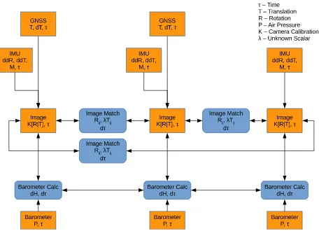
Using the nodes described above we can automatically generate a graph from a dataset of sensor measurements at run-time. At this stage we create an image node for each image and constant or function nodes from the sensor measurements as described above. These constant nodes apply the calibrations and coordinate trans-forms described above and cache the results internally so they are not recomputed at each iteration step. We then take the relative orientation of the images from another piece of software and cre-ate a set of ’Image Match’ nodes linking the images. This results in a graph similar to Figure 1 below.
Figure 1: Illustration of a section of a graph generated using our technique. Function nodes in blue and sensor measurement nodes in orange.
3.7 Scale
In order to generate a scaled and oriented point cloud we first take a set of images of the object or scene of interest with one or more sensor platforms while logging the relevant sensor information. The process is then as follows:
1. Use Photoscan to generate a point cloud and set of camera positions and orientations.
2. Run our belief propagation algorithm as defined above on the sensor data to generate a geolocation, orientation and position estimates.
3. Take the most likely value for the height and orientation of each camera
4. Rotate Photoscan point cloud using the generated rotation 5. Use least squares to translate and scale the point cloud
The coordinate system used by Photoscan is a right handed coor-dinate system where the local coorcoor-dinates for each image are such that x-y-z is down-right-backwards. To transform this into our coordinate system we apply the following transform. Firstly, we apply the inverse rotation of the first camera, then we transform to the coordinate system used by Android so that the coordinates from Photoscan match the coordinates from the Belief Propaga-tion. Finally, we apply our calculated rotation of the first camera so that everything is in our ENU world coordinate system.
˜
XEN U=R(θ, φ, ρ)
0 1 0
−1 0 0
0 0 1
R−01X˜P S (14)
where R0is the rotation of the first camera
˜
XP Sa camera location from Photoscan
˜
XEN Ua camera location in our ENU system
4. RESULTS 4.1 Sensors
Real data from a Galaxy SIII smart phone and a Canon 6D digital camera have been used to evaluate our approach. The Galaxy SIII contains a GNSS sensor which reports at approximately 1 Hz us-ing both GPS and GLONASS. It also contains an accelerometer and barometer which report at approximately 100 Hz and 25 Hz respectively. We also use the built in camera to provide image data with the camera fully zoomed out. Under the Android oper-ating system the exact reporting rate is not guaranteed, however timestamps in nanoseconds are given for each of the measure-ments. Images are not timestamped like the other sensor mea-surements, so we place a tag in the log file when an image cap-ture was triggered. Then, we assign the image the same times-tamp as the previous sensor measurement. The images captured are 8 megapixels (3264x2448 pixels). The Canon 6D records 20 megapixel (5472x3648 pixels) photographs using a 50 mm prime lens.
4.2 Calibrations
Using the calibration methods described in section 3.3 above, our calibration values for the Galaxy SIII sensors are given in Ta-bles 1 and 2. The error reported by the GNSS system for each measurement was used for the standard deviation. The average standard deviation for each sensor is recorded in Table 3 below.
Parameter Mx My Mz
Accelerometer 1.0023 0.9904 0.9888
Barometer - - 1.0000
Table 1: Calibration scales for sensors.
Parameter Ox Oy Oz
Accelerometer 0.1149 0.0889 0.5064
Barometer - - 0
Table 2: Calibration offsets for sensors.
Sensor σx σy σz
Accelerometer 0.0206 0.0198 0.0298
Barometer 7.5400
GNSS - Limestone Blocks 199.89
GNSS - War Memorial 442.07
Table 3: Sensor standard deviations after calibration
To give an idea of scale, a standard deviation for the barometer of 7.54 Pa in Table 3 results in approximately 0.63 m of elevation at the standard atmospheric pressure of 100 kPa.
4.3 Datasets
We have collected data from two areas. Figures 2 and 3 show an example image of each dataset with measurements. For the Limestone Block dataset 35 images from the 6D and 13 images from the Galaxy SIII were captured. For the War Memorial, 36 images from the 6D and 17 images from the Galaxy SIII were captured. These provided enough coverage to create a mesh of the relevant parts in Photoscan.
Neither of these datasets has full GNSS coverage with the Galaxy SIII. Only 8 of the 13 images from the Limestone Block dataset and 15 of the 17 images from the War Memorial dataset have GNSS measurements. In addition, the very large average stan-dard deviations shown in Table 3 for the GNSS suggest that the GNSS data is rather poor.
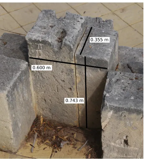
Figure 2: Illustration of the three measurements made on the war memorial dataset. Measurements numbered one to three from top to bottom.
Figure 3: Illustration of the three measurements made on the war memorial dataset. Measurements numbered one to three from top to bottom.
4.4 Accuracy
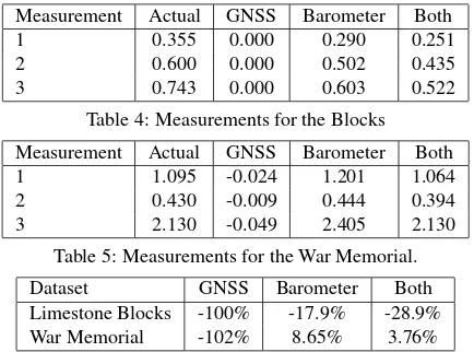
Tables 4 and 5 show the resulting measurements shown in Figures 2 and 3 after the point cloud and mesh have been scaled using the procedure in 3.7.
It is clear that using GNSS alone in this case is near useless as there is just too much error. The scales calculated for these re-sults were0.000and−0.020respectively, hence the nonsense results. However, the barometric data by itself is reasonably good and in the case of the War Memorial dataset the combination of barometric and GNSS measurements proves to be quite accurate especially given the errors of the input data.
of excluding truly bad data needs to be implemented in order to resolve this problem.
Measurement Actual GNSS Barometer Both
1 0.355 0.000 0.290 0.251
2 0.600 0.000 0.502 0.435
3 0.743 0.000 0.603 0.522
Table 4: Measurements for the Blocks
Measurement Actual GNSS Barometer Both
1 1.095 -0.024 1.201 1.064
2 0.430 -0.009 0.444 0.394
3 2.130 -0.049 2.405 2.130
Table 5: Measurements for the War Memorial.
Dataset GNSS Barometer Both
Limestone Blocks -100% -17.9% -28.9%
War Memorial -102% 8.65% 3.76%
Table 6: Percentage error for each set of sensors.
5. CONCLUSION
In this paper we present a sensor fusion method to fuse accelerom-eter, barometer and GNSS data using Non-Parametric Belief Prop-agation. Once a device is calibrated this method requires no setup, control points or extra work on behalf of the person captur-ing the data. All of the analysis and scalcaptur-ing is performed without extra input or physical measurement on the actual objects being reconstructed. This is potentially useful in several cases where access is difficult or impossible or it is not possible to touch or actively scan the objects.
While these results are preliminary the data is less than ideal sug-gesting that there is potential to get useful results even in the pres-ence of significant outliers. For example, despite the very large errors in the GNSS data we are still able to achieve results that have much less error that the input data.
5.1 Future Work
While this implementation of sensor fusion shows improvement over just using the raw sensor data there is scope for improve-ment in several ways. For example, when there are other sensors available it would be useful to attempt to automatically calibrate sensors such as the barometer using the additional data. This would remove the current method of returning to the start point which is not always possible in many situations.
In this implementation we utilise Photoscan to perform the pho-togrammetry component. This is not ideal for several reasons. At the current time the algorithms used by Photoscan are not pub-licly known which limits transparency and understanding of what causes a particular error. Secondly, with the extra information available from multiple sensors as either constraints or as initial-isation values implementation of our own or modification of an existing open source photogrammetry package would be ideal for making use of this data.
REFERENCES
Agisoft, LLC, 2016. Agisoft Photoscan. http://www.
agisoft.com(16 Apr. 2016).
Ali, T., Dutta, P. and Boruah, H., 2012. A new combination rule for conflict problem of dempster-shafer evidence theory. Interna-tional Journal of Energy, Information and Communications3(1), pp. 35–40.
Ayub, S., Bahraminasab, A. and Honary, B., 2012. A sensor fu-sion method for smart phone orientation estimation. In: Proceed-ings of the 13th Annual Post Graduate Symposium on the Con-vergence of Telecommunications, Networking and Broadcasting.
Crandall, D. J., Owens, A., Snavely, N. and Huttenlocher, D. P., 2013. Sfm with mrfs: Discrete-continuous optimization for large-scale structure from motion.Pattern Analysis and Machine Intel-ligence, IEEE Transactions on35(12), pp. 2841–2853.
Engineering Toolbox, 2016. Altitude above Sea Level and Air Pressure. http://www.engineeringtoolbox.com/
air-altitude-pressure-d_462.html(17 Apr. 2016).
Google, 2016a. Location - Android Developers.
https://developer.android.com/reference/android/
location/Location.html#getAccuracy()(12 Apr. 2016).
Google, 2016b. Sensors Overview - Android
Develop-ers. https://developer.android.com/guide/topics/
sensors/sensors_overview.html#sensors-coords (12
Apr. 2016).
Ihler, A. T., Iii, J. and Willsky, A. S., 2005. Loopy belief propa-gation: Convergence and effects of message errors. In:Journal of Machine Learning Research, pp. 905–936.
Jøsang, A. and Pope, S., 2012. Dempsters rule as seen by little colored balls. Computational Intelligence28(4), pp. 453–474.
Kerl, C., Sturm, J. and Cremers, D., 2013. Robust odometry esti-mation for rgb-d cameras. In:Robotics and Automation (ICRA), 2013 IEEE International Conference on, IEEE, pp. 3748–3754.
Klein, L. A., 1993. Sensor and data fusion concepts and ap-plications. Society of Photo-Optical Instrumentation Engineers (SPIE), Bellingham, WA, USA, 131 p.
Koks, D. and Challa, S., 2003. An introduction to bayesian and dempster-shafer data fusion. Technical report DSTO-TR-1436,
35 p., http://dspace.dsto.defence.gov.au/dspace/
bitstream/1947/4316/5/DSTO-TR-1436%20PR.pdf.
Lhuillier, M., 2012. Incremental fusion of structure-from-motion and gps using constrained bundle adjustments. Pattern Anal-ysis and Machine Intelligence, IEEE Transactions on 34(12), pp. 2489–2495.
Murphy, K. P., Weiss, Y. and Jordan, M. I., 1999. Loopy belief propagation for approximate inference: An empirical study. In:
Proceedings of the Fifteenth conference on Uncertainty in arti-ficial intelligence, Morgan Kaufmann Publishers Inc., pp. 467– 475.
Pearl, J., 1982. Reverend Bayes on inference engines: A dis-tributed hierarchical approach. In:AAAI, pp. 133–136.
Sudderth, E., Ihler, A., Freeman, W. and Willsky, A., 2013. Non-parametric belief propagation. In: In IEEE Computer Society conference on computer vision and pattern recognition (CVPR), Vol. 1, pp. 605–612.
Tundo, M. D., Lemaire, E. and Baddour, N., 2013. Correct-ing smartphone orientation for accelerometer-based analysis. In:
Medical Measurements and Applications Proceedings (MeMeA), 2013 IEEE International Symposium on, IEEE, pp. 58–62.
Yedidia, J. S., Freeman, W. T. and Weiss, Y., 2000. Generalized belief propagation. In:NIPS, Vol. 13, pp. 689–695.