VECTORIZATION OF ROAD DATA EXTRACTED FROM AERIAL AND UAV IMAGERY
Dimitri Bulatov, Gisela H¨aufel, Melanie Pohl
Fraunhofer IOSB, Department Scene Analysis, Gutleuthausstr., 1, 76265, Ettlingen, Germany {dimitri.bulatov,gisela.haeufel, melanie.pohl}@iosb.fraunhofer.de
Commission III, WG III/4
KEY WORDS:Curvature, Classification, Road datbases, Thinning, Topology, Vectorization
ABSTRACT:
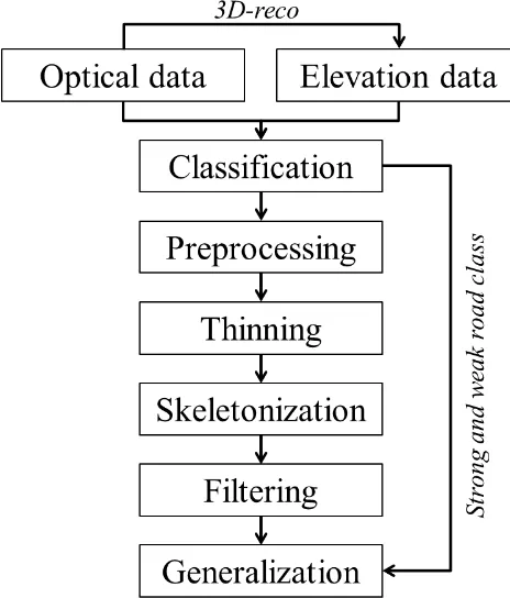
Road databases are essential instances of urban infrastructure. Therefore, automatic road detection from sensor data has been an important research activity during many decades. Given aerial images in a sufficient resolution, dense 3D reconstruction can be performed. Starting at a classification result of road pixels from combined elevation and optical data, we present in this paper a five-step procedure for creating vectorized road networks. These main five-steps of the algorithm are: preprocessing, thinning, polygonization, filtering, and generalization. In particular, for the generalization step, which represents the principal area of innovation, two strategies are presented. The first strategy corresponds to a modification of the Douglas-Peucker-algorithm in order to reduce the number of vertices while the second strategy allows a smoother representation of street windings by Bezir curves, which results in reduction – to a decimal power – of the total curvature defined for the dataset. We tested our approach on three datasets with different complexity. The quantitative assessment of the results was performed by means of shapefiles from OpenStreetMap data. For a threshold of 6 m, completeness and correctness values of up to 85% were achieved.
1. INTRODUCTION AND RELATED WORK For a large number of both civil and military applications, roads are an essential part of urban infrastructure. Hence, their de-tection and modeling represent an important step on the seman-tic reconstruction process of urban terrain in combined opseman-tical and elevation sensor data. However, especially in urban envi-ronment, extraction of road networks from airborne sensor data is a challenging task. The main challenges are made up by the variety of appearances and road types (sidewalks, tunnel entries, bridges, railways, etc.), occlusions (tree crowns or moving ve-hicles), shadows, and many others. In particular for the case of elevation maps obtained from aerial images via multi-view dense matching (Hirschm¨uller, 2008, Rothermel et al., 2012), outliers in street areas which are caused by moving objects and homoge-neous road texture are often present.
From the extensive surveys, such as (Mena, 2003), different strate-gies for extraction of roads from the available sensor data can be adopted. In the case that an initialization of the vector representa-tion for the road network is available, fully-automatic approaches to improve its geometrical correctness by means of snakes whose data term is calculated from the input images (Butenuth and Heip-ke, 2012) and even 3D laser point clouds (Boyko and Funkhouser, 2011) were proposed. In (Klang, 1998, Turetken et al., 2013), po-sitions of road junctions are detected and used as seed points for an active contour model or as graph nodes. The connections be-tween graph nodes can be determined by searching tubular struc-tures in (Turetken et al., 2013) in 2D or 3D data, after which the topology is modified within a non-local optimization process. However, it remains not always clear what happens to geome-try (smoothing curvilinear segments, dealing with their intersec-tions, etc.). Regarding structurally-coherent soluintersec-tions, (Chai et al., 2013) introduce a method for line-network recovering in im-ages by modeling junction point processes. The approaches of (Hinz and Baumgartner, 2003, Hinz, 2004) already permit a rep-resentation of road nets as 2D polygons (level of detail 2). In the first approach, lines obtained from the images and elevation data are grouped into stripes. Finally, road segments and whole
net-works for roads are iteratively obtained from these stripes. The second approach is a sophisticated scale- and context-dependent procedure in which typical relationships between different object classes are exploited. If one is interested in extraction and vec-torization of the centerlines of roads, three main strategies can be observed.
smooth curve is aimed, and (Noris et al., 2013), where minimal spanning trees of points near the centerline are analyzed; these points on the centerlines are obtained by clustering of salient (e.g. with respect to their gradient) pixels. In (Mena, 2006), starting from the binary imageRrepresenting road pixels, the road cen-terlines are supposed to have the same distance to at least two points ofR. This method is very sensitive to the classification results. Every concavity inRleads first to short, superfluous seg-ments and, additionally, to zigzag-like, improbable street courses. The first way to improve the performance is to put some effort for a better classification result. However, working with 2D regions in a non-local optimization process is computationally expensive. Additionally, even the pioneering approach on road classification, stemming from (Wegner et al., 2015), cannot prevent that in final result, some trees occlude parts of roads. Because of these two reasons, the second way, namely, a post-processing routine of the remaining roads appears to be a promising method.
In this paper, we propose a vectorization procedure for extraction of road networks from a binary road class map. The vectorization procedure is somehow similar to (Miao et al., 2013), but its main focus lies on post-processing of the results of thinning. During an iterative filtering step, all branches of the skeleton are ana-lyzed on their necessity and relevance. The unnecessary branches are evidently deleted. Afterwards, in a generalization step, two strategies are proposed: first, we consider a modification of the algorithm (Douglas and Peucker, 1973). The modified algorithm rectifies the line courses, however performs an additional check to force the rectification to traverse the segmentation results of road class. Within the second approach, the high curvature and ragged course of roads is reduced by performing a transforma-tion of roads into (ratransforma-tional) Bzier curves under consideratransforma-tion of the segmentations for road class. The Bzier curves are discretized to retrieve the correspondence with the road segments.
The paper is structured as follows: in Sec. 2, we refer to the pre-liminaries on extraction of (N)DSM, DTM, as well as classifica-tion results since this knowledge is important to understand our vectorization algorithm, which will be given in Sec. 3. The post-processing of the resulting road net will be covered in Sec. 4. We show in Sec. 5 computational results for three datasets and give a summary and some ideas for future work in Sec. 6.
2. PRELIMINARIES
Aerial and even UAV-images are a very suitable input for an urban terrain reconstruction procedure. The resolution of such images is rather high compared to airborne laser point clouds and the problem of occlusions is mitigated by means of many redundant views. First, image orientation is performed by a state-of-the-art method, e.g.Bundler, (Snavely et al., 2010). Then, computation of a 3D point cloud and finally, creation of a DSM (digital surface model) and an orthophoto takes place by the dense reconstruction pipeline (Rothermel et al., 2012). From DSM, the ground model, also denoted as digital terrain model (DTM), is obtained by the procedure (Bulatov et al., 2014a), Sec. 2.1. The difference be-tween DSM and DTM is denoted as NDSM (normalized DSM).
Two different classification methods as basis for our vectoriza-tion procedure are explained in the following. First, subdivision of terrain into several classes (building, tree, grass area, and road) is performed by a procedure similar to that described in (Lafarge and Mallet, 2012). Several measures – relative elevation, pla-narity, normalized difference vegetation index (NDVI), satura-tion measure, and entropy – are computed for each pixel. The first two measures are applied on the NDSM while the three lat-ter measures are applied on the orthophoto. Note that in order
to mark vegetation pixels, the green channel can be taken instead of the near infrared color for computing NDVI. Hence, trees in shadows tend to belong to the building class while the grass areas in shadows tend to belong to the road class. Then, these mea-sures are collected into energy data terms for all classes. For example, the data term for road pixels should combine a low NDSM and NDVI value, while planarity and saturation values should be high. A smoothness term penalizing differences of la-bels between neighboring pixels is added to the energy function for which a strong local minimum is found using a non-local op-timization method, such as (Hirschm¨uller, 2008). The resulting label map is post-processed by the median filter. Unfortunately, the classification results have several short-comings. First, there are further objects that are rarely to find in the dataset (earth hills, vehicles, street-lamps, fences, etc) and which, in general, cannot be easily assigned to the “clutter” class of (Lafarge and Mallet, 2012). Second, the linear truncated function, originally applied to convert the measures into the data term, was not suitable for our problem and was replaced by a sigmoid-like function asymp-totically approaching 0 and 1. However, the parameters of such a function are not always easy to choose since they often vary over the terrain and should better be subject of a training procedure.
Recently, a pioneering approach for extraction of road pixels from an orthophoto, optionally supported by an elevation map, was proposed by (Wegner et al., 2015). The main innovation of this approach is a global minimization of an energy function with an asymmetric smoothness term. This term heavily exploits the fact that the probability that a path ofN≫2 patches of a classAis interrupted by a path of the complementary class (notA) is ex-tremely low ifAis the road class. The approach consists of four main steps. In the first step, image segmentation into superpixels is performed. This is done for compression of image informa-tion. It is a balance act between keeping the output as rectangular grid structure and preserving boundaries between the objects in the image. In the second step, the data cost, that is, the like-lihood of a superpixel to belong to the class road, is specified using predefined filter banks and elevation information. In the third step, minimum cost paths are formed between superpixels of very low data cost. This is done in order to identify poten-tial roads even though a little number of paths’ superpixels is oc-cluded and therefore exhibits high data energy. These paths are input of the non-local optimization based on Conditional Random Fields (CRFs) which makes up the fourth, final step of the proce-dure. The penalty term for such a path is high if it is interrupted by superpixels belonging to the classnon-road. A conventional, symmetric 2-clique term penalizing differences of classes of ad-jacent superpixels is added as well. Because there are only two classes, optimization on such CRF with graph cuts yields a global minimum of the energy function in a reasonable time.
The method performs rather well in identifying the road class, and its short-comings mostly result from the NDSM which was computed by a local method. There are also some trees straddling into the road class and sometimes occluding very narrow paths. However, even this excellent classification needs a vectorization for road representation in most visualization and simulation soft-ware applied for city modeling tools, urban planning, training and simulation of rapid response tasks, and many others. The problem of road vectorization, that is, converting road pixels into 1-dimensional shapefiles (polylines, level of detail, LOD1) will be the topic of the following section.
Rrepresenting the road class is performed by means of morpho-logical operations followed by filling small holes inR(mostly, left by cars) and deleting small isolated segments ofR. This is done by applying acleanfilter – that is, labeling and suppress-ing regions of too small areas – first on the complement ofRand then, on the imageRitself. In the second step, we perform thin-ning, that is morphological skeletonization of the resulting image
¯
R. As a result, the new binary image is created where only pixels belonging to the medial axis are set to one. After this, these pix-els are collected into a set ofpolylinesusing thepolygonization method (Steger, 1998). However, every concavity and protrusion of the binary imageRreflects in a polyline which leads to a high number of short polylines and, since we wish every polyline to represent a road segment, to a very noisy and barely plausible road network. Consequently, the fourth step of our vectorization routine,filtering polylines, will be described in the remainder of the section while the final step, generalization, will be explained in Sec. 4.
Figure 1: Filtering polylines. Top: assessing segments and junc-tions, bottom: updating topology. See text for more details.
Note that in general, it is not enough to filter out short road seg-ments because some of them may connect to other polylines or bear other important functionality. Together with the geometry, the topology of every polyline as a part of the road net is relevant. In most applications, too short dead-end (terminal) roads are un-necessary and should be deleted. Therefore we calculate for ev-ery polyline not only geometry attributes, like length, width, and principal direction, but also topological properties. By comput-ing nearest neighbors for every endpoint of the road, and assess-ing the number of neighbors within the distance of one pixel, we decide whether a putative road endpoint is a terminal one or be-longs to exactly onejunction. For every junction, we store its approximate position, theactivity statusas well as the three road segments incident with it in an additional array. At the begin-ning, all junctions are set active. As for calculation of geometric attributes for polylines, we determine the length, the dominant di-rection of a road, as well as its approximate width. The dominant
direction results from the principal component analysis (PCA) of the vertices forming the course of a road. The first principal component determines the vector of the dominant directionuof a road while the second (perpendicular) directionu⊥is used to de-termine the road width. For each vertex of a road, we measure the mean width of both rays starting at it and running parallel tou⊥ that lie in the segmentation result using the algorithm of (Bresen-ham, 1965). The weighted average of these values yields the total value of the road width. To exclude invalid values of widths as it happens at roads on the image boundary or big plazas, we ignore single-vertex widths below or above predefined values (1 m and 40 m). It must be stated that the determination of the dominant direction by means of PCA does not make much sense for arc-shaped roads. Thus, also the width values for this kind of roads may become incorrect; hence, stabilizing of road width computa-tion will be part of our future work.
The geometry of a putative road segment is defined to be reli-able if the width is bounded between two thresholds (around 3 m and 30 m in urban scenes) and the length exceeds 5 m. These thresholds depend on the definition of what a road segment is which is mostly given by the application. For example, it does not make sense to include the short ways between house entries and main streets into any road database. In a different example, a large parking lot, especially with several trees, provides a large number of road segments which are not necessary. Since we are interested in eliminating the short terminal segments, we define the topology of a putative road object to be reliable if its both ends are incident with an active junction.
The iterative filtering procedure of road objects includes two mod-ules. In the first module, all road segments which are not reliable both with respect to geometry and topology are set inactive. At the same time, all junctions with less than three active incident roads are declared inactive. In the second module, we update the geometry and the topology. All inactive road segments and junctions are deleted. However, for all inactive junctions with ex-actly two active incident polylines, these segments are merged, and their geometric and topological attributes are recalculated. It is clear that already the first module can be implemented as an iterative procedure. However, the number of its subsequent applications must be small, because without a regular update of geometry and topology, good roads may become partly deleted (for example, in Fig. 2, without updating geometry and topology, first polylines 1, 2, 4, and 9, and finally, the polyline 3 would be deleted). The remaining active road segments represent the output of our vectorization procedure.
4. GENERALIZATION
After the superfluous parts of the medial axis have been deleted, the main problem is the course of the remaining roads. It is of-ten wriggled as a consequence of objects bordering and overlap-ping roadsides. For example, there could be convexities caused by pavements spuriously added to the road class and concavities caused by trees occluding roads. Some problems can be miti-gated by morphological operations; however, the resulting mask of road areas still remains ragged. The particular difficulty of any straightening method is that it is not easy to establish a cost func-tion and hence to assess the quality of a putative improvement. Theoretically, it is clear that straight road courses are desirable; so are right angles in the junctions. However, not in all situations, these improvements are correct. We present two strategies for generalization of road segments previously obtained. In Sec. 4.1, the modified Douglas-Peucker algorithm will be explained while in Sec. 4.2, we present the method based on approximating poly-lines by Bzier curves.
4.1 Generalization Based on the Modified Douglas-Peucker Algorithm
The key idea of the method (Douglas and Peucker, 1973) is to bi-sect recursively the polylineP={p1,p2, ...,pn}. We first obtain the furthest vertex from the edge connecting the endpoints ofP:
d=dj=max
i (kpi,p1pnk), j=arg maxi (kpi,p1pnk). (1)
Ifddoes not exceed a thresholddmax, the generalization is con-cluded by connectingp1and pn. Otherwise after bisection, the same procedure is applied on the two partial polylines{p1,p2, ...,pj} and{pj,pj+1, ...,pn}. This algorithm is rather fast and it is global since it starts by considering first the whole polyline and subse-quently narrowing the search range. This can also be a disad-vantage of the method. Deleting – without a previous check – a large amount of points in the polyline can lead to problems, such as topological inconsistencies and – in particular, for our task to determine road courses – connecting vertices penetrating an ob-stacle. Therefore, the classification result should be considered additionally to the distance betweenpjandp1pn. We consider a thin rectangleUover the straight linep1pnand check to which extend – compared to its total area –Ubelongs to the road class. The width ofUcorresponds to the safety distance from the road centerline to the non-road class. In order to narrow the search ranges forx∈U, an image fragment corresponding to the bound-ing box ofPshould be considered for further computation. Now, for a second thresholdtmin, 0≤tmin≪1, the generalization takes place if and only if 0.5 m, respectively. The first, intuitive choice of the weightsc(x) could be one if the class of the pixelxis road class and zero other-wise. However, in this second criterion,c(x)can be modified for the case we have a classification result not only for the class road, denoted asstrong road class, but for other classes, targeting full urban terrain reconstruction. We can assume that a road segment could partly pass under a tree or a large vehicle, and denote the tree and vehicle class as aweak road class, however not under the grass area or a building. A possible weight function
c(x) =
can be further improved in the future, by computing approximate tree crowns positions by means of a state-of-the-art algorithm, (Eysn et al., 2015), extracting information about gates in build-ings, etc.
4.2 Generalization Based on the Curvature of Road Seg-ments
The idea of the second, alternative generalization module is to ob-tain smoother routes, by approximating the course of every road segmentP={p1,p2, ...,pn}by Bzier curves. The curves are able to represent the road course itself and furthermore to smooth their routes. The Bzier curve is discretized atlequidistant points while lshould be big enough to guarantee a smooth outline but suffi-ciently small to be in the order of the elements of the road polyg-onal chain. We takel=max(n,11)as suitable. All points are equally weighted at the beginning. Each discretized Bzier curve is a new polygonal chainB={b1,b2, ...,bl}. IfBruns through a “forbidden area”, which can be the complement of either the strong or the weak road class as defined in the previous section, we first determine the edgesej=bjbj+1ofBthat traverse this area by means of the Bresenham algorithm. For each such edge, we compute its midpointmjand determine theknearest neigh-bors ofmjamong{p2, ...,pn−1}. The number of these neighbors
is bounded byk≤3 because three is the minimum number of ver-tices needed to form a turn. The reason to take only inner neigh-bors is that the positions of endpoints of a road segment remain unchanged by the Bzier curve. Finally, we increase the weight-ing of the determined nearest neighbors ofmiby one and repeat these steps until the rational Bzier curve ofPno longer penetrates the “forbidden area”. Note that the positions of junctions remain fixed – since they are endpoints of single polylines – and hence, there is no need to adjust the neighboring road segments.
5. RESULTS 5.1 Datasets and Qualitative Assessment
The first dataset we processed was a DSM sampled from 647 frames of the UAV-borne video sequence over the village Bonn-landin Southern Germany. The orientation of these frames was performed by means of the Bundler software (Snavely et al., 2010) while the computation of the 3D point cloud and DSM is based on the SURE software described by (Rothermel et al., 2012) with modifications indicated in (Rothermel et al., 2014). The reso-lution of this dataset was around 0.1 m and an area of about 0.6×0.2 km2was covered; (the relevant information for this and other datasets is noted in Table 1). Because the effect of shad-ows was mitigated by using a high amount of input images and by not very high buildings, the extraction of pixels of the road class was a result of threshold decision (by NDSM and NDVI value). The shortcomings of this data are the pathways around the roads, which are separated by thin walls of around 0.5 to 1 m height. Some of these walls were not reconstructed during DSM extraction, others were filtered out through the preparation step of Sec. 3.
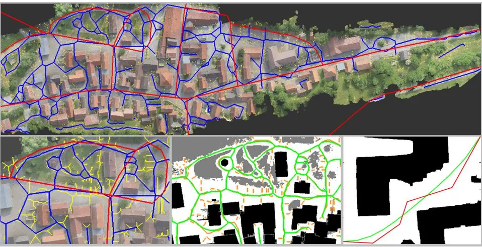
Figure 3: Results for the datasetBonnland. Top row: road segments drawn into the orthophoto. Bottom row: detailed result plotted into the orthophoto (left) and the corresponding fragment for the classification mask (black: building class, white: road class, gray: remaining pixels, middle). Bottom right, another example for the method based on Bzier curves. See text for more details.
The third dataset is a part of the inner city ofGraz, Austria. It was provided by the authors of (Wegner et al., 2015) together with classification results. The road class was extracted very accurately, therefore many short road segments were built dur-ing the computation of the skeleton. While the short terminal segments were successfully eliminated during our filtering pro-cedure, the loops built small obstacles, could not be completely avoided. Since these loops are usually not needed for the road databases, the future approach should include recognition of the content of these loops followed by the suitable generalization.
We show in Figs. 3, 4 and 5 the resulting road nets obtained by our procedure for the datasetsBonnland, GrazandMunich, re-spectively. In all these images and subimages, yellow + orange, blue and green polylines represent the results after applying the algorithm steps of Secs. 3, 4.1, and 4.2, respectively. Dashed lines always denote the polylines discarded in the filtering step of Sec. 3. Red polylines in Fig. 3 denote the road maps obtained from the free geographic data.
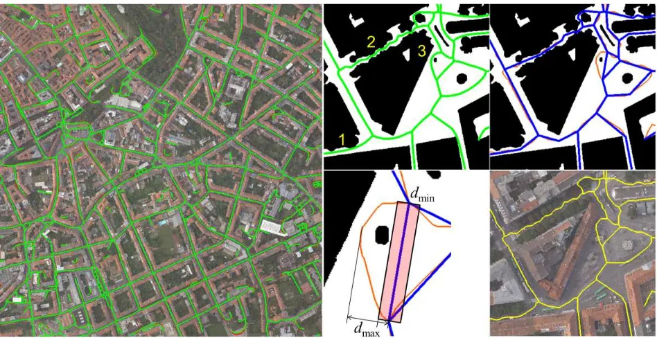
As we can see in Figs. 3-5, using Bzier curves as approxima-tion for the initial road segmentsRleads to much smoother road courses. However, this happens at cost of increasing number of street vertices. The method works locally; it does not degrade the visual result even in the case of incorrect positions of junctions, small, non-oversmoothed obstacles, etc. In the image bottom right of Fig. 3 as well as for the most straight streets in the datasets GrazandMunich, the jagged road course can be smoothed very well. However, as shown in Fig. 4, situation 1, the resulting roads can come up arbitrarily near to the forbidden areas if no care is taken (for example, by morphological operations). Thus, this method is more susceptible to the positions of junctions. On the contrary, the generalization based on the modification of (Dou-glas and Peucker, 1973) produces a strong compression of results abiding, at the same time to the classification result. This can be seen in situation 2 of Fig. 4, where the actually straight, but partly occluded by trees, segment was kept straight as much as possible by modified procedure of (Douglas and Peucker, 1973). How-ever, as one can see in the case of the small obstacle in Fig. 4,
situation 3, if the choice ofdmaxin Sec. 4.1 is too generous, the topology of the road network is slightly changed; it depends on the applications if such a generalization is desired. It can be concluded that the method based on Bzier curves has its main advantage in the case of winding streets, while the modification of (Douglas and Peucker, 1973) performs especially well for the long polylines affected by noise.
5.2 Quantitative Evaluation
The focus of the quantitative evaluation of street networks is two-fold. First, we wish to see the overlap of our result with the ground truth data, and second, the effects of the generalization shall be shown. With respect to the first goal, geo-referenced OpenStreetMap(OSM) data were selected as our ground truth and transformed into the coordinate system of the datasets. For the datasetMunich, a geo-referencing transformation was avail-able while both other datasets were geo-referenced interactively. The typical geometric measures for the quality of estimated poly-lines arecompletenessandcorrectness.
Figure 4: Results for the datasetGraz. Left: road segments drawn into the orthophoto. Top row, middle and right: detailed view of the results of two generalization methods superposed with the classification mask. Bottom row, middle: Functionality of modified procedure (Douglas and Peucker, 1973) in situation 3. Right: results of vectorization procedure superposed with the orthophoto.
Table 1: Results on correctness, completeness (fort= 60 pixels), and generalization performance for all three datasets. In the second row: resolution, area covered in km2, number of polylines, and number of streets in the shapefile for each dataset.
Dataset: Bonnland Graz Munich
Properties: 0.1,0.2×0.6,213,11 0.25,0.25×0.25,923,1173 0.2,0.95×1.2,720,977
Gen. method None DPm Bz None DPm Bz None DPm Bz
n(P|comp conf) 61 62 64 788 794 788 663 667 660
q(P|comp conf) 0.24 0.25 0.30 0.88 0.89 0.89 0.91 0.92 0.91
n(S|part conf) 11 11 11 976 960 962 685 666 670
q(S|part conf) 0.85 0.85 0.85 0.81 0.79 0.80 0.73 0.71 0.72
∑n 2496 827 3074 12626 2615 15627 8164 2091 10955
¯
κ, in◦ 238 54 55 358 30 60 231 31 59
to this measure, the sum of the lengths of confirmed edges di-vided by the sum of lengths of all shapefile segments is denoted asq(S|part conf)and shown in Table 1.
As for the second goal, since both position and activity status of junctions do not change, there are no alterations in the topology and theglobalgeometry. Thus, changes in completeness and cor-rectness between the original and generalized road networks are not significant enough. Since the generalization affects thelocal geometry, its changes can and should be tracked. While the gen-eralization algorithm of Sec. 4.1 aims to reduce the total number of vertices, this parameter – denoted by∑n– will be reported in Table 1. For the smoothing routine described in Sec. 4.2, the goal was to minimize thecurvatureof the output road segment. Hence, our second measure ¯κ is the average number of curva-turesκ(P)over all polylines. The curvatureκ(P)of a polygon P={p1,p2, ...,pn}is defined, according to (Milnor, 1950), by the sum of anglesαibetween the straight-forward direction of a polygon edge pi−1piand its successor pipi+1for all inner
ver-From Table 1, we see that the most important completeness mea-sure is roughly the same for all datasets. It is slightly higher for the datasetBonnland, since it is a simple dataset of a rural region, with eleven main roads to be confirmed. As a consequence, the values for correctness suffer (see next paragraph). The results for the datasetGraz, with its highly complicated road system, are of almost the same completeness but much higher correctness. It could further be observed that by decreasing the thresholdt, the completeness ofBonnlanddata falls below that ofGraz: build-ings further away from the roads contribute to a more wriggling course. Overall, the main explanation for the differences is that only forGrazdata, the classification result was computed with the one of the best state-of-the-art approaches on road data clas-sification. Further, minor reasons are: uncertainties in the geo-referencing, differences in resolution, and the errors in shapefiles, often present in urban data. Especially it could be observed for theMunichdata, in which, additionally, many shapefile streets close to buildings were not confirmed.
The measure for correctness is biased mainly because the def-inition of street is not explicit; especially in the dataset Bonn-land, merely main roads are contained in the shapefile. However, especially for quick response applications, the sideways, secret paths for persons and vehicles, etc., are of essential importance and should not be suppressed. Besides, uncertainties in the geo-referencing of both shapefiles and sensor data processing results affects negatively both completeness and correctness. In our pre-vious work (Bulatov et al., 2014b), the road networks from free geographic data, sensor data evaluation results, as well as super-position of both, were analyzed for the datasetBonnlandfirst by the statistical reasoning approach based on Dempster and Shafer theory (Ziems, 2014) and finally by interactive analysis of both incorrectandunknownsegments, see (Bulatov et al., 2014b), us-ing the textured urban terrain model. Through the automatic ver-ification step, there were many unknown segments (since they exhibit too high curvature or are too short compared to standard GIS roads). The interactive verification step indicated thatall questioned segments correspond to valid paths in the dataset.
Finally, we have seen that the average curvature of all streets can be reduced by a decimal power by applying the modified algorithm of (Douglas and Peucker, 1973) and the generaliza-tion method based on Bzier curves. These produce a slightly in-creased number∑nof vertices while the former method reduces
∑nto a value of 20 to 25 % without affecting much the course of the roads.
6. SUMMARY AND FUTURE WORK
We presented a fully automatic approach for the road vectoriza-tion and generalizavectoriza-tion. Starting from the sensor data, a binary image reflecting classification results is first obtained. During vectorization, a geometrically and topologically consistent road network could be created while during the generalization step, we succeeded to reduce the total curvature and the number of ver-tices. To do this, two modules were introduced: a modification of the approach (Douglas and Peucker, 1973) and Bzier curves. Both of these procedures are forced to adhere to the classifica-tion result. However, a differentiaclassifica-tion between the strong and the weak road classes have been made: the former was used for road detection and the latter for extending search range during the generalization. We have seen that the quality of road networks de-pends on the classification result: the asymmetric approach due to (Wegner et al., 2015) has yielded better, stabler results than those based on threshold decision or a symmetric classification similar to (Lafarge and Mallet, 2012). A more extensive analysis for clas-sification methods and their parameters for a fixed dataset should follow. As for vectorization, the major short-comings lie firstly in the unnecessary loops and, finally, in the unchanged, often unfa-vorable positions of junctions, whose simultaneous optimization with considering rectangularity and cardinalities of convergent streets should be considered in the future.
ACKNOWLEDGEMENTS
We express our gratitude to Mathias Rothermel from the Institute of Photogrammetry in Stuttgart for providing us the DSM data forBonnlandandMunich. The DSM and the orthophoto were computed from registered images by means of the SURE soft-ware (Rothermel et al., 2012). We further express our gratitude to Jan-Dirk Wegner for providing the input data and the results of the road detection algorithm (Wegner et al., 2015) for the dataset Graz.
REFERENCES
Boyko, A. and Funkhouser, T., 2011. Extracting roads from dense point clouds in large scale urban environment.ISPRS Journal of Photogrammetry and Remote Sensing66(6), pp. 2–12.
Bresenham, J. E., 1965. Algorithm for computer control of a digital plotter. IBM Systems journal4(1), pp. 25–30.
Bulatov, D., H¨aufel, G., Meidow, J., Pohl, M., Solbrig, P. and Wernerus, P., 2014a. Context-based automatic reconstruction and texturing of 3D urban terrain for quick-response tasks. ISPRS Journal of Photogrammetry and Remote Sensing93, pp. 157– 170.
Bulatov, D., Ziems, M., Rottensteiner, F. and Pohl, M., 2014b. Very fast road database verification using textured 3D city models obtained from airborne imagery. In:Proc. SPIE Remote Sensing, International Society for Optics and Photonics.
Butenuth, M. and Heipke, C., 2012. Network snakes: graph-based object delineation with active contour models. Machine Vision and Applications23(1), pp. 91–109.
Clode, S., Rottensteiner, F., Kootsookos, P. and Zelniker, E., 2007. Detection and vectorization of roads from lidar data. Pho-togrammetric Engineering & Remote Sensing 73(5), pp. 517– 535.
Douglas, D. H. and Peucker, T. K., 1973. Algorithms for the reduction of the number of points required to represent a dig-itized line or its caricature. Cartographica: The International Journal for Geographic Information and Geovisualization10(2), pp. 112–122.
Eysn, L., Hollaus, M., Lindberg, E., Berger, F., Monnet, J.-M., Dalponte, M., Kobal, M., Pellegrini, M., Lingua, E., Mongus, D. et al., 2015. A benchmark of lidar-based single tree detection methods using heterogeneous forest data from the alpine space. Forests6(5), pp. 1721–1747.
Gerke, M. and Heipke, C., 2008. Image-based quality assess-ment of road databases. International Journal of Geographical Information Science22(8), pp. 871–894.
Hinz, S., 2004. Automatic road extraction in urban scenes and beyond. International Archives of Photogrammetry and Remote Sensing35(B3), pp. 349–354.
Hinz, S. and Baumgartner, A., 2003. Automatic extraction of ur-ban road networks from multi-view aerial imagery. ISPRS Jour-nal of Photogrammetry and Remote Sensing58(1), pp. 83–98.
Hirschm¨uller, H., 2008. Stereo processing by semi-global match-ing and mutual information.IEEE Transactions on Pattern Anal-ysis and Machine Intelligence30(2), pp. 328–341.
Hu, X., Li, Y., Shan, J., Zhang, J. and Zhang, Y., 2014. Road cen-terline extraction in complex urban scenes from lidar data based on multiple features. IEEE Transactions on Geoscience and Re-mote Sensing52(11), pp. 7448–7456.
Klang, D., 1998. Automatic detection of changes in road data bases using satellite imagery. International Archives of Pho-togrammetry and Remote Sensing32, pp. 293–298.
Lafarge, F. and Mallet, C., 2012. Creating large-scale city models from 3D-point clouds: a robust approach with hybrid representa-tion.International Journal of Computer Vision99(1), pp. 69–85.
Mena, J. B., 2003. State of the art on automatic road extraction for GIS update: a novel classification. Pattern Recognition Letters 24(16), pp. 3037–3058.
Mena, J. B., 2006. Automatic vectorization of segmented road networks by geometrical and topological analysis of high resolu-tion binary images. Knowledge-Based Systems19(8), pp. 704– 718.
Miao, Z., Shi, W., Zhang, H. and Wang, X., 2013. Road center-line extraction from high-resolution imagery based on shape fea-tures and multivariate adaptive regression splines. IEEE Trans-actions on Geoscience and Remote Sensing10(3), pp. 583–587.
Milnor, J. W., 1950. On the total curvature of knots. Annals of Mathematics52(2), pp. 248–257.
Noris, G., Hornung, A., Sumner, R. W., Simmons, M. and Gross, M., 2013. Topology-driven vectorization of clean line drawings. ACM Transactions on Graphics (TOG)32(1), pp. 4.
Rothermel, M., Haala, N., Wenzel, K. and Bulatov, D., 2014. Fast and robust generation of semantic urban terrain models from UAV video streams. In:Proc. International Conference on Pat-tern Recognition, pp. 592–597.
Rothermel, M., Wenzel, K., Fritsch, D. and Haala, N., 2012. Sure: Photogrammetric surface reconstruction from imagery. In: Proc. LC3D Workshop, pp. 1–9.
Snavely, N. et al., 2010. Bundler: Structure from motion (sfm) for unordered image collections.Available online: phototour. cs. washington. edu/bundler/, 15 Apr. 2016.
Steger, C., 1998. An unbiased detector of curvilinear structures. IEEE Transactions on Pattern Analysis and Machine Intelligence 20(2), pp. 113–125.
Turetken, E., Benmansour, F., Andres, B., Pfister, H. and Fua, P., 2013. Reconstructing loopy curvilinear structures using integer programming. In: Proc. IEEE Conference on Computer Vision and Pattern Recognition, pp. 1822–1829.
Wegner, J. D., Montoya-Zegarra, J. A. and Schindler, K., 2015. Road networks as collections of minimum cost paths. ISPRS Journal of Photogrammetry and Remote Sensing108, pp. 128– 137.