FUSION OF HYPERSPECTRAL AND VHR MULTISPECTRAL IMAGE
CLASSIFICATIONS IN URBAN AREAS
Alexandre Hervieu, Arnaud Le Bris, Cl´ement Mallet
Universit´e Paris-Est, IGN, MATIS laboratory, 73 avenue de Paris, 94160 Saint Mand´e, FRANCE [email protected] – [email protected]
ICWG III/VII
KEY WORDS:multispectral imagery, hyperspectral imagery, urban land cover, regularization, fusion, classification, energy mini-mization, graphical model.
ABSTRACT:
An energetical approach is proposed for classification decision fusion in urban areas using multispectral and hyperspectral imagery at distinct spatial resolutions. Hyperspectral data provides a great ability to discriminate land-cover classes while multispectral data, usually at higher spatial resolution, makes possible a more accurate spatial delineation of the classes. Hence, the aim here is to achieve the most accurate classification maps by taking advantage of both data sources at the decision level: spectral properties of the hyperspectral data and the geometrical resolution of multispectral images. More specifically, the proposed method takes into account probability class membership maps in order to improve the classification fusion process. Such probability maps are available using standard classification techniques such as Random Forests or Support Vector Machines. Classification probability maps are integrated into an energy framework where minimization of a given energy leads to better classification maps. The energy is minimized using a graph-cut method called quadratic pseudo-boolean optimization (QPBO) withα-expansion. A first model is proposed that gives satisfactory results in terms of classification results and visual interpretation. This model is compared to a standard Potts models adapted to the considered problem. Finally, the model is enhanced by integrating the spatial contrast observed in the data source of higher spatial resolution (i.e., the multispectral image). Obtained results using the proposed energetical decision fusion process are shown on two urban multispectral/hyperspectral datasets. 2-3% improvement is noticed with respect to a Potts formulation and 3-8% compared to a single hyperspectral-based classification.
1. INTRODUCTION
In land-cover mapping, optical images with higher spatial reso-lution (<2 m) offers a slight increase in classification accuracy with respect to 2-10 m imagery (Khatami et al., 2016). It can be attributed to the significant amount of geometrical details present in the scenes. However it is also often accompanied with two main drawbacks. First, VHR data steadily increases the spec-tral variability of each land-cover class and decreases it between classes. Secondly, the spectral resolution of VHR data is often limited to three or four spectral bands (red, green, blue, infra-red). Consequently, it appears relevant to merge such multispec-tral (MS) VHR images with hyperspecmultispec-tral (HS) data. The latter one gives a precise description of the spectral information but with a low geometric precision. Hence, HS data allows reliable land-cover classificationn results while MS image helps retriev-ing the geometric contours of such classes. Combinretriev-ing these two data sources may help reaching better classification results at the highest spatial resolution between both datasets.
Combining data with different dimensionalities, spectral and spa-tial resolutions is a standard remote sensing problem that has been extensively investigated in the literature (Chavez, 1991). Such is-sue has been exacerbated in the last years with the emergence of new optical sensors with various spatial and spectral config-urations. Remote sensing is now inherently multi-modal. The possibility to acquire images of the same area by different sen-sors has resulted in scientific research focusing on fusing multi-sensor information as a means of combining the comparative ad-vantages of each sensor. Complementary observations can thus be exploited for land-cover mapping purposes and combining ex-isting observations can mitigate limitations of any one particular sensor in particular for land-cover issues (Gamba, 2014; Joshi et
al., 2016). None of them strictly outperforms all the others. Fusion can be carried out at three different levels. First, it can be achieved at the observation level. For that purpose, pan-sharpening is a well known technique that integrates the geometric details of a high-resolution panchromatic image (PAN) and the color information of a low-resolution MS image to produce a high-resolution MS image. Pan-sharpening methods usually use PAN image to replace the high frequency part in the MS image (Carper, 1990). Other fusion algorithms have been proposed to merge MS and PAN images to combine complementary characteristics in terms of spatial and spectral resolutions (Loncan, 2016). Secondly, data sources can merged at the feature level. Attributes are computed for each source separately but are fed into the same classifier through a unique feature set.
Thirdly, decision fusion can be performed (Benediktsson and Kanel-lopoulos, 1999) i.e., outputs of multiple independent classifiers are combined in order to provide a more reliable decision (Aitken-head and Aalders, 2011; Huang and Zhang, 2012). Several types of fusion methods have been proposed, i.e., probabilistic, fuzzy and possibilistic fusion (Fauvel et al., 2006) as well as the evi-dence theory (Tupin, 2014). This later type of fusion is the most popular nowadays and was developed by Dempster and Shafer (Shafer, 1976). This general framework for reasoning with uncer-tainty relies on the use of belief functions, and makes it possible to combine evidence from different observations to reach a cer-tain degree of belief. Yet efficient in some cases, it is a theoretical complex framework that does not apply easily when dealing with heterogeneous and multiple data. Another effective solution is to propose as feature set to a classifier the probabilistic outputs of the several mono-source classifiers (Ceamanos et al., 2010).
sep-arately. The specific aim here is to use the class membership probability maps, an additional information given by standard classification algorithms. Such information is here used within a generic energetical framework, to be able to generalize the pro-cess to classifications obtained from several data sources at var-ious spatial resolutions with complementary advantages (optical images, lidar and radar). At present, work has focused on spatial fusion and no advanced method (e.g. using evidence theory) was used to manage data uncertainty.
Hence, it was aimed at proposing a simple and adaptive method that will further be generalizable to integrate easily several types of data, with diversity in term of geometric, spectral and tempo-ral resolutions. Thus, it can also be used when pansharpening methods are not adapted. The model presented in this paper is based upon graph-cut algorithms, that are well known and have been widely used in the computer vision and image processing community. These techniques rely on the definition of an energy composed with a data term and a regularization term, and the aim is to minimize the energy to obtain the desired result. Such tech-niques are popular for their simplicity of use and their flexibil-ity while giving satisfying results in a wide range of application fields such as recognition, segmentation or 3D data reconstruc-tion with a suitable computing time (Szeliski, 2010). Thus, such techniques were used to integrate an usually unexploited infor-mation (i.e., the probability maps of class membership) in order to propose an efficient fusion of classification results obtained on any pair of MS and HS images.
2. METHODS
The core of the fusion method is based upon a specific data: the class membership probability for each pixel of the images. Thus, this section first shortly reminds some classification techniques providing such an output. The rest of the section is dedicated to the description of the fusion method.
2.1 Classification algorithms
Most classification approaches provide probability values for each class of interest as an output, namely the Random Forests (RF) method (Breiman, 2001) and the Support Vector Machines (SVM) one (Sch¨olkopf, 2002). RF technique natively provides posterior class probabilities output whereas additional steps are required for SVMs (Platt, 2000). For classification purposes, SVMs usu-ally give slightly better results than RFs, but with longer compu-tation times. Since the processing time is not an issue here, our preference was given to SVMs, and more precisely to a Gaus-sian kernel SVM. Given a set of training pixels for each class, SVM learns a model and assigns new pixels into one of the con-sidered class. As denoted before, SVM also provides posterior class probabilities, retrieved with the Platt’s technique. ∀u ∈ I, P(Ck(u)) = P(u∈ Ck)whereuis a pixel of the imageI
andCk is one of thekclasses of interest. SVM classification
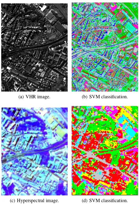
process is applied to both VHR MS and HS image, as depicted in Figure1, which presents VHR MS and HS images and their corresponding classifications (in grey level). It must here be un-derline that in our experiments, VHR MS images were sometimes replaced by panchromatic ones so as to have a more challenging problem.
All SVM classifications considered in this article were obtained using sets of 100 randomly selected pixels for each class within the ground truth data (see Section3.1for more details).
2.2 Basic model
In this section, we present the basic model for MS and HS im-age classification fusion using posterior class probabilities. It is
(a) VHR image. (b) SVM classification.
(c) Hyperspectral image. (d) SVM classification.
Figure 1: Inputs of our method. Two SVM classifications of one multispectral and one hyperspectral image. The label maps are accompanied with posterior class probabilities.
based upon the definition of an energy that will further be mini-mized. The energy is composed of two terms: a data attachment termEdataand a regularization termEregul. This kind of
formula-tion is well known in the image processing domain (Kolmogorov and Zabih, 2004) and has been successfully used for different ap-plications. The energy model is a probabilistic graph taking into account the posterior class probabilitiesPM SandPHSfrom MS
imageIM S and HS imageIHS, respectively, as well as the MS
classificationCM S. In order to get probability maps with
identi-cal sizes,IHS was first upsampled to the size ofIM S, meaning
that each pixel of the VHR MS image has a corresponding pixel in the HS image. For a classification mapC, our basic model defines the energyEas:
E(PM S, PHS, CHS, C) =
X
u∈IM S
Edata(C(u)) (1)
+ λ X
u,v∈N
Eregul(C(u), C(v))
where:
Edata(C(u)) =f(PHS(C(u))),
Eregul(C(u) =C(v)) =g(PM S(C(u)), CM S),
Eregul(C(u)6=C(v)) =h(PM S(C(u)), CM S),
λ∈[0,∞[is the tradeoff parameter between both terms andNis the 8 connexity neighborhood.Edatais a function of the
probabil-ity mapPHSsinceIHS is the data containing the most
discrimi-native information for classification. IfPHS(u)is high, the pixel
Eregulmodels the relationship between a pixel and its neighbors.
The more a pixeluand its neighborsv ∈ Ncorrespond to the desired model, the smallerEregulThe full modelE(C)expresses
how the classification fits to the probability mapPHS and how
neighboring pixels follow the model defined forEregul.
2.2.1 Data term: Edatais the data attachment term and is
de-fined by a functionfsuch as:
f(x) = 1−x, with x∈[0,1].
The functionf ensures that if the probability for a pixeluto belong to the classC(u)is close to1,Edatawill be close to 0 and
will not impact the total energyE. Conversely, if the pixeluis not likely to belong to classC(u),PHS(C(u))will be close to 0
and the data attachment term will be close to its maximum for a pixel, i.e.,1.
2.2.2 Regularization term: The regularization termEregul
de-fines the interaction between a given pixel and its neighbors. For a pixeluand its neighbors inN(the 8 connexity neighborhood), four cases have to be considered regarding the valuesC(u),C(v) andCM S. The four cases considered are the next ones:
Eregul(C(u) =C(v) =CM S(u)) = 0,
Eregul(C(u) =C(v)6=CM S(u)) =PM S(CM S(u))β,
Eregul(C(u) =CM S(u)6=C(v)) = 1−PM S(CM S(u))β,
Eregul(C(v)6=C(u)6=CM S(u)) = 1.
Hence, the regularization term has two functions. The first one is tailored to smooth the results by favoring neighboring pixels to belong to a same class, i.e., whenC(u) =C(v). It is the basic idea of the Potts model (Schindler, 2012) where regularization term is simply defined by:
Eregul(C(u) =C(v)) = 0,
Eregul(C(v)6=C(u)) = 1.
The second role of the regularization termEregulis to take into
account the classificationCM Sof the VHR MS image and, more
specifically, the probabilityPHR(CM S(u))associated to the most
probable classCM S(u). Thus, if a pixeluand one of its neighbor
vare assigned to a same classCand if it also corresponds to the most probable classCM S(u)given by the SVM in the MS image
(i.e., ifC(u) = C(v) = CM S(u)), the regularization term is
null. Indeed, in this case, it is the ”ideal” configuration where the smoothing criterion is satisfied and classificationC(u)matches with the classCM S(u).
IfC(u) = C(v) 6= CM S(u), the smoothing criterion is
satis-fied but the classC(u) does not match with the most probable MS classCM S. In this case, the regularization term is a
func-tion ofPHR(CM S(u)). IfPHR(CM S(u))is high,Eregulis also
high since the likelihood of pixeluto belong to classCM S(u)is
strong.
In the third case,C(u) = CM S(u) 6= C(v), the classification
C(u)matches with the classCM S(u)but the smoothing
crite-rion is not satisfied. IfPM S(CM S(u))is close to1, which means
that SVM on MS image is confident for pixeluto belong to class CM S, thenEregul is small and the configuration is favored.
In-versely, ifPM S(CM S(u))is close to0,Eregulwill be high (close
to1) and the configuration is more prone to be dismissed. The last case is the case where the classC(u)does not match CM S(u)while the smoothing criterion is not satisfied. It is the
worst case, whereC(v)6= C(u) 6=CM S(u). In this case, the
regularization term is set to its maximum value, i.e.,1.
The parameterβ ∈ [0,∞[is a tradeoff parameter between the smoothing criterion and the importance ofCM Sin the model. If
βis high, the smoothing criterion is predominant and the model
comes close to a Potts model. On the opposite, ifβis low, the model will tend to follow the classification given by CM S. A
property that will be used further for parameter selection is that whenβ→ ∞, the proposed model becomes a Potts model.
2.2.3 Energy minimization: The minimization of the energy is performed using a quadratic pseudo-boolean optimization me-thod (QPBO)1. This is a classical graph-cut method that builds a probabilistic graph where each pixel is a node. The minimiza-tion is computed by finding the minimal cut (Kolmogorov and Rother, 2007). QPBO performs regul classification, extension to multi-class problem is performed using anα-expansion routine (Kolmogorov and Zabih, 2004).
2.3 Adding contrast information
In this section, the proposed model is extended to a more gen-eral model that integrates an important visual property contained in the MS image, i.e., the contrast. The contrast is extracted from the VHR MS image since it is the data source with the highest spatial resolution. Indeed, the contrast in the VHR MS image helps retrieving the precise borders between classes and thus improves the classification details. Another smoothness so-lution could have been implicit e.g., by integrating larger regions of analysis such as superpixels that can be sharply detected with standard segmentation algorithms of MS images (Achanta et al., 2012).
Following (Rother et al., 2004) for contrast usage,Vi(u, v) =
exp(−(Ii(u)−Ii(v))2
2(Ii(u)−Ii(v))2)is considered, whereIi(u)is the intensity for pixeluin the MS imageIM Sfor dimensioni.Xis the mean
ofXin the image. The functionV(u, v)computing the contrast value is then given by:
V(u, v, ǫ) = 1
rameter that modifies the standard deviation in the exponential terms.
The general model for classification results fusion is now:
E(PM S, PHS, CHS, C) =
The parameterγis a tradeoff parameter between the basic model (led by the MS classification CM S) and the newly integrated
contrast-based terms.
This model integrates the idea that if the contrast between two neighboring pixelsuandvis important, two pixels are less prone to belong to a same class. Hence, for the condition,C(u) = CM S(u)6= C(v), if the valueV(u, v, ǫ)is high, the
regulariz-ing termEregulwill be high and the configuration will more likely
be rejected. Inversely, for the last conditionC(v) 6= C(u) 6=
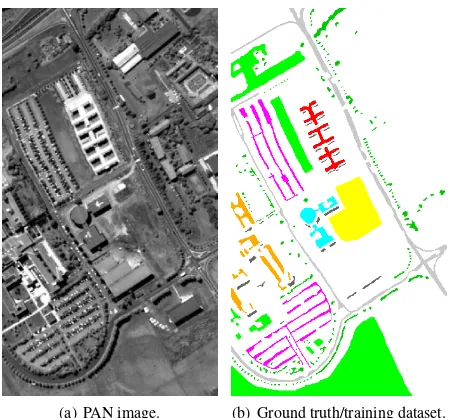
(a) PAN image. (b) Ground truth/training dataset.
Figure 2: Pavia Centre dataset. Classes : Water-Meadows -Trees-Bare soil-Tiles-Bitumen-Asphalt-Self blocking bricks -Shadows.
CM S(u)where the class assigned to pixelsuandvare different,
a high contrast will lead to a small regularizing term.
Ifγ= 0andǫ= 0, the proposed model becomes a Potts model (Schindler, 2012) defined by:
Eregul(C(u) =C(v)) = 0,
Eregul(C(v)6=C(u)) = 1.
This property is used to further address the parameter selection step described in the following section.
2.4 Parameter selection
Parameter selection is always an issue when dealing with ener-gies composed of several terms. The general fusion model de-pends on four parameters, i.e.,λ,β,ǫ, andγ. Parameter selection is performed by cross-validation where a limited part (half of the data here) of the data is used to select the best parameter set (the highest percentage of correct classification). This parameter set is then used to process the rest of the data. The issue here is that choosing the best parameter set among the possible ones might be very costly in computing time.
In order to reduce the computing time of this step, we use the fol-lowing properties of the general model proposed in Section 2.3:
• ifγ= 0andβ→+∞, the general model is a Potts model;
• ifγ= 1andǫ= 0, the general model is a Potts model.
The hypothesis that the valueλmaxmaximizing the classification
result for a Potts model is the same value than the one maximizing the fusion model classification result is formulated here. Hence, λmax is computed using a simple Potts model. Then, withλmax
andγ = 0, βmax is found. Similarly, usingλmax and γ = 1,
the valueǫmaxis computed. Lastly, the tradeoff parameterγmax
maximizing results of the model is chosen in the[0,1]interval. The process can also then be iterated, optimizing parameters in the same order at each iteration.
3. EXPERIMENTS
This section provides first a description of the considered datasets and then presents a discussion on obtained results.
(a) PAN image. (b) Ground truth/training dataset.
Figure 3: Pavia University dataset. Classes :Meadows-Gravel -Trees-Bare soil-Painted metal sheets-Bitumen-Asphalt-Self blocking bricks-Shadows.
3.1 Data
The proposed model was tested on three distinct urban land cover datasets, namelyPavia Centre,Pavia University(Italy) andToulouse Centre(France). Pavia University and Pavia Centre are well known datasets used for years in the hyperspectral community2.
Pavia Centre and Pavia University. Pavia Centre and Univer-sity hyperspectral images have respectively 102 and 103 spectral bands ranging from 430 to 860 nm. Pavia Centre is composed of two images of sizes 228×1096 and 569×1096 pixels. Pavia Uni-versity is a 335×610 pixels image. Both have a ground sample distance (GSD) of 1.3m. Both image ground truths are composed with different sets of 9 classes. The land cover classes associated to Pavia Centre scene are:trees,asphalt,self-blocking bricks, bi-tumen,tiles,shadows,meadows, andbare soil. The set of classes for Pavia University is composed of: meadows, gravel, trees,
painted metal sheets,bare soil,bitumen,self-blocking bricks, shad-ows. For Pavia Centre and Pavia University datasets, a panchro-matic image (PAN) with the initial geometric resolution (1.3 m) was created. In the following, these PAN images were used in-stead of MS images (considering PAN is an extreme case of MS image with only one dimension). This more challenging problem was a way to highlight the properties of the proposed model by using a complex configuration where the geometric precise MS data has very low spectral discriminative properties. The consid-ered HS images were a resampled version at a lower resolution of 7.8 m of the initial HS images. Hence, we have a set of images where the MS image (i.e., here, PAN images) has a 1.3 m geo-metric resolution and HS image has a 7.8 m geogeo-metric resolution. Figures2and3present the PAN/MS image and the ground truth for both Pavia Centre and University datasets.
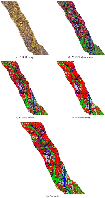
Toulouse. Toulouse Centre dataset was simulated from HS im-ages acquired at a 1.6 m GSD and composed with 405 spectral bands ranging from 400 to 2500 nm (Adeline et al., 2013). MS images composed of 5 bands (in the visible and near infra-red wavelengths) were then simulated at a 1.6 m GSD using the spec-tral configuration of Pliades satellites. HS images were down-sampled to a 8 m GSD. 13 land cover classes were considered:
(a) VHR MS image. (b) Ground truth/training dataset.
Figure 4: Toulouse Centre. Classes : Tiles- Roofing metal 1 -Roofing metal 2-Gravel roof-Slates-Cement-Bare soil -Asphalt- Stone pavement bricks- Water-Meadows- Trees -Shadows.
water,high vegetation(trees) andlow vegetation(bush),asphalt,
tiles,bare soil,metal roof 1 and 2,gravel roof,train track, pave-ment,cement,slates. Figure4shows the MS image of Toulouse Centre dataset and the corresponding annoted ground truth.
3.2 Results
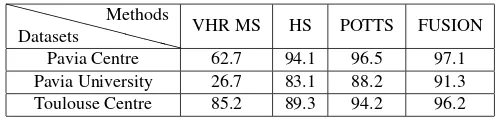
Results obtained on the three datasets are now presented. Fig-ure6shows a table containing the classification results obtained with several variants of the proposed energy. The results shown here were obtained using a cross-validation technique where half of the data was used for parameter selection and the rest is the testing data. Parameter selection for those results followed the method described in Section 2.4. The columns VHR MS and HS correspond to a simple SVM classification applied to the VHR MS (or PAN) and HS data, without any fusion step. These are the input of the basic and general fusion algorithms described in the previous sections. In this figure, the results obtained using a Potts model and the general model proposed in Section 2.3 (FUSION column) are also presented.
The obtained results show the contribution of the fusion of VHR MS and HS images for urban land cover processing. Hence, on the three datasets, classification results were highly increased between SVM classifications on HS/VHR MS data and classi-fication using the proposed fusion model. Moreover, compari-son with a simple Potts model shows that the fusion models pre-sented in this article not only perform smoothing as designed but also correctly use the probability maps to retrieve details avail-able from the VHR MS image (while keeping to some extent the good classification properties of the HS data).
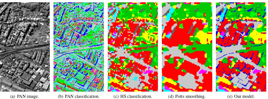
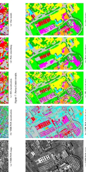
One should note the ground truth corresponds to limited parts of the areas. Thus, even if the classification results are better, quali-tative assessment through visual evaluation on all images remains necessary. This is illustrated in Figure5that shows results of the classification on a restricted area (for visual convenience). The difference on the details of the general shape between the results of the Potts model and the fusion models results is obvious. In-deed, we can distinguish the shape of buildings and roads while it was not possible with the best Potts results. Hence, more than the classification results, the method visually efficiently gets the best of the MS and HS information, providing an efficient classifica-tion (from HS data) while retrieving details provided by the high-est geometric resolution available (from VHR MS data). These properties of the proposed models are observable on Figures7,8
and9. However, it can also be noted that the proposed model is too much focused on MS classification, resulting sometimes in error propagation (e.g.,shadowsare classified aswaterin Fig-ure 5).
During testing, the hypothesis tailored for parameter selection ❳
VHR MS HS POTTS FUSION
Pavia Centre 62.7 94.1 96.5 97.1
Pavia University 26.7 83.1 88.2 91.3
Toulouse Centre 85.2 89.3 94.2 96.2
Figure 6: Classification results (in %).
proved to be empirically efficient. Indeed, we computed the clas-sification results using much more exhaustive sets of parame-ters. We found out that the best classification results were very close from the ones obtained using the procedure described in Section 2.4. Hence the considered hypothesis seems to be valid while significantly reducing the computation costs for parame-ter selection. For example, if the choice is carried out among Nǫ = Nλ = Nβ = Nγ = 100values for the parameter set
{ǫ, λ, β, γ},108 classification processes need to be computed. Such a procedure enables to reduce hugely the computation time for the parameter selection step. Parametersǫ,λ,βand γare selected within grids of sizesNǫ=Nλ=Nβ =Nγ= 100, the
number of classifications to be computed falls from108to400, which is still quite important
4. CONCLUSION
In this paper, we presented a method for fusion of VHR multi-spectral (MS) and hypermulti-spectral (HS) data in urban areas at the decision level. The idea was to combine the best of those two types of data, i.e., the high spatial resolution of MS images and the discriminative properties of the HS images. The proposed fusion model relied on posterior class probabilities, available for most of existing classification techniques. Here, a SVM method was adopted. The probabilities were integrated through an energy minimization process, enabling to improve classification results of a single source and to retrieve details observable in the VHR MS data while keeping the good classification properties obtained with the HS data. The model is generic and intends to be applied to other configuration involving VHR image and richer remote sensing data.
The perspectives are threefold. First, to some extent, the energy should be modified to less rely on posterior class probabilities in order to better manage initial misclassifications or spatial incon-sistencies. Secondly, we will extend our model to a larger set of images (instead of only two here) of various spectral dimensions and geometric resolutions. The idea is to be able to process and fusion any information of a given scene to get the best classifi-cation at the most precise spatial resolution available. This can be performed using a multi-layer process where each layer is the model described in this paper for fusion of two images. Another final interesting perspective is to process MS/HS images acquired at different epochs. This opens the field for change detection in urban areas, and will require more advanced knowledge fusion model.
ACKNOWLEDGMENTS
This work was supported by the French National Research Agency (ANR) through the HYEP project on Hyperspectral imagery for Environmental urban Planning (ANR-14-CE22-0016).
BIBLIOGRAPHY
(a) PAN image. (b) PAN classification. (c) HS classification. (d) Potts smoothing. (e) Our model.
Figure 5: Results on a part of Pavia Centre dataset.
Adeline, K., Le Bris A., Coubard, F., Briottet, X., Paparoditis, N., Viallefont, F., Rivire, N., Papelard, J.-P., David, N., D´eliot, P., Duffaut, J., Poutier, L., Foucher, P.-Y., Achard, V., Souchon, J.-P., Thom, C., Airault, S. and Maillet, G., 2013. Description de la campagne a´eroport´ee UMBRA : ´etude de l’impact anthropique sur les ´ecosyst`emes urbains et naturels avec des images THR mul-tispectrales et hyperspectrales.Revue Franc¸aise de Photogramm´e-trie et de T´el´ed´etection, 202, pp.79–92.
Aitkenhead, M. and Aalders, I., 2011. Automating land cover mapping of Scotland using expert system and knowledge integra-tion methods.Remote Sensing of Environment, 115(5), pp.1285– 1295.
Benediktsson, J.A. and Kanellopoulos, I., 1999. Decision fusion methods in classification of multisource and hyperdimensional data. IEEE Trans. on Geoscience and Remote Sensing, 37(3), pp.1367–1377.
Breiman, L., 2001. Random Forests. Machine Learning, 45(1), pp.5–32.
Carper, W.J., Lillesand, T.M. and Kiefer, R.W., 1990. The use of Intensity-Hue-Saturation transform for merging SPOT panchro-matic and multispectral Image Data.Photogrammetric Engineer-ing & Remote SensEngineer-ing, 56 (4), pp.459–467.
Ceamanos, X., Waske, B., Benediktsson, J.A., Chanussot, J., Fau-vel, M. and Sveinsson, J.R., 2010. A classifier ensemble based on fusion of Support Vector Machines for classifying hyperspec-tral data. International Journal of Image and Data Fusion, 1(4), pp.293–307.
Chavez, S., Stuart, J., Sides, C. and Anderson, J.A., 1991. Com-parison of three different methods to merge multiresolution, mul-tispectral data Landsat TM and SPOT panchromatic. Photogram-metric Engineering & Remote Sensing, 57(3), pp.259–303.
Fauvel, M., Chanussot, J. and Benediktsson, J.A., 2006. De-cision fusion for the classification of urban remote sensing im-ages. IEEE Trans. on Geoscience and Remote Sensing, 44(10), pp.2828–2838.
Gamba, P., 2014. Image and data fusion in remote sensing of ur-ban areas: status issues and research trends. International Jour-nal of Image and Data Fusion, 5(1), pp.2–12.
Huang, X. and Zhang, L., 2012. A multilevel decision fusion approach for urban mapping using very high-resolution multi-hyper-spectral imagery.International Journal of Remote Sensing, 33(11), pp.3354–3372.
Joshi, N. et al., 2016. A review of the application of optical and radar remote sensing data fusion to land use mapping and moni-toring.Remote Sensing, 8(1):70.
Khatami, R., Mountrakis, G. and Stehman, S., 2016. A meta-analysis of remote sensing research on supervised pixel-based land-cover image classification processes: general guidelines for practitioners and future research. Remote Sensing of Environ-ment, 177, pp.89–100.
Kolmogorov, V. and Zabih, R., 2004. What energy functions can be minimized via Graph Cuts?IEEE Trans. on Pattern Analysis and Machine Intelligence, 26(2), pp.65–81.
Kolmogorov, V. and Rother, C., 2007. Minimizing non-submodular functions with Graph Cuts - a review. IEEE Trans. on Pattern Analysis and Machine Intelligence,29(7), pp.1274–1279.
Loncan, L., Almeida, L. B., Bioucas-Dias, J. M., Liao, W., Briot-tet, X., Chanussot, J, Dobigeon, N., Fabre, S., Liao, W., Liccia-rdi, G., Simoes, M., Tourneret, J.-Y., Veganzones, M., Vivone, G., Wei, Q. and Yokoya, N., 2015. Hyperspectral pansharpening: a review.IEEE Geoscience and Remote Sensing Magazine, 3(3), 27-46.
Platt, J., 2000. Probabilistic outputs for Support Vector Machines and comparison to regularized likelihood methods. In: A. Smola, P. Bartlett, B. Sch¨olkopf, and D. Schuurmans (eds.): Advances in Large Margin Classifiers.MIT Press. Cambridge, MA, USA.
Rother, C., Kolmogorov, V. and Blake, A., 2004. ”Grabcut” -Interactive foreground extraction using iterated graph cuts.ACM Trans. on Graphics, 23(3), pp.309–314.
Sch¨olkopf, B. and Smola, A.J., 2002. Learning with kernels: Support Vector Machines, regularization, optimization and be-yond.MIT press, Cambridge, MA, USA.
Schindler, K., 2012. An overview and comparison of smooth labeling methods for land-cover classification. IEEE Trans. on Geoscience and Remote Sensing, 50(11), pp.4534–4545.
Szeliski, R., 2010. Computer Vision: algorithms and applica-tions.Springer-Verlag, London, UK.
Shafer, G., 1976. A mathematical theory of evidence. Princeton University Press, Princeton, NJ, USA.
(a)
VHR
P
AN
image.
(b)
VHR
P
AN
classificat
ion.
(c)
HS
classificat
ion.
(d)
Potts
smoothing.
(e)
Our
m
odel.
Figure
7:
P
avia
Centre
results.
(a)
VHR
P
AN
image.
(b)
VHR
P
AN
classification.
(c)
HS
classification.
(d)
P
otts
smoothing.
(e)
Our
model
.
Figure
8:
P
avia
Uni
v
ersity
(a) VHR MS image. (b) VHR MS classification.
(c) HS classification. (d) Potts smoothing.
(e) Our model.