ACCURATE OPTICAL TARGET POSE DETERMINATION
FOR APPLICATIONS IN AERIAL PHOTOGRAMMETRY
D. A. Cucci
´
Ecole Polytechnique F´ed´erale de Lausanne (EPFL), Switzerland - (davide.cucci)@epfl.ch
Commission III, WG III/3
KEY WORDS:Optical Targets, Tragets Orientation, Image Processing Algorithms, Navigation, Geometry
ABSTRACT:
We propose a new design for an optical coded target based on concentric circles and a position and orientation determination algorithm optimized for high distances compared to the target size. If two ellipses are fitted on the edge pixels corresponding to the outer and inner circles, quasi-analytical methods are known to obtain the coordinates of the projection of the circles center. We show the limits of these methods for quasi-frontal target orientations and in presence of noise and we propose an iterative refinement algorithm based on a geometric invariant. Next, we introduce a closed form, computationally inexpensive, solution to obtain the target position and orientation given the projected circle center and the parameters of the outer circle projection. The viability of the approach is demonstrated based on aerial pictures taken by an UAV from elevations between10to100m. We obtain a distance RMS below0.25% under50m and below1% under100m with a target size of90cm, part of which is a deterministic bias introduced by image exposure.
1 INTRODUCTION
Optical coded targets consist in distinctive visual patterns de-signed to be automatically detected and measured in camera im-ages. A number of different designs have been proposed in the literature, all of them having the following properties: i) low or no similarity with common environmental features, ii) robust dis-ambiguation between multiple instances, usually by means of sig-nals encoded in the marker, iii) cheap and robust detection algo-rithm. Some examples are shown in Figure 1. Particular atten-tion is currently being given to square coded markers due to the availability of powerful and ready to use augmented reality li-braries, such as ARToolKit (Wagner et al., 2008), AprilTags (Ol-son, 2011), and arUco (Garrido-Jurado et al., 2014). Even tough visual targets are well studied in the literature, this field is still fertile for research in specific applications such as camera cali-bration, photogrammetry, robotics, augmented reality and in ma-chine vision techniques in general.
In this work we propose a design for an optical target and a novel detection and measuring algorithm for which the requirements are driven by a specific application within the mapKITE project1.
In this project, a new mapping paradigm is introduced in which a terrestrial-aerial tandem, composed by a human driven terrain ve-hicle (TV), and an autonomous micro aerial veve-hicle (UAV), per-forms the surveys, augmenting terrestrial laser range-finder data with a aerial photography (Molina et al., 2015).
The UAV is required to autonomously follow the terrain vehicle during mapping. Normally, the TV transmits its position to the UAV via a radio link. However, the connection between the two vehicles may be lost or the position of the TV might become tem-porarily unavailable, e.g., because of GPS outages. Thus, optical guidance is also considered. In this context, the tracking algo-rithm must primarily exhibit a very low percentage of false posi-tive tracks, which could catastrophically deceive guidance strate-gies, and secondarily, a low percentage of false negative tracks, to allow for smooth following and reduced probability of losing the TV. The optical target is also beneficial in post-processing:
1
See acknowledgments.
(a) Schneider, 1991 (b) Ahn, 2001 (c) arUco, 2014
Figure 1: Examples of fiducial targets commonly employed in robotics and photogrammetry applications.
if the accuracy of the target center and distance measurements is high enough, the TV position can be employed to build kine-maticground control point (KGCP) to be used in assisted aerial triangulation (AAT) (Molina et al., 2016).
Our solution, depicted in Figure 2, is a multi-scale design that makes use of a code for robust detection and multiple concentric circles for the determination of the target center projection and of the target orientation with respect to the camera. We prefer to use large circles instead of relying on corner features, as it is com-mon in square coded markers, e.g. the one in Figure 1(c), since circle projections, ellipses on the image plane, are cheaply and robustly detected and their defining parameters can be accurately determined by means of closed form least-squares curve fitting. Furthermore, while the information on the position of a corner tend to concentrate in one single pixel as the distance increases, the ellipse center and dimensions are embodied in the coordinates of tents to hundreds of edge pixels, even from high distance.
Figure 2: The optical target used in this work. The target code is obtained sampling on the red dashed line.
2 OPTICAL TARGET DESIGN AND DETECTION
The optical target employed in this work is depicted in Figure 2. Its main features are: i) two large circles replace corners or point features for relative position and orientation determination, ii) the position of the white dots in the black ring encode a signal that is employed for robust detection and 2D orientation determina-tion, iii) multiple (one, in this case) replica can be superimposed with different scales and distinguished thanks to a different target code. This fractal design is necessary to allow at least one target to be fully visible from low distances and it has been considered for automated landing based on optical guidance.
In the following we summarize the main image processing steps employed in the target detection.
2.1 Contours Detection
The first step involves isolating edges, i.e., pixels with high inten-sity gradient. We employ the Canny detector and then we group positive pixels to form closed contours as in (Suzuki et al., 1985).
2.2 Circles Detection
In the general case, the circular target will appear as an ellipse once projected on the image plane. However, in our application the nominal distance from the target and the limitations on the allowed UAV orientations limit the perspective deformation, so that we can select candidate targets searching for approximately circular contours. To do so we use a computationally inexpensive, yet very effective, test: for each contour, we compute its center Diaveraging the coordinates of the edge pixels, then we compute
the meanµiand the standard deviationσiof the distance between
each edge pixel andDi. We accept a contour if: i)µi > µM IN
and ii)σi< kµi, whereµM INandkare two parameters of the
algorithm. Note that if thei-th contour is exactly a circle,σiis
zero, while moderate values ofkallow ellipsoidal contours to be also accepted. Finally, we form clusters of concentric circles with similar center coordinates and for each cluster we mark the circle with largest radius as the cluster representative.
2.3 Code Test and Target Heading Determination
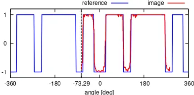
We test the inside of each cluster representative for the presence of the target code. We obtain a one dimensional signal sampling the image along the red line in Figure 2, which is defined accord-ing to the measured center and radius of the cluster representative. This line intersect the white dots in the black outer ring at specific
-1 0
-73.29
-360 -180 0 180 360
angle [deg]
Figure 3: Target signal test and orientation determination.
angles and the black/white alternation forms a periodic signal, as a function of the angle. Different codes can be obtained changing the position of the dots, allowing for multiple target tracking and for target scale resolution in case multiple replicas are detected. The signal obtained sampling the image is matched with the ref-erence signal maximizing their normalized cross-correlation (see Figure 3). The cluster representative for which the normalized cross correlation is maximum, and exceeding a minimum thresh-old, is selected as the final target candidate.
The target 2D orientation on the image plane is also measured: it corresponds to the lag between reference and image signals for which the normalized cross correlation is maximum. While encoded signals are widely employed in optical target detection to reject false matches and to allow for multiple target tracking, the authors are not aware of other target designs that employ signals to measure 2D orientation.
The target 2D orientation is a desirable output at early stages of the tracking pipeline as a naive optical-based TV following could be implemented employing only the information extracted so far, e.g. target position and 2D orientation on the image plane, if an external elevation control strategy is available.
2.4 Sub-pixel Edge Detection and Ellipse Fitting
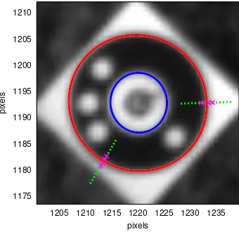
Once the correct outer circle has been identified, we search in the corresponding circles cluster for the inner one. Next, we fit two preliminary ellipses on the contours corresponding to the two concentric circles, marked in green in Figure 2. This involves finding the parametersQ′ of the ellipse equationxTQ′x = 0,
withQ′being a symmetric3×3matrix with eigenvaluesλ 1, λ2>
0andλ3<0, such that it best fits the coordinates of the edge
pix-els. This problem can be solved in least-square sense and a closed form solution exists, e.g., see (Fitzgibbon et al., 1996).
The determined ellipses are then refined with sub-pixel edge de-tection. We determine4√a2+b2
points on the ellipse, where a andbare the ellipse major and minor axis. The number of points is a lower bound for the ellipse perimeter. For each of those points, we sample the original image at four locations on a line orthogonal to the ellipse contour (see Figure 4) and we fit a 3-rd order polynomial on the obtained intensities. The inflection point of this polynomial gives the position of the sub-pixel edge point. Finally, we correct the sub-pixel edge points coordinates for lens radial and tangential distortion and we repeat the ellipse curve fitting steps employing the set of refined edge points.
At this stage we have fitted on the image two ellipses, correspond-ing to the projection of the two concentric circle of the target, and we have obtained the related parametersQ′
oandQ′i. From now
on, we will not perform any further measurement on the image.
3 TARGET POSE DETERMINATION
1175 1180 1185 1190 1195 1200 1205 1210
1205 1210 1215 1220 1225 1230 1235
pixels
pixels
Figure 4: Sub-pixel edge detection and ellipse fitting. The outer ellipse major and minor axis are respectively13.320and12.876 pixel long, while the contour is composed of150edge pixels. The image correspond to real-world data and it is taken from a distance of98.6m.
To this end, let us assume for the moment that we know very precisely the position of the projection of the concentric circles center. We will discuss how this can be obtained in Section 4.
In Figure 5 we have sketched the target pose determination prob-lem:Ois the optical center of the camera,Cis the center of the target, segmentABis the target diameter that is coplanar with the yaxis of the camera frame. The sketch is a projection of the scene on theyzplane. As we have assumed, we know very precisely the position of the projected circle center in the image plane, C′. Moreover, we have estimated the parameters of the
ellipseQ′
o, being the projection on the image plane of the
tar-get outer circle. We determine analytically the intersection ofQ′ o
with a line troughC′ and parallel to theyaxis of the camera
frame, obtaining the pointsA′andB′in the image plane. This
points correspond to the projection ofAandB.
Three viewing rays, directions in camera frame, correspond to the three pointsA′,B′, andC′ and they can be determined by
pre-multiplying image point coordinates with the inverse of the intrinsic camera calibration matrix, and then normalizing, e.g.:
~vA=
K−1
A′
||K−1A′
||. (1)
Note that in general~vA,~vBand~vCdo not belong to theyzplane,
as it might appear from the drawing in Figure 5, where we have drawn their projection on that plane.
Next, the anglesθ1andθ2can be determined from thedot
prod-uct of the viewing rays:
θ1= cos− 1
(~vA·~vC), (2)
θ2= cos− 1
(~vB·~vC). (3)
We are now ready to determine the length ofOC, which is the tar-get distance. This problem can be seen as a two-dimensional in-stance of the well known Perspective-3-Points (P3P) problem (Fis-chler and Bolles, 1981, Wu and Hu, 2006). A closed form solu-tion can be obtained by applying the cosine theorem to the
trian-Figure 5: Target pose determination problem, projection on the yzplane of the camera frame. Ois the camera optical center, Cis the target center and the segmentABis the target diameter which is coplanar to theyaxis. ClearlyAC=BC=r.
glesAOC,COBandAOB, i.e.,
r2
=OA2+OC2−2OA OCcos(θ1)
r2
=OB2+OC2−2OB OCcos(θ2)
(2r)2
=OA2+OB2−2OA OBcos(θ1+θ2)
, (4)
whereris the target radius and the length of the segmentsAC andBC. Solving inOCyields:
OC=
√
2rsin(θ1+θ2) p
3−2 cos(2θ1)−2 cos(2θ2) + cos(2(θ1+θ2))
,
(5)
We can also determine the angleφ, which is the misalignment of the considered target diameterABwith respect to theyaxis of the camera frame: first we determine the anglesγ1 andβ2,
applying the sine theorem to the trianglesAOCandCOB:
γ1= sin− 1
OC
r sin(θ1)
, (6)
β2= sin− 1
OC r sin(θ2)
. (7)
Each equation gives two solutions, sincesin(α) = sin(π−α), yet only one couple(γ1, β2)satisfies
θ1+γ1+ (π−γ2) =θ2+γ2+β2=π. (8)
We can now determineOB, the vector~vOBandφ:
OB=rsin (π−β2−θ2) sinθ2
, (9)
~vOB=OB~vB−OC~vC, (10)
φ= tan−1
(~vOB,y, ~vOB,z). (11)
The angleφis the roll angle of the relative orientation of the target with respect to the camera. Indeed this angle is formed by thez axis of the camera frame and the target diameterAB, that has been chosen to lie in theyzplane. To determine the pitch angle θ, the procedure just discussed is repeated, this time intersecting the ellipseQ′
o with a line troughC′ and parallel to thexaxis,
thus obtaining the projection of a diameter lying in thexzplane.
4 PROJECTION OF THE CIRCLE CENTER
It remains to discuss how the coordinates of the projection ofC can be determined. Note that this point isnotthe center of either Q′
oorQ′i, as it can be seen remembering that perspective
15.2
o)as a function ofγfor five random points
˜
C′in the neighborhood ofC′. The ellipseQ′
ois the outer circle
projection of a target placed a true distance of15.56m.
not to employ corner features to locateC′since these would not
be sharp or visible from high distance, as it is clear from Figure 4.
One known solution to determine the image coordinates ofC′is
to employ two concentric circles, such asQoandQi. Once the
parameters of two ellipses have been fitted to the pixels compos-ing the correspondcompos-ing contours, a quasi-analytical solution exists forC′: letλbe the repeated eigenvalue ofQ′
i is the homogeneous coordinate of the
projected circle center. For the proof see (Kim et al., 2005).
The afore-discussed result holds only if theestimatedellipsesQ′ o
andQ′
iare projections of concentric circles. In other words, in
order forQ′
oandQ′ito be the projections of two concentric
cir-cles, certain constraints must be satisfied by their parameters, see again (Kim et al., 2005). So constrained estimation should be employed to jointly fitQ′
oandQ′ion the edge pixels. If this is
not the case, as in (Yang et al., 2014) and in this work, i.e, the two parameter sets are estimated independently, geometric con-straints between the two ellipses may not hold exactly. In prac-tical applications this causesQ′
iQ′− 1
o not to have any repeated
eigenvalue, but two very similar ones, and the non-zero rows is Q′−1
o −λQ′−
1
i being slightly different, whereas they should be
equal. This gives up to six candidates forC′. As we will show in
the following, in general these solutions are not accurate enough for being employed in the method discussed in Section 3.
We discuss here a technique to improve the estimate ofC′
ob-tained with the Kim’s method. We first define a functiondthat, for a given ellipseQ′, estimatesOCas a function of the
coordi-nates of the projected circle center, as in Section 3, yet, to obtain A′andB′, we intersectQ′
owith an arbitrary line troughC′, and
parametrized with an angleγ. Thus we have:
OC=d(C′, γ, Q′),
(12)
whereγis the angle formed by the line used to intersectQ′and
thexaxis of the image plane. Note that in Section 3 we used a vertical line, i.e.,γ=π/2to determineφ, and an horizontal one, i.e.,γ= 0, to determineθ. We would like to stress the fact that the functiond(·)is analytical.
Suppose now that we have applied the Kim’s method based on the repeated eigenvalue ofQ′
iQ′− 1
o and we have obtained an initial
guess for the projection of the circle center,Cˆ′. As anticipated,
this estimate is problematic in practical cases and it is not accurate enough to be employed for computingOC. To understand why, consider the following reasoning: ifCˆ′is the true projection of
the circle center, the functiond( ˆC′, γ, Q′)must return the same
value for every choice of the angleγ. In fact, ifCˆ′is the projected
circle center, whatever line passing throughCˆ′will intersect the
116
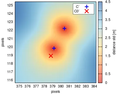
minor axis 91.02 and 76.46 px, angle −113.81◦ and center
(379.43,120.55). Marked points are the two candidates for the projected circle centerC′ and the solution obtained employing
the method in (Kim et al., 2005).
ellipseQ′ in two points being the projection of one diameter of
the circle and thus enabling the reasoning discussed in Section 3. Instead, ifCˆ′is not the projected circle center, the segmentAB
is not a diameter and in generalAC6=BC6=r. Thus, even for subtle deviations ofCˆ′from its true coordinates,d( ˆC′, γ, Q′)
re-turns different distances for different values ofγ. As an example, we have chosen an ellipseQ′
ocorresponding to a target placed at
15.56m and we have plottedd( ˜C′, γ, Q′
o)for five random points
˜
C′sampled in the close neighborhood of the true projected circle
center (σ= 0.1pixels). See Figure 6. Variations ind( ˜C′, γ, Q′ o)
of the order of0.5m are obtained.
The aforesaid reasoning gives us a very sensitive geometric in-variant that we can employ to improve our initial guess forC′:
D( ˜C) := stdγ
Namely, for a given ellipse Q′
o we search for the pointC˜′ for
which the dispersion of the values ofd( ˜C′, γ, Q′
o)is minimum.
As we know, there exist at least one pointC˜′for whichD( ˜C′)is
identically zero, being the true projection of the circle center.
The landscape of the functionD( ˜C′)is depicted in Figure 7 for
the ellipse Q′
o employed in the previous example. It is
imme-diately evident that in this case there are two global minima for D( ˜C′). To see why, consider again Figure 5 and take the
sym-metry ofAandBaround the bisector of the angle∠AOB: the same projectionsA′ andB′ are obtained but the orientation of
the target and the projection of the circle centerC′are different.
It is not possible to discriminate between the two orientations, or decide for one of the two attractors in Figure 7 employing only the projection of one circle contour. However, for what concerns target distance estimation, the existence of two projected circle center candidates is not an issue since the same distance is as-sociated to both points (swapθ1 andθ2in Equation 5). A very
0 20 40 60 80 100
10 20 30 40 50 60 70 80 90 100 0 40 80 120 160 200
detection probability [%]
marker size [pixel]
true distance [m]
Figure 8: Estimate of the detection probability as a function of the true distance from the camera.
To solve the minimization problem in Equation 14 we employ a gradient descent search strategy with adaptive learning rate and we initialize the search with the solution obtained with Kim’s method. The function to be optimized is reasonably regular and the initial guess is already close to one global optimum. Note that the initial guess is computed employing both the inner and the outer ellipses, in which case the solution is unique. Thus we conjecture that in most of the cases the initial guess lies in the attractor basin of the true projected circle center.
In this section we have presented very sensitive method to deter-mine the coordinates of the projected circle center, which enables the pose determination method in Section 3. We would like to stress the fact that in the presented algorithm the only quanti-ties that are measured on the image are the parameters of the el-lipsesQ′
oandQ′i. All the other quantities are analytical or
quasi-analytical functions of these parameters. Indeed, fromQ′ oandQ′i
we derive an initial guess forC′with the Kim’s method. Then,
onlyQ′
o is employed in the numerical minimization ofD( ˜C′),
yieldingC′. The coordinates ofC′are finally plugged in the
ex-pressions in Section 3 to determineOC,φandθ. So the accuracy and precision of the pose estimation greatly depend on the pro-cedure employed to measureQ′
o andQ′oin the image, from the
edge detection to the curve fitting.
5 EXPERIMENTAL EVALUATION
In this section we evaluate the target detection algorithm based on synthetic and real-world images. To this end, we flew with a cus-tom octo-copter over the optical target and we acquired pictures at relative elevations between10and100m.
We employed a Ximea MQ042MG4Mpx camera equipped with 16mm lenses, pointing down, which gives us a GSD of3.5cm and a field of view of70m at100m elevation. The radius of the target outer circle is0.9m. We determined the intrinsic camera calibration matrix and lens distortion coefficients during a sep-arate flight over a dedicated calibration field. To obtain ground truth positions for the camera optical center and for the marker center we oriented the collected frames by means of AAT.
The detection algorithm proved to be very robust: the target was successfully detected in1807frames out of2134(84.7%). An estimate of the probability that the target is detected as a function of the true distance is shown in Figure 8. Based on these em-pirical results we argue that the detection is reliable if the target diameter size in the image is bigger than40pixels, which trans-lates, given the considered choice of camera and lenses, to a flight elevation lower than 80m. Moreover, a deceiving target, i.e., a target with the same geometry but different code, was placed nearby. The deceiving target was selected in only5images, con-firming the viability of the approach in multi-target applications.
-2.5 -2 -1.5 -1 -0.5 0 0.5 1
10 20 30 40 50 60 70 80 90 100
error [m]
true distance [m]
µ
3σ
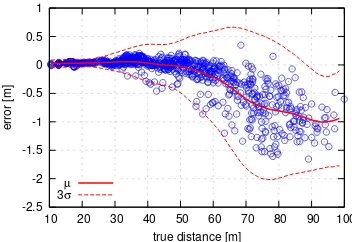
Figure 9: Error in distance measurement as a function of the true distance. We have also plotted a moving average and standard deviations computed with window size10m.
−22cm −15cm 38.41m +2cm +4cm
−72cm −16cm 97.07m +20cm +68cm Figure 10: Effect of different exposures on the estimated dis-tance for two frames at nominal disdis-tance of38.41m and97.07 m (darker on the left, brighter on the right, original in the center).
In Figure 9 we have plotted the difference between the reference distance, i.e.,OCin Figure 5, and the one computed with the de-scribed tracking algorithm. The red curves are windowed average and standard deviations. It is possible to see that the algorithm yields unbiased and very precise distance measurements up to50 m while at higher elevation the distance measurement appears to be biased by some deterministic effect, even thought mean error remains below1% of the distance. We don’t experience a com-parable effect in synthetic data.
One possible explanation is the following: sharp edges becomes gradients in camera images due to lens point spread function and blurring. The sub-pixel edge detection presented in Section 2.4 aims at recovering the precise edge location from these gradi-ents. However, different camera exposures yield different gra-dients, making the ellipses appear slightly bigger or smaller and thus giving different distance estimation. An example is given in Figure 10, where we show that if we artificially change the ex-posure we obtain different distance estimates, depending on the elevation. This can motivate the deterministic bias visible in Fig-ure 9. In order to increase the distance accuracy we have to either precisely control the exposure of each frame or have a sub-pixel edge detector that is invariant with respect to exposure.
Other possible reasons are: i) the geometry of the photogram-metric problem is rather weak as the flight involved a climb and a descent always pointing the same area. It is possible that the ob-tained reference positions from AAT are not sufficiently accurate. Unfortunately, camera positions uncertainties are not provided by the commercial software used for image orientation; ii) the intrin-sic camera calibration is not constant and can change because of temperature, vibrations and other effects. It is possible that some distortion between reference positions and estimated target dis-tance is due to slight variations in the camera calibration.
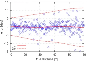
-15 -10 -5 0 5 10
10 20 30 40 50 60
error [deg]
true distance [m] µ
3σ
Figure 11: Error inφmeasurement on synthetic images.
from random camera positions and orientations. It is possible to see that while the estimates are unbiased, the error standard devi-ation is quite high even at low distances. This is expected as the marker distance is10to50times bigger than the marker radius.
6 CONCLUSIONS AND FUTURE WORK
In this work we have introduced a novel optical target design de-veloped with the goal of determining with high accuracy its center and its distance from UAV-based mapping elevations. An experi-mental evaluation based on real-world data has show remarkable accuracy and has shown that further improvements can be ob-tained correcting for the exposure induced bias.
The presented position and orientation determination algorithm works on the estimated parameters of the two ellipses correspond-ing to the outer and inner circles in the marker. These parameters are robustly estimated in least-squares sense from a set of sub-pixel edge points. This step is crucial for the accuracy of the distance and orientation measurements, as no other quantities are measured on the image. One direct way to improve this step is the following: at the present stage, the two ellipses are estimated independently. This does not exploit the fact that they are the projection of two concentric circles. The curve fitting problem can be reformulated so that the constraints existing between the ellipse parameters are kept into account during estimation. More-over, the effects of varying exposure on the edge positions on the image has to be investigated as biases might exist in the employed sub-pixel detection method.
After the two ellipses are determined, the projection of the circle center is estimated numerically minimizing an analytical non lin-ear function of the outer ellipse parameters. Two attractor basins, and thus two candidates for the circle center projection, exist for this function. These two candidates correspond to two pos-sible orientations for the target. The orientation ambiguity can be solved employing the second ellipse. We argue that it should be possible to obtain the coordinates of the two candidates in closed form as a function of the outer ellipse equation only. This would remove the need for the numerical minimization.
After the projected circle center coordinates have been determined, the distance and the orientation of the target are determined an-alytically. A error propagation analysis has to be performed to provide confidence interval for these quantities as a function of the uncertainty on ellipse parameters, which comes from least-squares curve fitting, and as a function of the intrinsic camera calibration parameters.
ACKNOWLEDGEMENTS
This work was partially funded by the European Community Hori-zon 2020 Programme under grant agreement no. 641518 (project
REFERENCES
Fischler, M. A. and Bolles, R. C., 1981. Random sample consen-sus: a paradigm for model fitting with applications to image anal-ysis and automated cartography. Communications of the ACM 24(6), pp. 381–395.
Fitzgibbon, A. W., Fisher, R. B. et al., 1996. A buyer’s guide to conic fitting. DAI Research paper.
Garrido-Jurado, S., Muoz-Salinas, R., Madrid-Cuevas, F. and Marn-Jimnez, M., 2014. Automatic generation and detection of highly reliable fiducial markers under occlusion. Pattern Recog-nition 47(6), pp. 2280 – 2292.
Kim, J.-S., Gurdjos, P. and Kweon, I.-S., 2005. Geometric and algebraic constraints of projected concentric circles and their ap-plications to camera calibration. IEEE Transactions on Pattern Analysis and Machine Intelligence 27(4), pp. 637–642.
Molina, P., Bl´azquez, M., Sastre, J. and Colomina, I., 2015. A method for simultaneous aerial and terrestrial geodata acquisi-tion for corridor mapping. The Internaacquisi-tional Archives of Pho-togrammetry, Remote Sensing and Spatial Information Sciences XL-1/W4, pp. 227–232.
Molina, P., Bl´azquez, M., Sastrea, J. and Colominaa, I., 2016. Precision analysis of point-and-scale photogrammetric measure-ments for corridor mapping: Preliminary results. The Interna-tional Archives of Photogrammetry, Remote Sensing and Spatial Information Sciences XL-3/W4, pp. 85–90.
Olson, E., 2011. AprilTag: A robust and flexible visual fiducial system. In: Proceedings of the IEEE International Conference on Robotics and Automation (ICRA), IEEE, pp. 3400–3407.
Schweighofer, G. and Pinz, A., 2006. Robust pose estimation from a planar target. IEEE Transactions on Pattern Analysis and Machine Intelligence 28(12), pp. 2024–2030.
Suzuki, S. et al., 1985. Topological structural analysis of digitized binary images by border following. Computer Vision, Graphics, and Image Processing 30(1), pp. 32–46.
Tanaka, H., Sumi, Y. and Matsumoto, Y., 2014. A solution to pose ambiguity of visual markers using moir´e patterns. In: Intelligent Robots and Systems (IROS 2014), 2014 IEEE/RSJ International Conference on, IEEE, pp. 3129–3134.
Wagner, D., Reitmayr, G., Mulloni, A., Drummond, T. and Schmalstieg, D., 2008. Pose tracking from natural features on mobile phones. In: Proceedings of the 7th IEEE/ACM Interna-tional Symposium on Mixed and Augmented Reality, IEEE Com-puter Society, pp. 125–134.
Wu, P.-C., Tsai, Y.-H. and Chien, S.-Y., 2014. Stable pose track-ing from a planar target with an analytical motion model in real-time applications. In: Mulreal-timedia Signal Processing (MMSP), 2014 IEEE 16th International Workshop on, IEEE, pp. 1–6.
Wu, Y. and Hu, Z., 2006. Pnp problem revisited. Journal of Mathematical Imaging and Vision 24(1), pp. 131–141.