Long-term simulation of water movement in soils
using mass-conserving procedures
Peter Berg
Department of Environmental Sciences, University of Virginia, Charlottesville, VA 22903, USA
(Received 29 December 1997; revised 3 July 1998; accepted 1 August 1998)
Three implicit numerical procedures for solving Richards’ equation were compared. In some tests non-linear source terms were included. The main focus is on two mass-conserving procedures where the highly non-linear nature of Richards’ equation is overcome by substantially different iterative techniques. In the first procedure (P1), which is well described in the literature, the time step is set back when difficulties in obtaining a convergent solution occur and any source terms are included explicitly. The second procedure (P2), which is presented in this paper, uses a fixed time step and convergence is obtained through a gradually increasing underrelaxation technique. Source terms are included implicitly, and in addition, a linear dependency between source terms and the water potential is included directly in the solution. The third procedure (P3) is based on a standard implicit discretization of Richards’ equation, which does not facilitate mass conservation. All tests showed that mass conservation can be obtained without the added cost of more complicated programming or a longer calculation time. In challenging tests where fluctuating boundary conditions were specified as known fluxes, the total number of iterations needed in P1 to simulate the tests was many orders of magnitude higher than that for P2. In tests including source terms, the more advanced treatment of these in P2 resulted in convergence rates that were significantly higher that for the explicit coupling in P1. The gradually increasing underrelaxation technique and the more advanced treatment of source terms in P2 have proven to be effective approaches, particularly in long-term simulations of water movements in soils where calculation time can be prohibitive. As a secondary benefit, the implementation of P2 is less complicated than P1.q1999 Elsevier Science Ltd. All rights reserved.
Keywords: long-term simulations, Richards’ equation, mass-conserving procedures.
1 INTRODUCTION
Although Richards’ equation18 is only strictly valid for incompressible soils where water flows isothermally in the soil matrix (no macro-pore flow), it is widely used to describe transient water flow in realistic field situations. As outlined by Parlange et al.,16 analytical solutions of Richards’ equation have become more advanced, but numerical techniques must still be applied in order to obtain a general solution when soil inhomogeneities, fluc-tuating boundary conditions, plant uptake, and drainage are taken into account. This has been done in many models such as DAISY,6SOIL/SOILN10,12and RZWQM1where trans-port of water is coupled to plant growth and the transtrans-port of energy and nitrogen in a detailed description of the
soil–plant–atmosphere system. Such models are typically used in long-term studies where many years are simulated repeatedly and often require excessive calculation time. Because of the strong non-linear nature of Richards’ equa-tion, the numerical sub-solution of this equation is com-monly the most challenging part, and many studies have focused on developing more effective and reliable numeri-cal procedures for solving this particular equation.13 As shown by Milly and Eagleson,15 common standard discre-tization techniques give a finite mass balance error that cannot be neglected unless extremely small time steps are used. Thus, it was a major step forward when different mass-conserving schemes were presented in the 1980s that allowed much larger time steps, while still keeping a good discrete approximation of Richards’ equation.15,5,14,2,4,3
q1999 Elsevier Science Ltd Printed in Great Britain. All rights reserved 0309-1708/99/$ - see front matter
PII: S 0 3 0 9 - 1 7 0 8 ( 9 8 ) 0 0 0 3 2 - 3
Issues other than obtaining mass conservation when solving Richards’ equation are clearly important as well; the strong non-linear nature of the Richards’ equation often causes serious problems in the iterative search for a convergent solution. In extreme situations, some schemes simply fail to find a convergent solution. In addition, source terms that are non-linear functions of the soil water potential, which normally are present when dealing with realistic field situations, can have additional negative effects on a procedure’s ability to find a convergent solution. These problems are addressed in the present study where the performance and ease of implementation for three procedures for solving Richards’ equation are compared.
The first procedure (referred to as P1) is based on the popular implicit and mass-conserving iteration scheme by Celia et al.,3,4 and is implemented as described by Ahuja
et al.1The second procedure (P2) is a new procedure, where mass conservation is obtained by applying the approxi-mation of the specific water content suggested indepen-dently by Cooley5 and Milly.14 The third procedure (P3) is based on a standard implicit discretization, and for that reason it does not facilitate mass conservation. The main focus is on the two mass-conserving procedures where the problems arising from the described non-linearities are solved in significantly different ways.
2 THEORY
All three procedures produce solutions of Richards’ equation where a source term has been included:
]v
wherevis the volumetric soil water content,w is the soil water potential, K is the hydraulic conductivity, t is the time, z is the depth below the soil surface, assumed to be positive downward, and S is the source term.
The iteration schemes in the three procedures are listed below, where superscripts n and nþ1 are used for the time levels at time t and tþDt, respectively, and m and mþ1 denote the iteration levels where values at level m are known.
2.1 Procedure P1
As described by Ahuja et al.,1an initial guess in each time step of the desired solution is calculated by a single Euler step using eqn (2): and the following iteration steps are carried out using the mass-conserving iteration scheme derived by Celia
et al.:3 Since all values at iteration level m are known, eqn (3) describes a linear tridiagonal system of equations in
dnjþ1,mþ1. After the system of equations is solved using the Thomas algorithm,17 new values ofwnjþ1,mþ1 are cal-culated using eqn (5) and the process is repeated (eqns (3)– (5)) until a convergent solution is found (the criterion is described below). If convergence fails (the number of itera-tions exceeds a certain maximum before the criterion for convergence is reached), the time step is cut in half and the entire process is repeated starting with eqn (2). If conver-gence still fails, the time step is set back again and the process is repeated. This setting back of the time step will continue until a convergent solution is found or a pre-defined minimum time step is reached. If a convergent solution is not found using this minimum time step, the initial guess given by the Euler step is used as the solution. After a solution is found, and if the time step is less than a predefined maximum, the time step is increased by a given factor for future calculations. It should be noted that
dnjþ1,mþ1(and the entire left side of eqn (3)), goes toward zero when a convergent solution is approached. The source term is included explicitly as it is evaluated at time level n (eqn (3)).
2.2 Procedure P2
using the iteration scheme given by eqn (6) with a fixed time Eqn (3) describes a linear tridiagonal system of equations in
wnjþ1,mþ1 that is solved in each iteration step using the Thomas algorithm.17 If a convergent solution is not found after a couple of iterations, the solution is underrelaxed using eqn (9):
wjnþ1,mþ1,u¼(1¹am)wjnþ1,mþ1þamwnjþ1,m (9) where the relaxation factor amis gradually increased with
the number of iterations used in the actual time step. Immediately after the underrelaxation is done, wnjþ1,mþ1
is given the value of wnjþ1,mþ1,u. The source term is included implicitly in the solution (eqn (6)), and a linear dependency between the source term and w are included directly as well. The necessary linearization of any source terms, given by eqn (8), is derived and discussed in detail in Appendix A. The scheme is mass-conserving because of the approximation of Cˆnjþ1,m given by eqn (7). This
approximation was first proposed by Cooley5and Milly14 using a finite element method, but it also arises naturally when using the control volume approach as shown in Appendix A.
2.3 Procedure P3
This procedure is obtained simply by substituting the approximation of Cˆnjþ1,m in P2 with eqn (4). Since no
source terms are included in the tests involving P3, the
source term is neglected. These changes lead to a non mass-conserving procedure that can be characterized as a standard implicit discretization scheme.
2.4 Boundary conditions
In all three procedures, a system of linear equations of the following form is solved in each iteration step
Amj f column, or the control volumes, are numbered from 0 to
Nþ1, where control volume number 0 and Nþ1 are used for imposing the boundary conditions implicitly. The assignment of Bm0, C
Appendix A. Imposing a known water potential as a bound-ary condition in P1 is also straightforward, but imposing a known flux is slightly more complicated. As outlined in Appendix A, an imposed flux qt at the upper boundary
can be written as
When the tridiagonal system of equations (eqn (10)) is solved,dn0þ1,mþ1 will be calculated so that the water flux at the soil surface equals qt.
2.5 Criterion of convergence
As outlined in Appendix A, the maximum value of the following residual is used as a criterion for convergence in P2
which expresses the mass balance error per unit time for control volume j. The coefficients Amj þ1, B
j is found. This
defini-tion of a residual as an appropriate choice can be recog-nized by inserting Amj þ1, Bmj þ1, Cmj þ1 and Dmj þ1 as they are defined in Appendix A into eqn (13) and then lettingDzj
difference between the fluxes toward and away from the point j. Exactly the same criterion for P1 is obtained by defining Rmj þ1as the right side of eqn (3) multiplied byDzj
and evaluated at iteration level mþ1.
When a boundary condition is specified as a known water potential the related residual, Rm0þ1 or R
mþ1
Nþ1, will
automa-tically have a value of zero for all three procedures. When a known flux is specified, special precaution must be taken for P1. Inserting Am0þ1, B
defined in Appendix A for the flux condition into eqn (13) gives the following residual for P2 and P3:
Rm0þ1¼l¹K
which appropriately expresses the difference between the flux that actually is imposed and the flux that is desired. In order to obtain the same residual for P1, Rm0þ1 must be
One major problem when solving Richards’ equation plus any source terms is the strong non-linearity of both the equation and the source terms. The most significant differ-ences between the two mass-conserving procedures P1 and P2 are the way these problems are solved. In implicit pro-cedures iterations are necessary and divergence in the itera-tive process is to be expected if no special action is taken. This problem is solved in P1 by setting back the time step and repeating the iteration process if convergence is not obtained within a certain number of iterations and, in extreme situations, when convergence is not obtainable, by using the explicit Euler step as a solution. In P2 the problem is solved rather simply but very effectively by applying the gradually increasing underrelaxation techni-que. The source term is included explicitly in P1 although the rest of the procedure is implicit. In P2 the source term is included implicitly, and furthermore, a linear dependency between the source term andware also included directly. In addition to these differences, the way that mass conserva-tion is achieved in P2 calls for fewer numerical operaconserva-tions than in P1, which can be recognized by comparing eqns (3) and (6). Finally, no initial guess is calculated in P2. As shown below, these differences result in significantly differ-ent performances of P1 and P2. It should be noted that if the source term is neglected and if the same time step is used, P1 and P2 will lead to exactly the same convergent solution. This can be seen by comparing eqns (3) and (6) and recal-ling that the left side in eqn (3) is going to zero when con-vergence is approached.
In terms of implementation, P1 is slightly more compli-cated to compute than P2. This is largely due to the possible interruption in P1 of an ongoing iteration process if conver-gence fails, followed by a new iteration process with a smaller time step. In addition, the Euler step must be imple-mented as a possible solution in P1 and used in extreme situations when a convergent solution cannot be found.
The three procedures have been compared in four tests where different boundary conditions, source terms and soil types were prescribed. The following specific values were used in all tests. In P1, 50 iterations were carried out before the time step was cut in half (see analysis in Test 3). The minimum time step size was defined as 0.001 times the normal marching (maximum) time step which is identical to the interval used by Ahuja et al.1After a solution was found with a time step that is smaller than this maximum, the time step was increased by a factor of 1.1 (see analysis in Test 3). The maximum time step was used as the one and only time step in P2 and P3. Furthermore, no underrelaxa-tion was done in the first five iteraunderrelaxa-tions in P2 and P3, and after this a gradually increasing relaxation factor (am) was used, which varied linearly from 0.1 at five iterations to 0.9 at 100 iterations. The mass balance error (referred to as MBE below) was used in the evaluation of the three proce-dures (defined as the total additional mass in the calculation
domain divided by the time integrated flux over the soil surface (in %)):
where Z refers to the depth of the calculation domain and T to the final time of the calculation. All calculations were done with a real number representation between 15 and 16 significant digits (double precision in FORTRAN).
3.1 Test 1
Comparisons were made with one of the analytical solutions of Richards’ equation defined by Ross and Parlange:19
v¼ A
solution, in which units are arbitrary as long as they are consistent, describes infiltration into a soil with a uniform water content as an initial condition. With the same dimen-sionless values of constants as used by Ross and Parlange19 (D1 ¼ 100, K1 ¼ 1, A ¼ 2 and n ¼ 3), two soil water
compared with simulated profiles for all three procedures (Fig. 1). Known soil water potentials were specified as boundary conditions at the top (z ¼ 0) and the bottom (z¼25) of the calculation domain. The maximum allowed time step was 0.05 and a resolution in depth of 0.25 was used. This resolution in time and space was found to be an appropriate choice for this problem. In additional simula-tions with P1 and P2 where the resolution in time and space was varied, a finer resolution gave almost the same results while a coarser resolution gave different results. The non mass-conserving procedure P3 gave a notably different result from the analytical solution (Fig. 1), while the iden-tical profiles calculated with P1 and P2 agreed well with the analytical solution. The only visible deviation is seen near the depths where the soil water profile breaks. This was caused by an overestimation of the weighted hydraulic con-ductivity which was calculated as an arithmetic mean (Kj¹1=2¼(Kj¹1þKj)=2). Similar results were found by
Warrick.21Additional simulations showed that an approxi-mation of the weighted hydraulic conductivity as a geo-metric mean7 (Kj¹1=2¼(Kj¹1Kj)
1=2
) will lead to unacceptable results due to a significant underestimation of the weighted hydraulic conductivity at these breaking points. It is important to note that the failure of the geo-metric mean is only due to the sudden break in the soil water profiles, and that the geometric mean is recom-mended as a general approximation in several studies.7,20 No reduction in the time step was needed in P1 and the total numbers of iterations (summarized number of iterations over the entire simulation) were around 1000 for P1 and P2 and 2000 for P3. All profiles were calculated with a
maximum allowed residual of 10¹4, which at time equal to 5 gave an MBE (eqn (16)) of 13% for P3 and less than 0.001% for both P1 and P2. Repeating the P3 simulation with a time step reduced by a factor of 5 still gave a con-siderable MBE of 3% and, of course, a large increase in the number of total iterations. A reduction in depth increments or a reduction of the maximum allowed residual had no effect on the MBE for P3. Although this is a very simple test, it shows clearly the considerable advantage of using mass-conserving procedures.
3.2 Test 2
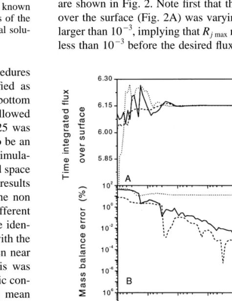
The infiltration problem in Test 1 was simulated again, but this time with the upper boundary condition specified as a known flux. The first simulations of this test showed a strongly fluctuating MBE even for small variations of the maximum allowed residual (Rj max). For that reason, the
infiltration event was simulated repeatedly with all three procedures and with values of Rj max that were decreased
in small steps from 1 to 10¹7. The results at time equal to 5 are shown in Fig. 2. Note first that the time integrated flux over the surface (Fig. 2A) was varying for values of Rj max
larger than 10¹3, implying that Rj maxmust be specified to be
less than 10¹3before the desired flux is imposed correctly.
Fig. 1. Test 1: water content profiles for an infiltration event
simulated with the upper boundary condition given as a known water potential. The solid lines represent simulated results of the three procedures and the dotted line represents an analytical
solu-tion by Ross and Parlange.19
Fig. 2. Test 2: infiltration into the soil from Test 1, but now
simulated with the upper boundary condition given as a known flux. Three characteristic parameters are shown as a function of
The MBE (Fig. 2B) for the non mass-conserving procedure P3 reached a minimum of 13% and stayed constant for decreasing values of Rj max. The MBE for the two
mass-conserving procedures P1 and P2 continued to decrease as expected for decreasing values of Rj max. As mentioned
above, pronounced fluctuations in MBE were seen for both P1 and P2, underlining the importance of using rela-tively small values of Rj max for both procedures. The
number of total iterations used (Fig. 2C) in the two mass-conserving procedures is significantly different. On average, P1 used more that 300 times more iterations than P2 in the simulation of this infiltration event. Except for the largest values of Rj max(which gave an incorrectly imposed flux),
the procedure P1 attempted to find a convergent solution in the very first part of the infiltration event operating with a time step of 0.00005 (the minimum allowed value). The initial guess given by the Euler step (eqn (2)) was used as the solution in almost all these time steps. Later in the infiltration event, the time step was gradually increased to 0.05 (the maximum value) for the rest of the simulation. This observed problem of P1 in obtaining convergence when steep gradients are present, has also been reported for the substantially identical scheme investigated by Johnsen et al.11 Similar problems were not seen in the procedure P2.
3.3 Test 3
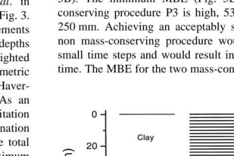
In a more demanding test, a layered soil column was structed and simulated with highly dynamic boundary con-ditions for a period of one full year. The constructed soil column consisted of two layers of Yolo Light Clay8and one layer of sand.8The hydraulic properties for these two mark-edly different soil types are given by Haverkamp et al.8in the form of analytical expressions, and are shown in Fig. 3. The soil column and the separation into depth increments (control volumes), which increase steadily for depths greater than 44 cm, is shown in Fig. 4. The weighted hydraulic conductivity was calculated as the geometric mean (Kj¹1=2¼(Kj¹1Kj)1
=2), as recommended by
Haver-kamp and Vauclin7 and Schnabel and Richie.20 As an upper boundary condition, measured values of precipitation with a time resolution of 3600 s were used in combination with a constant evaporation of 500 mm year¹1. The total precipitation equaled 548 mm year¹1, and the maximum value on a hourly, daily and weekly basis equaled 4 mm h¹1, 21 mm day¹1 and 47 mm week¹1, respectively. As a lower boundary condition, a fixed soil water potential of 0 cm was used (i.e. a fixed water table). In P1, the time step was allowed to vary between 3.6 and 3600 s, which is equivalent to that used by Ahuja et al.,1and a fixed time step of 3600 s was used in P2 and P3. In a series of additional simulations with P1, different numbers of iterations were tried before reducing the time step. With values of this input parameter of 25, 50, 100 and 200, the following total number of iterations for simulating the full year was found to be 803 000, 697 000, 710 000 and 997 000 (Rj max¼
10¹12m s¹1). Based on this, 50 iterations were chosen as an optimal number of iterations before the time step was set back. The optimal factor for increasing the time step in P1 was determined in a similar analysis. With values of this factor of 1.05, 1.1 to 1.2, the numbers of total iterations was calculated to be 829 000, 697 000 and 760 000 (Rj max ¼
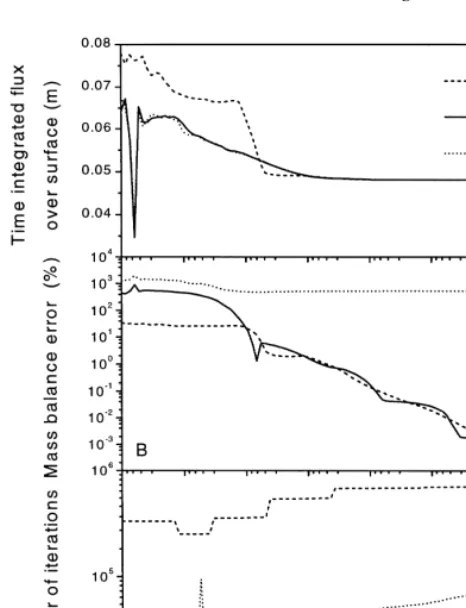
10¹12m s¹1), based on which a factor of 1.1 was chosen. As in Test 2, the year was simulated repeatedly with varying values of Rj maxand the results for all three procedures are
shown in Fig. 5.
The calculated soil water potential at the top of the upper clay layer varied between ¹3.8 and 0.71 m, while the variation in the top of the sand layer was between ¹0.90
and¹0.50 m. Note first that a relatively small value of Rj max
was needed before the desired net flux was imposed and an acceptable small MBE (eqn (16)) was achieved (Fig. 5A and 5B). The minimum MBE (Fig. 5B) for the non mass-conserving procedure P3 is high, 530%, corresponding to 250 mm. Achieving an acceptably small MBE using this non mass-conserving procedure would require extremely small time steps and would result in excessive calculation time. The MBE for the two mass-conserving procedures P1
Fig. 3. Soil water content (A) and hydraulic conductivities (B) for
the two markedly different soils used in Tests 3 and 4: the Yolo Light Clay and a sand soil (after Haverkamp et al.8).
Fig. 4. Inhomogeneous deviation into control volumes of the soil
and P2 was of the same order of magnitude for relevant values of Rj maxand continued to decrease as expected for
decreasing values of Rj max. The number of iterations used
(Fig. 5C) for the two mass-conserving procedures was significantly different. On average, P1 used 19 times more iterations than P2 to simulate this highly dynamic infiltra-tion event. This large difference is partly caused by reduc-tions in time steps in P1 in order to aid convergence, which happened in seven situations through the simulated year when a relatively dry top soil was exposed to precipitation. In three situations the time step was cut back to values between 450 and 1800 s, and in four situations the time step was set back to the minimum allowed time step of 3.6 s and kept there for a short period of time. The initial guess given by the Euler step (eqn (2)) was used as the solution in some of these time steps. The difficulties of P1 in obtaining convergence when steep gradients are present was not seen for P2. It should be noted that no difference between the numerical solutions of P1 and P2 was observed. Comparing the total number of iterations used for P2 and P3 shows that mass conservation can have a stabilizing effect on the iteration process. The full year was simulated in 183 s with P1 and in 10 s with P2 on a Pentium/233 MHz personal computer (Rj max¼10¹12m s¹1).
3.4 Test 4
In this test the ability to handle source terms was compared for the two mass-conserving procedures. The starting point was the same problem as simulated in Test 3, but now simulated with the upper boundary condition specified as a known water potential. This water potential at the top of the soil that was calculated in Test 3 (with P2) was stored with one value per hour of simulated time and used as an input in this test. As shown below, this boundary condition gave very similar performances for P1 and P2 when the source term equaled zero. The function in the SOIL model9for water uptake by roots was used as an example of a source term. The function is given by the following equations, and shown on Fig. 6A
log(¹100w)#2:3 : S¼Smax18 (18)
2:3,log(¹100w)#4:1 : S¼Smax wc
w
b
4:1,log(¹100w)#4:2 : S¼Smax
wc
wcc
b
(42¹10 log(¹100w))
where b ¼ 0.5, log(¹100wc)¼2:3, log(¹100wcc)¼4:1
and Smaxis the water uptake in a wet soil.
In addition to the explicitly included source term in P1, an implicitly imposed source term in P1 also was tested. The year was simulated repeatedly with increasing values of Smax
and a constant value of Rj maxof 10¹12m s¹1. The results are
shown in Fig. 6B.
Note first that the numbers of iterations used in the two procedures were almost identical for Smaxequal to zero. For
increasing values of Smax until a value of approximately
0.006 cm3cm¹3day¹1was reached, the number of iterations used in P1 increased evenly, whether the source term was imposed implicitly or explicitly. For larger values of Smax,
Fig. 5. Test 3: 1 year simulation of the layered soil where the
upper boundary condition is given as a highly dynamic flux. Three characteristic parameters are shown as a function of the stop
cri-terion in the iteration processes.
Fig. 6. Test 4: 1 year simulation of the layered soil where a source
term is specified. (A) The dependency between the source term and soil water potential (after Jansson9). (B) Number of iterations
the implicitly imposed source term caused divergence (number of iterations .2 000 000), and it was only possible to find a solution with P1 if the source term is imposed explicitly. The number of iterations continued to increase for P1, and at Smaxequal to 0.01 cm3cm¹3day¹1, the total
increase equaled a factor of 13. At several instances the time step was reduced in P1 in order to aid convergence, but only to a minimum value of 1400 s when the source term was imposed explicitly. A much smaller increase equal to a factor of 1.6 was observed for P2 when Smaxvaried from 0
to 0.01 day¹1, compared to the factor of 13 for P1.
4 CONCLUSION
The test results show clearly that the mass-conserving pro-cedures P1 and P2 are superior to the non mass-conserving procedure. Mass conservation can be obtained without any cost in terms of a more complicated implementation, less flexibility, or increased calculation time. In fact, mass con-servation seems to have a stabilizing effect on the iteration process (see Fig. 2C and Fig. 5C).
In terms of implementation, P1 is slightly more compli-cated to compute than P2. This is primarily due to (1) the possible change in time steps in P1 where an ongoing itera-tion process is terminated and started again with a smaller time step, and (2) the Euler step, which is used as an initial guess in every time step, or in extreme situations, as a solu-tion when a convergent solusolu-tion cannot be found. As a result of the gradually increasing underrelaxation technique, P2 works more simply with a fixed time step and where no initial guess is calculated. Furthermore, no substituting solu-tion is needed for P2, since the gradually increasing under-relaxation technique will always lead to a convergent solution. This may seem to be a rather arbitrary postulate, but P2 has been tested extensively and divergence has never been observed. It should also be noted that all tests pre-sented in this paper are based on a maximum value of the underrelaxation factor (am) of 0.9, which easily can be given a higher value to increase stability.
The observed differences in performance between the two mass-conserving procedures are strongly dependent on the type of boundary condition specified. In all situations where no source terms were involved, and where boundary conditions were given as known water potentials, the number of iterations needed to find a solution was similar for P1 and P2. In more challenging situations, where fluc-tuating boundary conditions were specified as known fluxes, P1 and P2 performed very differently. In these situations, the time step was occasionally set back in P1, resulting in a large number of iterations used per unit time. The gradually increasing underrelaxation technique allowed P2 to work with the same time step without any noticeable increase in the number of iterations used to find a solution. This resulted in a significant difference (a factor of 300 in Test 2 and a factor of 19 in Test 3) between the iterations needed in the two procedures. The two different approaches for including
source terms in P1 and P2 also have a large impact on the performance of the two procedures. The explicitly formu-lated source term in P1 slowed the rate of convergence for this procedure much more than the approach in P2. This approach also allowed the source term to be included impli-citly, which corresponds to the rest of the implicit scheme. The differences in performance between the two mass-conserving procedures P1 and P2 are particularly important in long-term simulations of realistic field situations where calculation time can be crucial.
REFERENCES
1. Ahuja, L. R. & Hebsom, C., Root zone water quality model. GPSR Report 2, USDA, Agriculture Research Service, Fort Collins, CO, 1992.
2. Allen, M. B. and Murphy, C. L. A finite-element collocation method for variably saturated flow in two space dimensions.
Water Resour. Res., 1986, 22, 1537–1542.
3. Celia, M. A., Bouloutaas, E. T. and Zarba, R. L. A general mass-conservative numerical solution for the unsaturated flow equation. Water Resour. Res., 1990, 26, 1483–1496. 4. Celia, M. A., Ahuja, L. R. and Pinder, G. F. Orthogonal
collocation and alternating-direction procedures for unsatu-rated flow problems. Adv. Water Resour., 1987, 10, 178–187. 5. Cooley, R. L. Some new procedures for numerical solution of variably saturated flow problems. Water Resour. Res., 1983,
19, 1271–1285.
6. Hansen, S., Jensen, H. E., Nielsen, N. E. and Svendsen, H. Simulation of nitrogen dynamics and biomass production in winter wheat using the Danish simulation model DAISY.
Fert. Res., 1991, 27, 245–259.
7. Haverkamp, R. and Vauclin, M. A note on estimating finite difference interblock hydraulic conductivity values for tran-sient unsaturated flow problems. Water Resour. Res., 1979,
15, 181–187.
8. Haverkamp, R., Vauclin, M., Touma, J., Wierenga, P. J. and Vachaud, G. A comparison of numerical simulation models for one-dimensional infiltration. Soil Sci. Soc. Am. J., 1977,
41, 285–294.
9. Jansson, P.-E., Simulation model for soil water and heat conditions. Description of the SOIL model. Tech. Rep. 165, Swedish University of Agricultural Sciences, 1991. 10. Jansson, P.-E. & Halldin, S., Soil water and heat model.
Technical description. Swedish Coniferous Forest Project. Tech. Rep. 26, Swedish University of Agricultural Sciences, 1980.
11. Johnsen, K. E., Liu, H. H., Dane, J. H., Ahuja, L. R. and Workman, S. R. Simulating fluctuating water tables and tile drainage with Modified root zone water quality model and a new model WAFLOWM. Trans. ASAE, 1995, 38, 75–83. 12. Johnsson, H., Bergstroem, L., Jansson, P.-E. and Paustian, K.
Simulated nitrogen dynamics and losses in a layered agricul-tural soil. Agric. Ecosyst. Environ., 1987, 18, 333–356. 13. Milly, P. C. D. Advances in modeling of water in the
unsaturated zone. Transport in Porous Media, 1988, 3, 491–514.
14. Milly, P. C. D. A mass-conservative procedure for time-stepping in models of unsaturated flow. Adv. Water
Resour., 1985, 8, 32–36.
16. Parlange, J.-Y., Barry, D. A., Parlange, M. B., Hogarth, W. L., Haverkamp, R., Ross, P. J., Ling, L. and Steenhuis, T. S. New approximate analytical technique to solve Richards’ equation for arbitrary surface boundary conditions.
Water Resour. Res., 1997, 33, 903–906.
17. Patankar, S. V., Numerical Heat Transfer and Fluid Flow. McGraw Hill, New York, 1980.
18. Richards, L. A. Capillary conduction of liquids through porous mediums. Physics, 1931, 1, 318–333.
19. Ross, P. J. and Parlange, J.-Y. Comparing exact and numer-ical solutions of Richards’ equation for one-dimensional infiltration and drainage. Soil Sci., 1994, 157, 341–344. 20. Schnabel, R. R. and Richie, E. B. Calculation of internodal
conductances for unsaturated flow simulations: A com-parison. Soil Sci. Soc. Am. J., 1984, 48, 1006–1010. 21. Warrick, A. W. Numerical approximations of darcian flow
through unsaturated soil. Water Resour. Res., 1991, 27, 1215–1222
APPENDIX A
The numerical scheme in procedure P2 is derived below using a straightforward control volume approach.17 This approach has been used in solving a wide range of extremely complicated problems in the field of modeling fluid flow and heat transfer, and it can also be applied to water movement in soils. One attractive characteristic of the control volume formulation is that it has some intuitive advantages over the finite difference and finite element methods, which makes it easier to evaluate each of the discrete approximations that together form the numerical procedure.
Using the control volume formulation, the soil column is divided into a finite number of non-overlapping control volumes, each containing a grid point at its center. It is assumed that the variation in space and time of the relevant variables is described by piecewise continuous profiles, which are uniquely determined when the grid point values of the variables are known. A general discretization equa-tion is then derived using these profiles in an integraequa-tion of Richards’ equation18over a time step and a control volume. The starting point is Richards’ equation where a source term is included
The left side of eqn (A1) can be expressed as
]v
where dv=dwis the specific water capacity.
The source term is in many practical applications a non-linear function of the dependent variable w and it is an advantage to directly include at least some of this dependency by expressing S as a linear function ofw
S¼ScþSpw: (A3)
The general technique for linearizing the source term (cal-culate values of Scand Sp) for a given dependency between S andwis outlined below.
Inserting eqns (A2) and (0) in eqn (A3) and integrating the result over the time step from time t to tþDt and over
It is now assumed that dv=dw is constant throughout the
time step and that the grid point values of dv=dw, ]w=]t, Scand Spwprevail throughout the control volume as
repre-sentative mean values. These assumptions lead to
dv
The two first terms in the time integral in eqn (A5) express the Darcy fluxes out and in of the control volume. Assuming that Kj¹1 prevails throughout control volume j ¹ 1, that Kj prevails throughout control volume j, and
that quasi-stationary conditions are present, the flux qj¹1=2
over the surface of j¹1=2 can be expressed exactly as
qj¹1=2¼ ¹Kj¹1
wherewj¹1=2is the soil water potential at the surface
separ-ating the two control volumes. Eliminsepar-ating wj¹1=2 from
eqn (A6) gives
Kj¹1=2 is the weighted hydraulic conductivity calculated as
the well-known harmonic mean, where a non-uniform separation of a soil column into control volumes is taken into account. A large selection of different weighting pro-cedures exist and have been tested and compared in several studies.7,20,21 In general, the geometric mean (Kj¹1=2¼(Kj¹1Kj)
1=2
Inserting eqn (A7) and the equivalent expression for
In the approximation of the time integral, it is necessary to assume how all the time-dependent terms are varying from time t to tþDt. In general, the time integral of Kjþ1=2wjþ1,
for example, can be expressed as
ZtþDt
t Kjþ1=2wjþ1dt
¼((1¹b)Kjnþ1=2wjnþ1þbKjnþþ11=2w nþ1
jþ1)Dt ðA10Þ
where b is a weighting factor. Different known schemes can be obtained depending on the value ofb. Settingb¼0 gives an explicit scheme,b¼1/2 leads to the well-known Cranck–Nicolson scheme, and b ¼ 1 gives an implicit scheme. Here, the implicit scheme is chosen by which eqn (A9) yields
The essential element in achieving mass conservation is the approximation of(dv=dw)j. In order to guarantee mass con-servation in the numerical solution, it is necessary that the principle of conservation is expressed exactly in the dis-crete formulation as it is in the differential formulation. The control volume approach leads to a simple balance (a change in water content equals a difference in fluxes) expressing the principle of conservation. Consider a time step where a certain change in water content is calculated for a control volume. In a ‘reverse’ time step, imposing the opposite directed fluxes in and out of the control volume should lead to the same numeric change in water content. This will not be the case using the standard implicit finite difference approach, where (dv=dw)j is evaluated at time
tþDt.
The appropriate approximation of(dv=dv)jcan be derived by integrating eqn (A2) as before over the time step from
time t to tþDt, and over the control volume j, from zj¹1=2to constant throughout the time step and that the grid point value of dv=dw prevails throughout the control volume as
representative mean values. With these assumptions, eqn (A12) gives
This result is equivalent to the approximation derived by Cooley15and Milly14using a finite element approach.
Letting j vary from 1 to N (the soil column is divided into
N control volumes), eqn (A11) together with eqn (A13)
describes a tridiagonal system of N non-linear equations with Nþ2 unknown values ofwnjþ1. The system of equa-tions will be closed by two additional equaequa-tions expressing the boundary conditions (described below). The non-linear-ity of the equations is overcome through iterations, where values of vnjþ1, Kjnþ1, Sncjþ1 and Snpjþ1 are evaluated from values ofwnjþ1 from the previous iteration step. Using the symbol m for the iteration level, eqn (A11) can be written as
Amj wjn¹þ11,mþ1þBmjwjnþ1,mþ1þCjmwjnþþ11,mþ1¼Dmj
The boundary conditions are introduced by defining two additional and infinitely small control volumes, one on top of the soil surface and one directly below the soil col-umn. These control volumes will be numbered 0 and Nþ1. A Dirichlet condition (a known soil water potential) is assigned as an upper boundary condition by giving the following values to the coefficients in eqn (A14) written for control volume number 0
Bm0 ¼1, C m 0 ¼0, D
m
where wt is the known soil water potential at the upper
boundary. As a lower boundary condition the Dirichlet condition is likewise given by
AmNþ1¼0, B m
Nþ1¼1, D m
Nþ1¼wb (A17)
A Neumann condition (known flux) is expressed as an upper boundary condition by letting j equal one in eqn (A7). Recalling thatDz0 is infinitely small and
substi-tuting q1/2 by qt(the known flux at the boundary) leads to
Bm0 ¼
As a lower boundary condition, the Neumann condition is likewise given by eqn (A15). If the source is independent ofw, it is sufficient only to initiate Sncjþ1,m, and to do this before the first itera-tion step. A source dependent of w can also be included only through Sncjþ1,mbut since the dependency ofwis not directly included, this strategy will in general slow down the convergence. A better strategy is to include the depen-dency ofwthrough Snpjþ1,mwhich will result in a consider-ably faster numerical solution. In general, a source Sj can
be linearized by
Relating eqns (A20) and (A3) gives the following general expressions for Sncjþ1,mand Snpjþ1,m
It is essential that no values of Bmj equal zero in the solution
of eqn (A14). To prevent this, it is necessary to require that all values of Snpjþ1,m are less than or equal to zero (as the first three terms in the expression for Bmj in eqn (A15)).
This requirement is not particularly restrictive, since the relevant processes included through the source term generally have negative values of Snpjþ1,m when they are linearized.
One additional advantage of mass-conserving procedures is that the MBE that is present during the process of finding a convergent solution in any arbitrary iteration step can be calculated exactly and used as a criterion for convergence. Recall that eqn (A14) is a balance between the change in water storage per unit time and the water fluxes in and out of the control volume. Assuming that the coefficients Amj þ1, Bmj þ1, C
mþ1 j and D
mþ1
j are recalculated right after values of
wnjþ1,mþ1are found by solution of eqn (A14), the MBE per unit time for control volume j is equal to
Rjmþ1¼lDmj þ1¹Ajmþ1wnj¹þ11,mþ1¹B
In most situations a converged solution of eqn (A14) is reached in a few iterations. However, sometimes oscilla-tions occur that increase the number of iteraoscilla-tions needed to find a converged solution, or even cause divergence in the iteration process. This can effectively be prevented if an underrelaxation of the values ofwnjþ1,mþ1is done immedi-ately after these values are calculated by solution of eqn (A14). The following expression is used
wjnþ1,mþ1,u¼(1¹am)wjnþ1,mþ1þamwnjþ1,m (A23) where am is the relaxation factor with a value between 0 and 1. Immediately after the underrelaxation is done,
wjnþ1,mþ1 is given the values ofwjnþ1,mþ1,u. It is a good strategy in each time step to first start the underrelaxation after a few iterations because a converged solution most often is found by then. It is also an advantage to start the underrelaxation with a smaller value of am and then increase am with the number of iterations in the actual time step.
The denominator in eqn (A13) can be close to or equal to zero. This will be the situation, for example, if a steady-state solution is found. In order to achieve a realistic numerical representation of (dv=dw)mj under all circumstances,
(dv=dw)mj can be calculated as follows. Assuming that vis
known as the unique relation F ofw, either as a continuous function or as a table where interpolations can be made,
(dv=dw)mj can then be calculated effectively by
where the function SIGN equals 1 or ¹1, depending on the sign of the argument, the function MAX equals the maximum value of the two arguments, and Dwmin is the
predefined minimum numeric values of the denominator (SIGN and MAX are standard functions in most program-ming languages). Note that iflwnjþ1,m¹wnjlis greater than
Dwmin, eqn (A24) is identical to eqn (A13).
The entire solution procedure in any arbitrary time step is summarized below:
(A15), (A16), (A17), (A18) and (A19) and values for Kjn¹þ11,=2m, (dv=dw)
m
j , Sncjþ1,m and S nþ1,m
pj from the
2. Findwnjþ1,mþ1 by solution of eqn (A14). Underrelax the values of wnjþ1,mþ1 using eqn (A23) if m is greater than a predefined number.
3. Calculate values of Kjnþ1,mþ1andvnjþ1,mþ1based on
wjnþ1,mþ1. Calculate values of Kjn¹þ11=,2mþ1 using the
geometric mean, and values of (dv=dw)mj þ1 using eqn (A24). Calculate values of Sncjþ1,mþ1 and
Snpjþ1,mþ1 based onwnjþ1,mþ1 using eqn (A21).
4. Calculate Amj þ1, B mþ1 j , C
mþ1 j and D
mþ1
j using eqns
(A15), (A16), (A17), (A18) and (A19) and the max-imum value of Rmj þ1 using eqn (A22). If the
maxi-mum value of Rmj þ1 is greater than a predefined