ROBUST SURFACE MATCHING BY INTEGRATING EDGE SEGMENTS
N. Kochi a.b, *, T. Sasaki a, K. Kitamura a, S. Kaneko c
a
R&D Center, TOPCON CORPORATION, 75-1, Hasunuma-cho, Itabashi-ku, Tokyo,Japan – [email protected]
bR&D Initiative, Chuo University, 1-13-27, Kasuga, Bunkyo-ku, Tokyo, Japan
cHokkaido University Graduate School of Information Science and Technology, Kita14, Nishi9, Kita-ku,
Sapporo,060-0814, Hokkaido, Japan
Commission V, WG/4
KEY WORDS: Surface matching, 3D, Edge, Line segment, Parallax estimation, Reconstruction
ABSTRACT:
This paper describes a novel area-based stereo-matching method which aims at reconstructing the shape of objects robustly, correctly, with high precision and with high density. Our goal is to reconstruct correctly the shape of the object by comprising also edges as part of the resulting surface. For this purpose, we need to overcome the problem of how to reconstruct and describe shapes with steep and sharp edges. Area-based matching methods set an image area as a template and search the corresponding match. As a direct consequence of this approach, it becomes not possible to correctly reconstruct the shape around steep edges. Moreover, in the same regions, discontinuities and discrepancies of the shape between the left and right stereo-images increase the difficulties for the matching process. In order to overcome these problems, we propose in this paper the approach of reconstructing the shape of objects by embedding reliable edge line segments into the area-based matching process with parallax estimation. We propose a robust stereo-matching (the extended Edge TIN-LSM) method which integrates edges and which is able to cope with differences in right and left image shape, brightness changes and occlusions. The method consists of the following three steps: (1) parallax estimation, (2) edge-matching, (3) edge-surface matching. In this paper, we describe and explain in detail the process of parallax estimation and the area-based surface-matching with integrated edges; the performance of the proposed method is also validated. The main advantage of this new method is its ability to reconstruct with high precision a 3D model of an object from only two images (for ex. measurement of a tire with 0.14mm accuracy), thus without the need of a large number of images. For this reason, this approach is intrinsically simple and high-speed.
* Corresponding author. This is useful to know for communication with the appropriate person in cases with more than one author. 1. INTRODUCTION
In our previous research works we have developed the “area based matching method” TIN-LSM and applied it to various measurement projects (Kochi, 2009). We have then integrated OCM (Orientation Code Matching, Ulah, et al. 2001) into the system and further developed the method, the extended-TIN-LSM, which is robust to occlusion, brightness change and geometric distortion (Kochi, et al. 2012a).
Thearea based matching works well with objects which have a smooth surface and texture features, such as for example the walls of historical ruins, but it fails with objects which have steep, sharp edges or whose surface has poor texture features, such as for example modern building facades or indoor scenes. The reason resides in the approach of area based matching methods, which set as template the basic image and obtain highly dense and highly accurate results by performing the matching on the corresponding image. However, as a direct consequence of this approach, it becomes not possible to correctly reconstruct the shape around steep edges. Moreover, in the same regions, discontinuities and discrepancies of the shape between the left and right stereo-images increase the difficulties for the matching process.
In order to overcome these problems, we propose in this paper the approach of reconstructing the shape of objects by embedding reliable edge line segments into the area-based matching process with parallax estimation. We propose a robust stereo-matching method which integrates edges and which is
able to cope with differences in right and left image shape, brightness changes and occlusions.
2. RELATED WORKS
Feature based matching processes as the well-known SIFT (Low, 2004), Surf (Bay, et al. 2008) and others detect the most distinctive spots showing features. These methods are robust against rotation, scaling and illumination change. They are suitable matching processes when a large quantity of images is required, as it is the obvious case of Sfm (Structure from motion). However, in regions where features cannot be detected or in regions where the corresponding features cannot be found, a large amount of images is required in order to obtain a reliable configuration (Frukawa, et al. 2009). Feature based matching processes are employed for example in Phototurism (Snavely, et al. 2006) and PMVS2 (Furukawa, 2010), as core methods for producing 3D models out of massive amount of images. Such solutions produce 3D models out of, for example, tourism pictures and create virtual worlds for the viewers to enjoy sceneries and walk-throughs. These techniques are however not available for the reconstruction from images of buildings, which have scarcely features and, even if this would be possible, it would take long time.
On the other hand, Matis Laboratory (IGN France) has developed an open source 3D modeling software based rigorous and accurate photogrammetric methods. This software features two main components; an image orientation tool called APERO
and a dense image matching tool called MicMac (Pierrot, et al. 2011). The MicMac multi image matching process is based on energy minimization using a modified semi-global matching algorithm (Hirschmuuler, 2008). Chiabrando et al. 2013 performed tests on point clouds generation for metric Cultural Heritage documentation by applying the MicMac solution, Terrestrial Laser Scanner and Topcon Image Master (based on TIN-LSM method). The tested area was 45m x 30m wide. Check points were measured by Total Station and used for the comparison. The tests showed that the results obtained by Image Master was less than 1cm accurate and the results obtained by the other methods had accuracies fluctuating around 2cm.
Extended stereo-matching methods which use edge features and line segments as additional information have been largely discussed (Deriche, et al. 1990, Zhang, 1995, Schmid, et al. 1997. Ok, et al. 2011). These methods still present the following challenging problems: (a) When the edge ends and the middle points used for matching are obscure or have noise, or when the corresponding line segments are cut in two or more pieces, it is not possible to obtain the corresponding points; therefore the results are unreliable. (b) When the line segment has only weak restriction in overlapping areas it is not possible to apply strong geometrical constraints; and when the line segment is almost parallel to the epipolar line, it is basically impossible to obtain precisely the corresponding points. Methods which make local matching between the line segments cannot basically solve the problems (a) (b). For this reason, is being studied the method using topological configuration and geometrical constraint by the graph from the plural line segments(Ayache, et al.1987, Horaud et al. 1989, Schmid, et al. 1997). This method groups plural line segments enabling stronger geometrical constraints. It has therefore, the advantage to get over the problems (a) (b) described above. It has however the disadvantage that the segmentation process becomes sensitive to errors, because it becomes more complicated. In Schmid et al. 1997 two cases are differentiated: when the base line is short and when it is long; the former for the process to make locally the matching between the edges and the latter when plural edges are available. When the base line is short, that is, when corresponding points are close, that is, when the direction, length and area of overlapping of each line segments are similar, this method is applied. Moreover, in this case, one additional image is included in the process, thus making with three images a more robust error deletion. This method is however week in case of rotations, scaling and changing of configuration. On the other hand, when the base lines are short, the images tend to be identical between them, and thus this method works well for the tracking of moving images. When the base line is long, this method detects feature points using homography for plural line segments and with the epipolar constraint. By discerning the parameter between the groups nearby, erroneous actions can be reduced.
Bay et al. 2005 apply the geometrical arrangement of plural line segments and homography to delete errors and add increasingly line segments. They try to obtain the epilolar value only at the end of the process, so that this is not required to be known at the outset.
All these methods aim at obtaining the correspondence (matching) of line segments as accurately as possible. On the other hand, our aim is not to obtain the matching between line segments, but to obtain the surface configuration of an object, including the edge features as accurate and dense as possible. In concrete, we use the convenient method of 2D straight-line edge detection (Kochi, et al. 2012b, 2013), which estimates and detects edges with certainty solving the challenge (a) described
above. Regarding the challenges (a) (b), the values of parallax estimation are obtained; this is robust to occlusion and brightness change. Based on these carefully research works we propose our method which aims to attain accurate and speedy detection of 3D edges as configuration of an object.
In this paper we present the extended Edge TIN-LSM method, which integrates the 3D edges into the area based coarse to fine LSM. In chapter 3 we will first explain briefly the method of the edge detection and we present other processes such as parallax estimation, edge-matching, and the edge surface matching. In Chapter 4 we will describe the efficiency assessment.
3. PROPOSED METHOD
In our method, we first make edges into 3D perspective and obtain high accuracy by TIN (Delaunay, 1934). We apply then coarse-to-fine LSM, which is robust to changes of shape (Kochi, et al. 2012a).
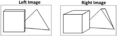
In the 3D perspective obtained in this way, the edges formed by line segments include the straight lines composing the surface, the intersecting lines of adjacent surfaces and the corners where the straight lines meets together. By the representation with these straight lines, the left and right images look different (the shape looks different, see Figure 1). This fact makes difficult to determine corresponding points and can easily cause mismatching points, generating thus instable results. To overcome this problem, uncertain edges are deleted and corresponding points are estimated by OCM (Orientation Code Matching, Ulah, et al. 2001), which is robust to brightness change and occlusion. In this way, we ensure with certainty the matching of detected edges. Our proposed 3D measuring method is therefore not only robust to brightness change, occlusion, as well to shape changes but also it performs with high speed and high accuracy.
Figure 1. Difference of left and right image
3.1 Proposed Matching Process
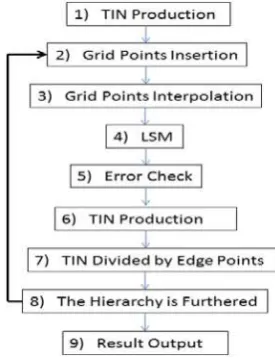
Figure 2 shows the flowchart of our proposed method. The matching process is composed of the following three main parts. Parallax estimation (section 3.2): We use the feature extraction
operator called OCR (Orientation Code Richness, Takauji, 2005) and we apply OCM (Orientation Code Matching). We then remove the mismatching points by the back-matching method and we use the correct corresponding points for the estimation of the value of parallax, which is used for the next step.
Edge-Matching (section 3.3): We detect edges by setting as templates the edge ends and curvature points. Stereo-matching is then applied in the areas delimited by the parallax estimation
Edge Surface Matching (section 3.4): We produce TIN, which shows the parallax from the result of the edge detection obtained from Edge-Matching. Area-based Surface-Matching is then performed with edges grabbed in each search stage within the coarse to fine strategy.
Figure 2. Flowchart of the Extended Edge TIN-LSM
3.2 Parallax Estimation
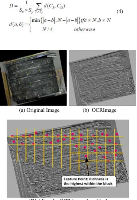
We perform matching on the stereo-image at fixed intervals and calculate the parallax for each block. For the detection of the feature points and for their matching we employ OCR (Orientation Code Richness, Takauji, 2005). We first calculate the OCR image and then divided it into a grid (block) with regular intervals. The OCR image is a representation of the original image showing the areas where are present numerous orientation code features. We detect feature points in the locations where the value of richness is the highest within the generated single blocks and perform matching with the image to compare. Figure 3(a) shows the original image of a tire as an example, (b) is the calculated OCR Image, and (c) shows the division of the OCR image into blocks.
3.2.1 Orientation Code Richness (OCR): We calculate the relative frequency Pxy(i) = hxy(i)/M2 - hxy(N) (i = 0,1,,,,,,,N-1)
with the frequency of the apparition of each OC (Orientation Code) as hxy(i) (i = 0,1,,,,,,,N-1) in a limited local area with size
M by M pixels and centered at the interest pixel (x,y). At this time, since the value of the hxy(N) is the unreliable code for the
low contrast, we leave it out from the relative frequency. As a result, the entropy of OC, 0 ~ N-1, is shown by the following equation.
∑
− == 1
0 ()log2 () N
i xy xy
xy P i P i
E (1)
The maximum value of entropy Emax is Emax = log2N, when each OC goes with uniform distribution Pxy(i) = 1/N. When we
calculate the Richness, therefore, we set the threshold value αe (0<αe<1) and consider the area where the entropy is above αe Emax as the feature area. Thus the Richness Rxy is expressed in
the following equation.
(2)
3.2.2 Orientation Code Matching (OCM): If we determine the intensity at the pixel coordinates (x,y) of an object as I(x,y), the intensity gradient on the horizontal axis as ΔIx = ∂I/∂x and
the intensity gradient on the vertical axis as ΔIy = ∂I/∂y, we can
then obtain the orientation angle of the interest pixel as θ(x,y) = tan-1(ΔIy/ΔIx). In this study we used Sobel operator (Sobel,
1978) to calculate the gradient value. The Orientation Code is the quantized value of the orientation angle θ within the proper quantization width Δθ = 2π/N. Its equation is expressed as follows.
(3)
We quantize the periphery of a circle by N parts, the OC is shown as 0 ~ N-1. “Γ” is the threshold value defined to obtain OC in stable manner and in case of low contrast we put N as the unreliable code. In our study we divided the periphery by 16 directions (N=16). If we give the name “O” to the original image, to which the other image “R” is referred, both having the same size Sx x Sy, and if we make the OC Image from both of
them as CO, and CR, by using equation (3), the following will be
the relevant equation, in which the mean of absolute residuals “D” works as the verification value of the absolute difference criterion values “d”.
(4)
(a) Original Image (b) OCRImage
(c)Dividing the OCR image into blocks
Figure 3. Feature points detection from OCR image ISPRS Annals of the Photogrammetry, Remote Sensing and Spatial Information Sciences, Volume II-5, 2014
3.3 Edge Matching
3.3.1 Edge Detection: Especially edge corners appear with different shapes in the right and the left images; this fact often results in deterioration and mismatching. In order to make the matching process stable, we delete the problematic corners, we detect the edge ends and we connect them with a straight line, identifying it as the edge-line segment. We have thus developed a new method to detect edges. In our new method, we delete corners with values over 30 degrees and identify corners with lower values than this threshold as curvature points.We use the Sobel filter to detect edges.
The “Edge-Line-Segment-Detection” method is expressed in equation (5), with fx and fy as differential in X axis and Y axis direction, using edge strength It and edge length Len as assessment value.
) (
; ) (
max Len1 x2 y2
i Iti It f f
It
k⋅ <∑= = + (5)
Since the length of the edge line segmentneeds at least more than 3 pixels, we have chosen the value 5 and we have defined edges the ones having five times (=k) more than the highest edge-strength It. In this method, we consider the length of the edge line segment and the edge-strength as the assessment values. In this way we can detect edges which are robust against noise and which are accurate in straight line quality. Moreover this method has the important feature of not detecting sharp corners (Kochi, 2012b, 2013).
3.3.2 Edge Matching (end points, curvature points): Figure 4 shows how we estimate the parallax in the edge matching process. We first identify three points to catch the parallax value which we have obtained by equation (4). We then calculate the weight based on the distance from the edge end-point F and set it as the parallax S (equation (6)).
We use the value of S to delimitate the search area. In this way, we can speed up the process and at the same time reduce the number of mismatching points. Therefore, we can perform highly reliable edge-matching.
We identify and use theedge as 3D Edge only if the matching was successful in all the necessary items, such as the end-points and the curvature points.
∑ −
= n
Sn Ls
Ln Ls S
2 (6)
Here, Sn: Parallax of Feature points Pn, Ls: Sum of Distance, Ln: Distance from F to Feature Points Pn
Figure 4. Parallax estimation
3.4 Edge Surface Matching
In our proposed method, we consider the edge end-points and curvature points obtained in the Section 3.3, and perform the matching in a coarse to fine procedure. The production of TIN is done on the original image and projected on the compressed image of each strata to perform stereo-matching. In our method, the strata number m is the number of the frequency of our dividing by 2 until the vertical sensor pixel number V goes down to 32 (V/2m≦32). The measurement interval pt has to be set depending on the object as demanded by the manual operation. The measuring area where the matching is performed, is set as the external rectangular area surrounding the obtained edge end-points; and we calculate the parallax ds of its center coordinate. With the camera distance from the measurement interval pt and the parallax ds to the right and the left camera as B, and as this is a stereo-image, we determine the measurement interval pt(m) as pt(m) = pt×ds/B×2m.
The flowchart of Figure 5 explains the Edge Surface Matching.
Figure 5. Flowchart of Edge Surface Matching
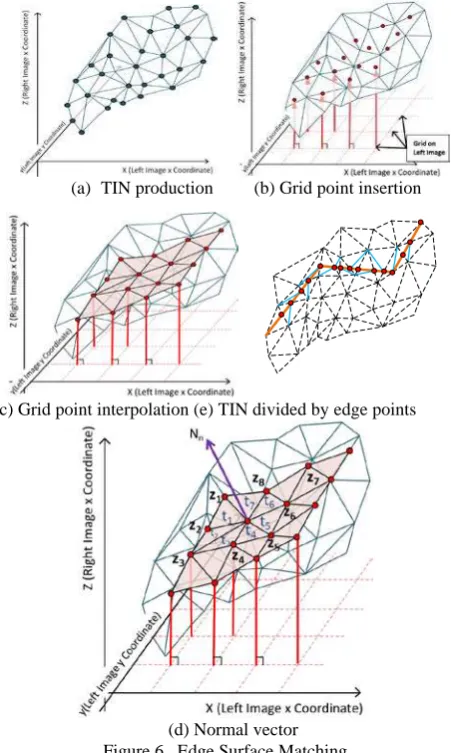
1) TIN production: First, if we have already edge end-points or some other measured point, we produce TIN by incorporating them. As shown in the Figure 6(a) ~ (d), we define the axes as follows: x and y axes represent the x and y coordinates in the left image, the z axis represents the x coordinate in the right image.The difference between the x coordinates of the left image and the x coordinates of the right image is the parallax. Therefore, the TIN represented in the figure shows the parallax projected on the space. The produced TIN would look slant as in the Figure 6(a).
2) Grid Point Insertion: As shown in Figure 6(b), we create a grid in the left image with the same spacing pt(m)and we project the intersecting points of the grid perpendicularly to TIN produced in 1).
3) Grid Point Interpolation: By the projection performed in 2) we can obtain the z coordinate on TIN and insert the grid points as the points of 3D coordinates. We then produce again TIN (Figure 6(c)). This new TIN expresses the corresponding relation between the left and the right images, as well as the parallax.
4) LSM: We perform LSM (Grun, 1985) after producing the template around the vertex of TIN (by intersecting the point of grid on the basic image) generated in 3). LSM is the method which find recursively the parameters of the affine transformationso that the residual r(i,j) of the brightness difference would be minimized(equation (7), whereq(i,j)is
the template and f(x,y) the searching area). This method is robust against geometrical transformations. Its sensitive part regards the initial values which have to be set. This fact is very important because as the matching is performed by changing the parameters of the affine transformation to optimize the result, too much time would be spent to converage to a final result if the initial values are not set correctly.
In our proposed method, we work with rectified images; in this special case, LSM can be expressed as a one-dimensional search. We determine thus a0 - a2 of the equation (8) and a2
becomes the position of the corresponding points on the epipolar constraint.
(7)
(8)
In our method, we estimate the initial values for LSM by TIN of grid points generated in 3). We calculate the normal vector (Nn of the Figure 6(d)) of the top of TIN as the average value
of the normal vectors of the adjacent surfaces (Figure 6(d) t1 -
t7). We change the searching area in accordance to the
inclination of the normal vector of the obtained top. We then perform stereo-matching on the epipolar line and we search for the corresponding points which minimize the sum squares of the difference of grey value (D’Apuzzo, 2003). This process is performed for all the grid points.
5) Error Check: We place the points obtained in 4) on TIN produced in 3), and compare it with the height of the surrounding points (Figure 6(d) z1 - z8). If the value (parallax) is drastically different from the value of the surroundings we mark it as error and remove the point. If we set the obtained point as z0, we determine what satisfies the equation (9) as the detecting location.
8 ~ 1 0
8 ~
1 max
minz ≤z ≤ z (9)
6) We produce TIN with the corresponding points obtained in the processes 1) - 5).
7) We lay the edges obtained in the Section 3.3 one on top of the others. If an edge crosses over a triangle, we add points to the intersecting points of the triangle and the edge, and we further split the triangle from the points we added (Figure 6(e)). With this process it is possible to the boundary of TIN accurate.
8) One step further is made in the search process by increasing the resolution (2 times more in this presentation) of the picture with the grid pt(m-1) = pt(m) /2.
The same processing steps 2) - 8) are then repeated as above and after completion we output the result as solution.
As the process is formed with strata, the parallax (z value of TIN) of the points inserted at 3) and the accuracy of shape estimation by LSM of 4) improve by each stage. Hence, we can obtain a very accurate 3D measurement. Moreover, the structure of the edge boundary enables TIN to have clear borderlines in each stage.
4. EFFICIENCY ASSESMENT
In order to assess the parallax estimation, the effect of the extended Edge TIN-LSM method and thegeneral efficiency of whole system, we applied the proposed method to the measurement of three kinds of tires.
4.1 Parallax Estimation
We compared the number of mismatches resulting by applying with different sizes of the template windows OCM (our proposed method) and NCM (normalized cross-correlation method).
The tire 1 (Figure 7) has an area size of 235 × 90 mm (with groove depth of 10mm); the number of matching points is 211. The tire 2 (Figure 8) has an area size of 190 × 190 mm (with groove depth of 20mm); the number of matching points is 361. The table 1 shows that by increasing the size of the template window, OCM become more stable, because the number of mismatches decreases and is 0 by size the 41. With NCM the number of mismatches varies, depending on the size, and is never getting to 0.
Figure 7 shows the results of the matching process for the tire 1, with the template window of 11 × 11 pixels. The Figure 7(a) shows the results of OCM and the Figure 7(b) of NCM, the blue + signs represents the matched points. Figure 7(c) shows the texture image with NCM matched points, the large yellow + signs represents the mismatches.
From the Figure 7(a) we can note that OCM got matching points evenly and from the Figure 7(b) that NCM got mismatched in the groove area. From these results we can affirm that OCM is more robust than NCM in terms of the template window size, the brightness change and occlusion (groove area).
(a) TIN production (b) Grid point insertion
(c) Grid point interpolation (e) TIN divided by edge points
(d) Normal vector Figure 6. Edge Surface Matching
(a) OCM (b) NCM (c) NCM (mismatches)
Figure 7. Matching points (Tire1)
Template 7 11 21 41
Tire 1 2 1 2 1 2 1 2
OCM 7 6 0 3 0 1 0 0
NCM 10 18 5 14 5 9 24 143
Table 1. Number of mismatches
4.2 Edge Surface Matching
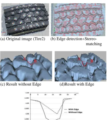
We tried to find whether it is possible to show clearly the structural features of a tire with deep groove. By applying our method, we obtained 144,991 points separated from each other by 1mm. Figure 8(a) shows the original image. On the surface of tire we can see the color-coded targets (Moriyama, et al. 2008) used for orientation. Figure 8(b) shows the result of the stereo-matching process overlapped with the results of edge detection. Figure 8(c) shows the surface of the tire reconstructed with the matching results without edge and Figure 8(d) shows the results obtained by our new method of the edge-surface matching by detecting 3D edges. Figure 8(e) shows a profile line for each method; here we can clearly see that the feature of the groove can be obtained correctly by our proposed method, whereas it cannot be obtained by the method without edge.
(a) Original image (Tire2) (b) Edge detection+Stereo- matching
(c) Result without Edge (d)Result with Edge
(e)Result of measurement compared with surface matching
Figure 8. Measurement result
4.3 Accuracy Assessment
In order to assess the measurement accuracy obtained by our method, we used a contact 3D measuring device (Zeiss UMC550S: 10μm accuracy) on the tire 3 (Figure 9(a)) in order to obtain an unbiased 3D reference data. We applied our proposed method on the stereo-images of the same tire and performed the surface measurement procedure. We then compared the cross sections of the results (Figure 9(a) A-B and A’-B’). These two measurements are different in regards of the measuring method, and the place and time of the performed measurement process was different. For this reasons, we compared the two surfaces by analyzing profiles in areas which we deemed more or less equal.
We mounted a 35mm lens to a Nikon SLR camera and took stereo-image with the photographing distance of 618mm and the base length of 240mm. The achieved resolution for this work was Δxy: 0.1mm for plane and Δz: 0.26mm for depth. Comparing the results with the contact measuring device had some limitations: some areas could not be measured by our device, for example, a narrow groove (width 1~2mm), where one side of the wall surface was not taken in the picture.
For the measurement, we set the measurement pitch of the contact measuring device to 1mm. However, the diameter of the ball at the tip of the probe was 1mm, causing limitations for the tire’s groove width. For this reason, as we could not trust the measuring value around the groove periphery, we deleted these parts from the resulted data. For the comparison we detected and assessed the data with a points spacing 2mm, from the part of 100mm of the line 1 and line 2. The table 2 shows the comparison results. For the line 1 the average was 0.09mm, standard deviation was 0.1mm and maximum difference was 0.4mm. For the line 2 the average was 0.14mm, standard deviation was 0.14mm, maximum was 0.5mm.
While in the generally used method, the groove measuring gage of tire is ±0.1mm for single point measurement, in our proposed new method, we can measure entire surface parts and additionally perform the evaluation of tire wear.
Table 2. Accuracy assessment
(a) Evaluation line (Tire 3)
(b) Comparison between contact 3D measuring device and edge surface matching
Figure 9. Accuracy assessment
A A
B B
4.4 Processing Speed
For our tests we used a part cut out from the tire 3, as shown in the Figure 9(a) and measured it. We produced TIN with measurement spacing of 1mm for the processed area of 200mm×200mm. The number of obtained triangles was 150,000. The stereo-image (rectification image) size was about 3000×3000pixel. The specifications of the PC used for processing the data were the following: Intel Core i7-2640M (core: 2, thread: 4), with 2.8GHz (turbo boost: 3.5GHz). We optimized our software by parallelization of the processes. Especially relevant was the part performing LSM, which is computational heavy and therefore required long processing time. By this optimization (increasing the number of threads from 1 to 4), we could reduce the processing time from 660 seconds down to 90 seconds, which is 7 times faster.
This is fast enough for off-line processing, however faster speed is necessary for real time processing. We are now improving the process in order to speed it up even more, especially the part performing error checks which is difficult to implement through parallelization.
5. APPLICATION
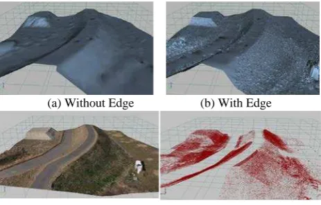
With our proposed method, we can perform 3D measurements and generate 3D surface models in robust way. In this section we demonstrate its application on objects larger than a tire. For the first example, we took aerial pictures of an area (50m × 50m) from 30 meters elevation by using an UAV.
Figure 10(a) shows the result obtained by stereo-matching (Extended TIN-LSM: without edge), using 157 images with the additional texture-mapping. Figures 10(b), (c) and (d) show the result obtained by the proposed method extended Edge TIN-LSM. Figure 10(c) shows the result of the texture-mapping and figure 10(d) shows the result of 3D edge detection. As you can see, in the result obtained by the method without edge (Figure 10(a)) the features are not so clear, while, as shown in Figures 10(b) and (c), the features are clear in the results obtained with the new proposed method.
Figure 11 shows the results obtained on a stair-case. In this case, the data set is composed of 25 pictures acquired from 15 meter elevation (Anai, et al. 2012). We can see clearly the features in the results obtained by the proposed method (Figure 11(b) and (c)), whereas these are not visible in the results obtained by the method without edge (Figure 11(a)).
The last example is shown in the Figure 12, where you find an architectural structure measured by the method without edge and by our new proposed method. Figure 12(a) shows the original image, (b) the textured results obtained by the proposed method, (c) the details of the upper part obtained by the method without edge, (d) the details of the upper part obtained by the method with edge (our new method), (e) the results of the 3D edge detection, (f) the results of the 3D edge detection superimposed on the results of (d). In this example we can see that by the method without edge we cannot express the detailed design of the architectural object, which on the other hand we can do with the extended Edge TIN-LSM method.
6. CONCLUSION
We have developed and proposed the extended Edge TIN-LSM method which is a robust surface measurement method with integrated edges. Our method uses OCM to estimate the parallax, because of its robustness against brightness change and occlusions. Edge line segments are detected directly and edge matching is performed with high precision.
(a) Without Edge (b) With Edge
(c)Texture mapping with Edge (d) 3D Edge Figure 10. Measurement by UAV
(a) Without Edge (b) With Edge (c) 3D Edge
Figure 11 Measurement result of stair-case
(a) Original image (b) Proposed method
(c)Without Edge (upper part) (d) With Edge (upper part)
(e) 3DEdge (f) 3DEdge+Surface
Figure 12. Measurement result of an architectural structure
The 3D edges thus obtained are integrated into the stratified TIN by performing LSM, which is robust against changes of shape. In this way we finally realize a shape expression, which was not possible before with area-based matching. The precision we attained was as high as 0.14 mm when we applied our method to the measurement of tires. Furthermore, as we have implemented the method in a parallel high speed procedure, we could shorten the processing time from 660 sec down to 90 sec to perform the high density, high accuracy and high speed measurement of this area.
The main advantage of this new method is its ability to reconstruct with high precision a 3D model of an object from only two images, thus without the need of a large number of images. For this reason, this approach is intrinsically simple and high-speed.
(c) Texture mapping with Edge (d) 3D Edge
Figure 10. Measurement by UAV ISPRS Annals of the Photogrammetry, Remote Sensing and Spatial Information Sciences, Volume II-5, 2014
Further works will be made on the matching between edges in the architecture of fewer features and on the method to perform matching on the basis of data of the surface, which constitute the edge.
We will continue the challenge to ameliorate our method and to apply it to every possible object.
References
Delaunay, B., 1934. Sur la Sphere Vide. Bull. Acad. Sci. Mat. Nat., pp.793-800 .
Sobel, I., 1978. Neighbourhood coding of binary images for fast contour following and general array binary processing, Computer Graphics and Image Processing, vol.8, pp.127-135.
Grun, A., 1985. Adaptive Least-squares correlation: a powerful image matching technique. South Africa Journal of Photogrammetry, Remote Sensing and Cartography, 14(3), pp.175-187 .
Ayache, N., and Faverjon, B., 1987. Efficient registration of stereo images by matching graph descriptions of edge segments, Int. J. Computer Vision, vol. 1, No. 2, pp. 107-131.
Horaud, R. and Skordas, T., 1989. Stereo correspondence through feature grouping and maximal cliques, IEEE Transaction on Pattern Analysis and Machine Intelligence, Vol. 11, pp. 1168-1180.
Deriche, R. and Faugwras, O., 1990. 2-D Curve matching using high curvature points applied to stereo vision, IEEE 10th International Conference on Pattern Recognition, pp. 240-242.
Zhang, Z., 1995. Estimating Motion and Structure from correspondences of line segments between two perspective images, IEEE Trans. Pattern Analysis and Machine Intelligence, Vol.17, No. 12, pp. 1129-1139.
Schmid, C. and Zisserman, A., 1997. Automatic line matching across views, CVPR, pp. 666-671
Ullah, F., Kaneko, S., and Igarashi, S., 2001. Orientation code matching for robust object search, IEICE Trans. of Inf. & Sys, E84-D(8), pp.999-1006.
D’Apuzzo, N. 2003. Surface Measurement and Tracking of Human Body Parts from Multi Station Video Sequences”. PhD dissertation, Institute of Geodesy & Photogrammetry, ETH Zurich, No. 81, pp. 27-35.
Lowe, D., 2004. Distinctive image features from scaleinvariant keypoints, Int’l. J. Computer Vision, 60, 2, pp. 91–110.
Takauji, H., Kaneko, S. and Tanaka, T. 2005. Robust tagging in strange circumstance. The Transactions of the Institute of Electrical Engineers of Japan (C) 125(6), pp. 926–934. (in Japanese).
Bay, H., Ferrari, V. and Gool, L, 2005. Wide-Baseline stereo matching with line segments, CVPR, pp. 329-336
Snavely, N., Seitz, S., Szeliski, R., 2006. Photo tourism: Exploring photo collections in 3D, ACM , Siggraph, 25(3), pp. 835-846.
Hirschmuller, H., 2008. Stereo processing by Semi-Global Matching and Mutual Information. IEEE Transactions on Pattern Analysis and Machine Intelligence, 30(2), pp. 328–341.
Bay, H., Ess, A., Tuytelaars, T, and Gool, L., 2008. Supeeded-up robust features (SURF), Computer Vision and Image Understanding, 110, pp. 346-359.
Moriyama, T., Kochi, N., Yamada, M., Fukaya, N., 2008. Automatic Target-Identification with the Color-Coded-Targets, ISPRS Archives. XXI Congress, WG V/I, pp.39-44.
Kochi, N., 2009. Photogrammetry, Handbook of Optical Metrology : Principles and Applications, Yoshizawa,T.’(Ed.), Taylor and Francis, Chapter 22
Furukawa, Y., Curless, B. and Sieitz, S. 2009. Reconstructing building interiors from images”, ICCV
Furukawa, Y. and Ponce, J., PMVS2, 2010. http://www.di.ens.fr/pmvs/
Pierrot-Deseilligny, M. ,Clery, I.,2011. APERO, an Open Source Bundle Adjusment Software for Automatic Calibration and Orientation of a Set of Images ISPRS Archives, International Workshop 3D-ARCH, on CD-ROM.
Chiabrando, M. and Spano, A., 2013. Points Clouds Generation Using TLS and Dense-Matching Techniques. A Test on Approachable Accuracies of Different Tools, ISPRS Annals of Photogrammetry, Remote Sensing and Spatial Information Sciences, Vol. II-5/W1, XXIV International CIPA Symposium, pp. 67-72
Ok, A., Wegner, J., Heipke, C., Rottensteiner, F., Soergel, U., Toplak, V. 2011. Accurate matching and reconstruction of line features from ultra high resolution stereo aerial images, ISPRS, Vol. XXXVIII-4/W19, Commission III Workshop
Kochi, N., Ito, T., Kitamura, T., and Kaneko, S., 2012a. Development of 3D Image Measurement System and Stereo-Matching Method, and Its Archaeological Measurement. Electronics and Communications in Japan, Vol. 96, No. 6, 2013. Translated from Denki Gakkai Ronbunshi, Vol. 132-C, No. 3, March 2012, pp. 391–400
Kochi, N., Kitamura, K., Sasaki, T., Kaneko, S. 2012b. 3D Modeling of Architecture by Edge-Matching and Integrating the Point Clouds of Laser Scanner and Those of Digital Camera, International Archives of Photogrammetry and Remote Sensing, Vol.XXXIX-B5, pp.279-284.
Anai, T., Sasaki, T., Osaragi, K., Yamada, M., Otomo F., Otani, H., 2012. Automatic Exterior Orientation Procedure for Low-Cost UAV Photogrammetry using Video Image Tracking Technique and GPS Information, ISPRS, Vol.XXIX-B7,V/I, pp. 469-474.
Kochi, N., Kitamura, K., Sasaki, T., and Kaneko, S., 2013. “3D Modeling by Integrating Point Cloud and 2D Images through 3D Edge-Matching and Its Application to Architecture Modeling”, IEEJ Trans. Information and Systems, Vol.133, No.6 pp.391-400 (in Japanese)