MAPPING THE RISK OF FOREST WIND DAMAGE USING AIRBORNE SCANNING
LiDAR
N. Saarinen a,b *, M. Vastaranta a,b, E. Honkavaara c, M.A. Wulder d, J.C. White d, P. Litkey c, M. Holopainen a,b, J. Hyyppä b,c
a
Dept. of Forest Sciences, University of Helsinki, Finland – (ninni.saarinen, mikko.vastaranta, markus.holopainen)@helsinki.fi b
Centre of Excellence in Laser Scanning Research, Finnish Geodetic Institute, Masala, Finland
c Dept. of Remote Sensing and Photogrammetry, Finnish Geospatial Research Institute, Masala, Finland – (eija.honkavaara, paula.litkey)@nls.fi; [email protected]
d
Canadian Forest Service, Pacific Forestry Centre, Victoria, Canada – (mike.wulder, joanne.white)@nrcan-rncan.gc.ca
KEY WORDS: wind damage, airborne scanning LiDAR, forest management, forest mensuration, risk modelling, open access
ABSTRACT:
Wind damage is known for causing threats to sustainable forest management and yield value in boreal forests. Information about wind damage risk can aid forest managers in understanding and possibly mitigating damage impacts. The objective of this research was to better understand and quantify drivers of wind damage, and to map the probability of wind damage. To accomplish this, we used open-access airborne scanning light detection and ranging (LiDAR) data. The probability of wind-induced forest damage (PDAM) in southern Finland (61°N, 23°E) was modelled for a 173 km2 study area of mainly managed boreal forests (dominated by Norway spruce and Scots pine) and agricultural fields. Wind damage occurred in the study area in December 2011. LiDAR data were acquired prior to the damage in 2008. High spatial resolution aerial imagery, acquired after the damage event (January, 2012) provided a source of model calibration via expert interpretation. A systematic grid (16 m x 16 m) was established and 430 sample grid cells were identified systematically and classified as damaged or undamaged based on visual interpretation using the aerial images. Potential drivers associated with PDAM were examined using a multivariate logistic regression model. Risk model predictors were extracted from the LiDAR-derived surface models. Geographic information systems (GIS) supported spatial mapping and identification of areas of high PDAM across the study area. The risk model based on LiDAR data provided good agreement with detected risk areas (73 % with kappa-value 0,47). The strongest predictors in the risk model were mean canopy height and mean elevation. Our results indicate that open-access LiDAR data sets can be used to map the probability of wind damage risk without field data, providing valuable information for forest management planning.
* Corresponding author.
1. INTRODUCTION
Forest damage caused by natural disturbances, such as wind and snow, have increased in recent years. As an example in 2012 wind was the most significant abiotic factor causing losses in forest yield in Finland (Heino & Pouttu 2013). This damage has an impact on forest yield value but also to sustainable use of forests. With accurate and detailed information about areas that are at risk to snow or wind damage forest owners and managers could provide for and possibly even mitigate effects of damage. Sites at risk need to be identified in order to incorporate needed forest management actions into forest management plan. Wind damage does not affect only to yield value of forest and forest holdings that are mainly privately owned in Finland but also to those households which rely on Finland’s electricity network. Most of the regional power lines that distribute electricity to households are located inside forest, thus these networks are very vulnerable to fallen trees and cut branches that harm the power lines. When electricity is not available, electricity companies, who own and maintain these regional networks, must compensate customers. Wind damage is the main reason for interruptions in the supply of electricity (Finnish Energy Industries 2013), thus information about high wind damage risk areas is needed also in electricity companies who do not have access to the forest resource information or forest management plans of private forest owners.
Airborne scanning light detecting and ranging (LiDAR) data can provide spatially accurate wall-to-wall coverage and can be
applied in even tree-level mapping applications. In addition to to producing accurate stand attributes for forest management, LiDAR data show great promise for monitoring and modelling needs in forestry (Yu et al. 2004; Næsset & Gobakken, 2005; Hopkinson et al. 2008; Härkönen 2012; Vastaranta et al. 2012). Although multitempral LiDAR data sets enable change detection even at branch level (Yu et al. 2004), they are best suited for monitoring of the dominant trees. In addition multitemporal LiDAR is highly capable of monitoring abiotic tree or stand level changes (e.g. Yu et al. 2004, Vastaranta et al. 2013, Vastaranta et al. 2012, Honkavaara et al. 2013). Spatial modelling of natural disturbances incorporating LiDAR data to date is mainly focused on generating accurate digital terrain model (DTM) for modelling purposes (e.g. Gueudet et al. 2004, Agget & Wilson 2009, Hohental et al. 2011, Liao et al. 2011) although other applications are emerging (e.g. Montealegre et al. 2014). In addition to DTM, digital surface model (DSM) is another product commonly produced by LiDAR data provides. These two models are used in creation of canopy height model (CHM) which correlates with many variables in forested areas that have been used to predict wind damages, such as tree height, crown size, and stem density (Lohmander & Helles, 1987; Wright & Quine, 1993; Peltola et al. 1999; Jalkanen & Mattila 2000).
The objective of this research was to better understand and quantify drivers of wind damage, and to map the probability of wind damage and to provide information that could be used to support decision making in forest management planning, as well The International Archives of the Photogrammetry, Remote Sensing and Spatial Information Sciences, Volume XL-3/W2, 2015
as in other sectors (e.g. electricity companies). To accomplish this, we used open-access airborne LiDAR data-derived predictor variables in spatial modelling and mapping the probability of forest damage (PDAM).
2. MATERIALS 2.1 Study area
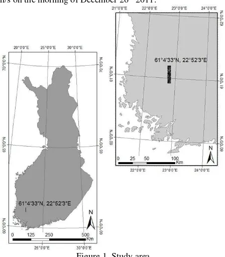
The study area is located in southwestern Finland with center coordinates 61°4 33 N, 22°52 3 E (Fig. 1) and covers approximately 173 km2. The area comprises mainly managed boreal forests and agricultural fields. The main tree species were Scots pine (Pinus sylvestris, L.), Norway spruce [Picea abies
(L.) H. Karst], and Silver and Downy birches (Betula spp.). The area is relatively flat with a terrain height range of approximately 50 to 111 m above sea level (asl) (deviation 12 m). On 26th and 27th of December 2011, the area was subjected to heavy winter storm called, which was the strongest storm in Finland in a decade (Finnish Meteorological Institute 2011). The storm caused extensive damage to the forest in the study area with the most damaging west and northwest winds blowing at an average speed of 18,3 m/s and a maximum speed of 28,7 m/s on the morning of December 26th 2011.
Figure 1. Study area.
2.2 LiDAR data
As the before-storm information open-access LiDAR data, obtained from the National Land Survey of Finland (NLS), were used. The NLS provides the data openly and freely for public use. According to the metadata afforded by the NLS the flying altitude of airborne LiDAR was 2,000 m, a maximum scan angle was ±20° and size of a footprint was 50 cm. Since DTM generation is the main use of these data the aforementioned specifications are used to optimize laser penetration to the forest floor, thus preferential collection times is during a bare-ground season or during spring time, when the trees have small leaves. The minimum point density of the NLS LiDAR data is 0,5 point/m2 and the elevation accuracy of the points in well-defined surfaces is 15 cm with a horizontal accuracy of 60 cm. The LiDAR data used in this study were
collected in 2008 during the spring. In the point clouds, the ground returns were already classified by the NLS by using the standard procedure developed by Axelson (2000). LasTools software (Isenburg, 2013) was used to merge the map sheets of NLS LiDAR data that covered the study area and to make a digital terrain model (DTM) and a digital surface model (DSM) of the point cloud with 1 m grid spacing.
2.3 Aerial images
Aerial imagery was acquired by Blom Kartta Oy © (Helsinki, Finland) on 8th of January 2012 to document the event of wind damage. The images were acquired using a Microsoft UltraCamXp (Microsoft UltraCam 2013), large-format mapping camera. The average flying height was 5,370 m above ground level (AGL) provided a ground sample distance (GSD) of 32 cm. The images were collected in a block structure, with 16 image strips and approximately 30 images per strip; the forward overlaps were 65%, and the side overlaps were 30%; the distances of the image strips were approximately 3,900 m. The atmosphere was clear, and the solar elevation was as low as 5°– 7°. The data were collected between 11:56 am and 14:11 pm local time (UTC +2). Before the aerial images were collected, the first snow had fallen, so that there was approximately 10–20 cm snow cover on ground. It is likely that there was also some snow on trees, but visual evaluation on images indicated that it was not significant (there is no ground truth data about this). These were very unusual and extreme conditions for a photogrammetric mapping project. Photogrammetric processing of used panchromatic images is explained in more detail in Honkavaara et al. (2013).
3. METHODS 3.1 Sample selection
Damaged areas needed to be mapped before it was possible to use spatial modelling in wind damage probability. The study area was and remote sensing data sets were the same that were used in Honkavaara et al. (2013). Honkavaara et al. (2013) developed and evaluated a method based on pre-storm LiDAR CHM and post-storm aerial imagery-derived CHM (normalized with LiDAR-based DTM) to detect wind damage. With that approach they were able to map wind-damaged forest stands with an accuracy of 100% for damaged and undamaged areas, 52% for minor damage, and 36% for low damage. We used this automated damage detection as stratification for our sample selection to obtain approximately equal samples in damaged and undamaged forest areas. A systematic grid (16 m x 16 m) was placed over the study area and 500 sample grid cells (i.e. sample plots) were selected across the study area (250 in each of the damaged and undamaged strata). Then, the damage-no damage-classification of each sampled grid cell was verified visually from the orthorectified aerial imagery acquired in January 2012. A sample plot was determined as damaged if there were a group of damaged trees (i.e. one fallen tree was not enough). During the visual inspection, 70 sample plots were removed because they were located in somewhere else than in forest (i.e. on an agricultural field, a road) or they were adjunct to field, road, a house, or other infrastructure. After visual inspection there were 430 sample plots for further analysis; 196 were classified as damaged and 234 as undamaged.
3.2 Predictor variable extraction
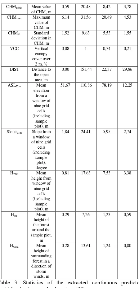
A 1 m resolution CHM was generated by subtracting DTM from DSM. Predictor variables for spatial modeling of PDAM were extracted from the LiDAR data (Appendix) for the sample plots (16m x 16m). Mean elevation above sea level (ASL), slope, and mean value of CHM were extracted for each plot and for a window of nine 16m x 16m grid cells (including the sample plot). Aspect was calculated as a categorical variable (i.e. northeast, southeast, southwest, and northwest) in order to capture the effects of direction of the damaging winds, namely northeast. Other predictors were mainly extracted for the sample plots and some also to their respective eight grid-cell-buffer areas (see Appendix for the explanations).
An estimate for forest vertical canopy cover (VCC) was computed by including all the points that were higher than 2 meters (CHM > 2m), which is commonly used threshold value for vegetation points (White et al. 2013). Open areas were extracted from the CHM where there were no canopy cover (defined using VCC) and contiguous area was larger than 1 ha. Although there may have been some low vegetation in areas where CHM was less than 2 m, it was presumed that wind can also cause damages to sites adjunct to low vegetation (often elevation, slope, tree species, and height of trees). The discrete nature of the dependent variable in our study (i.e., damage, no damage) was well suited to the use of LR. It has been applied widely in forestry to estimate tree and stand survival under competition (e.g., Monserud, 1976; Vanclay, 1995; Monserud & Sterba, 1999; Shen et al. 2000; Yao et al. 2001; Vastaranta et al. 2012) but also snow and wind damages (Valinger & Fridman, 1997; Canham et al. 2001; Scott & Mitchell, 2005; Vastaranta et al. 2011). In the field of remote sensing, logistic regression has been used for land cover change detection (e.g., Fraser et al. 2003; Fraser et al. 2005), modelling the impact of insect damage (Lambert et al. 1995; Ardö et al. 1997; Magnussen et al. 2004; Fraser & Latifovic, 2005; Wulder et al. 2006), but also in mapping the risk of fire severity (Montealegre et al. 2014).
In logistic regression the probability of an even to occur is the dependent variable which is transformed into a logit variable to make linearize the relationship between the response variable (i.e. probability) and the explanatory variables. The logit variable is calculated here as the neperian logarithm (ln) of the ration of the probability of success (p) over the probability of
where ln = the neperian logarithm
p the probability of success (i.e., damaged)
β0, β1, βn = regression parameters
x1, xn = the variables explaining the probability
The predictor variables (xi) it can be either continuous or discrete and randomly distributed or not.
Logistic regression is not subjected to many of the restrictive assumptions of ordinary least squares regression (OLS) (i.e. normal distribution of the dependent variable and error terms, homogeneity of variance, interval or unbounded independent variables) (Press & Wilson, 1978; Rice, 1994) because logistic regression calculates changes in the logit variable, not in the dependent variable itself (Hosmer & Lemeshow, 2000). However, when applying the estimated LR model to predict wind damage probabilities (PDAM) for the study area, the predicted probabilities were calculated by transforming them back to their original scale (Eq. 2):
exponentiating the coefficients. Exponentiated coefficients (eβ0, eβ1, etc.) can be interpreted as change of the odds of the event of interest (wind damage) to happen when that specific predictor variable changes one unit and other variables are hold at a fixed value. The signs of the coefficients (β0, β1, etc.) indicate if the ratio-change in the odds of wind damage is increasing or decreasing. To further interpret the exponentiated coefficients we calculated the percentage change in the odds (Eq. 3).
e
1
*
100
(3)3.4 Predictor variable selection
Potential predictor variables were tested using logistic regression analysis in R (v. 3.1.1, R Development Core Team, 2007). Predictors of wind damage were selected based on previous studies (Peltola et al. 1999; Jalkanen & Mattila, 2000; Hanewinkel et al. 2008), by analyzing the sample plot data, correlations, and on preliminary modelling results. Thus, the predictor variables were chosen on the basis of biological plausibility as well as statistical significance. Preliminary models were also compared using Akaike’s information criterion, AIC (Eq. 4):
2
log
L
2
k
AIC
(4)where L= maximum likelihood function for a model
k = number of independently adjusted parameters within the model
AIC is a measure of relative quality of a model, thus it estimates relative information loss by using certain model and it can be used in selecting a model from a set of models by selecting a model with minimum AIC value (Akaike, 1974).
After the selection of preliminary predictor variables, final predictors were selected using stepwise logistic regression with both forward and backward selections. The maximum number of steps to be considered was 1000.
3.4 Model validation and mapping
When verifying the significance that each predictor variable had for the model, we used Wald z-statistics (Hosmer & Lemeshow 2000) and their associated p-values. In other words, the Wald test works by testing a null hypothesis where one or several parameter of interest is equal to zero, i.e. removing them from the model will not substantially affect the prediction results. A predictor variable with a small coefficient relative to its standard error would not improve the prediction of the dependent variable (Stata FAQ 2014). When selecting the predictor variables we decided the statistical significance of p-values of Wald z-statistics needed to be at a maximum of 0.01 for the predictors in order to be sufficiently strong. Overall prediction accuracy was also used when comparing different combinations of predictor variables. A Likelihood Ratio Test (LRT) was used to measure how well our model fits (i.e., the called a risk map. The risk map allowed us to identify the areas of high risk across the study area. In risk map the employed cell size (16 m x 16 m) was the same that was used when sample cells (plots) were selected. If the predicted risk probability was over 0.5, it was interpreted as damage. Accuracy of risk map was evaluated by comparing it to the reference obtained by visual interpretation of aerial images. Two-scheme classification accuracy percentage and Cohen’s kappa value (Cohen 1960; Gramer et al. 2014) were calculated for the risk map (Eq. 5).
where Pr(a) = the overall agreement among raters
Pr(e) = the expected chance agreement (if agreement occurs by chance only)
If the raters are in complete agreement then K = 1. If there is no agreement among the raters other than what would be expected by chance (as defined by Pr(e)), K = 0.
4. RESULTS
4.1 Factors explaining the event of wind damage
Variables describing forest structure were calculated from CHM. CHMmean and CHMmax can be expected to explain stand maturity and they were higher in damaged plots (means: 9,7 m vs. 7,3 m and maximum values: 21,3 m vs. 19,8 m), thus it can be expected that the damaged plots were more mature. Most of the sample plots (86,7 %) were located inside forest stands and based on our analyses there were no trend that plots adjunct to an open area would be more vulnerable to wind damage. bigger (9,1 m) than of undamaged plots (6,2 m).
Topography-related variables derived from the DTM indicated that undamaged sample plots were in slightly steeper slopes (undamaged 6,3° vs. damaged 5,5°). Local topography variation (DTMsd) was slightly larger in undamaged areas (0.37 m vs. 0.33 m). On average damaged sample plots located five meters higher elevation (asl) (81,0 m) than the undamaged plots (76,0 m).
4.2 Selection of predictor variables and mapping the winda damage probability
The highest correlations (r=0,99) were found between DTMmean and DTMmax as well as DTMmean and ASL27m. CHMmean, on the other hand, was highly correlated with H27m (r=0,85) and with CHMmax (r=0,57). For other pairs of LiDAR-derived variables the correlations were low (r<0,5). After investigating correlations between different predictor variables, the predictor variables that were not highly (r>0,5) correlated or depended with each other were entered to the automatic stepwise selection of predictors. There were various combinations with the LiDAR-derived predictor variables to enter the selection of predictors.
Closeness to an open area was assumed to be significant predictor variable for the model; however, because the majority of sample plots were located inside forest stands, in our data the closeness variable was not a significant predictor when entered to the model. On average, the sample plots had taller trees than their surrounding forest in the direction where the storm winds came (west and northwest). This resulted with a decrease in the modelled damage probability, and since it was not statistically significant to the model, predictor describing the mean height of the tree in west and northwest (Hwind) was not included in the final model.
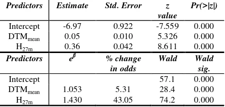
Mean height around the sample plots (plot area included) gave better results than mean height only within the sample plots, prediction accuracy with Kappa value of 0,47 and chi-square of likelihood ratio test (LRT) 209,70 with respective p-value less than 0,0001.
Predictors Estimate Std. Error z
value
Table 2. Parameters and fit statistics for the logistic regression model with mean elevation (DTMmean) and mean height around
sample plots (H27m) as predictor variables.
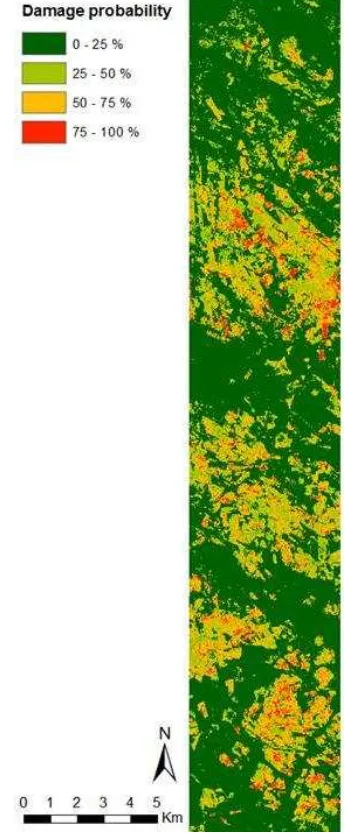
LR model was used to estimate the probability of wind damage for the entire study area. Model output was a continuous probability surface or risk map (Figure 3), whereby the probability for wind damage is interpreted as risk (e.g. areas The International Archives of the Photogrammetry, Remote Sensing and Spatial Information Sciences, Volume XL-3/W2, 2015
with a high probability of wind damage can be described as high risk areas).
Figure 3. Risk map produced by calculating wind damage probability to the entire study area (cell size is 16 m x 16 m).
5. DISCUSSION
The main aim of this research was to investigate the applicability of open access LiDAR data for modelling and mapping the probability of wind damage at a 256m2 resolution in our study area in southern Finland. The spatial resolution was selected to be the same that is applied in LiDAR-based operational forest-management-planning inventory in Finland. Wind damage events have increased in recent years and there is a need to identify areas of high risk in order to include alternative management actions into forest management planning but also to respond to information needs in other sectors (e.g., electricity providers).
A logistic regression approach was used to model the wind damage probability (i.e. wind damage risk) because it has been widely applied in the modeling of forest disturbances (Valinger & Fridman 1997; Fraser & Latifovis 2005; Wulder et al. 2006; Hanewinkel et al. 2008; Vastaranta et al. 2012). The damaged
plots were located at higher elevations and mean canopy height was higher in damaged plots than in undamaged plots. In our analyses, the most important spatial factors explaining the probability of wind damage (PDAM) were DTMmean and H27m. The predictor H27m described the mean value of CHM from a window of nine 16 m x 16 m grid cells, including the sample plot, and it provided more predicative power than mean height within a sample plot (CHMmean). As expected, these two variables (DTMmean and H27m) describing local topography and canopy height can provide valuable information on the damage probability (i.e. risk) in a robust way. This is also supported by previous research (Valinger & Fridman, 1997; Peltola et al. 1999; Jalkanen & Mattila 2000; Hanewinkel et al. 2008) where wind damage risk factors were studied with extensive sample plot data sets without risk mapping.
Surface models such as DTM and CHM are more robust for different flight and scanning parameters than 3D LiDAR point metrics that are generally used in area-based forest inventory (e.g. Næsset 2002; White et al. 2013). Because we wanted to have a robust model without a need for campaign-to-campaign or sensor-to-sensor calibration which is required when 3D point metrics are used, the LiDAR 3D point metrics were not used in the modelling. In addition, LiDAR surface models, such as DTM and DSM are usually readily available products that a user can order without a need of further knowledge about LiDAR processing.
The mean height of adjunct forest in the source wind direction of the sample plots was considered to offer shelter effect for the sample plots. However, on average the mean height of the damaged plots was higher than the mean height of the assumed shelter forest in northwest where the most destructive winds were blowing in our study area. Thus, the risk of wind damage decreased as the mean height of forest in the source wind direction increased which provided evidence about the shelter effect of the adjunct forest in northwest.
The study area is relatively flat where terrain heights do not vary significantly (standard deviation of DTM at the sample plots was 12 m) which we assumed to be the reason for the fact that slope and aspect were not significant factors in explaining the wind damage probability in the modelling. Another variable that was expected to have an effect on PDAM but in the end was not significant in our study was the distance to open area (Close). This may be due to the unique configuration of open and forest areas in our study site and merits further investigation (e.g. how much the unfrozen ground had an impact at the time when the damage occurred).
We used the output from the logistic regression, that was a probability of damage occurring, to produce a risk map describing the likelihood that any given grid cell has wind damage. We gained 73 % prediction accuracy with the logistic regression model compared to visual interpretation when predicting the probability of damage or no damage. This means that if similar storm would happen in similar conditions (such as temperature, soil moisture, wind direction etc.) we would be able to map the risk of the damage with high accuracy. In practice, much lower accuracies will be obtained due to variation in many natural factors.
6. CONCLUSIONS
The results of this study substantiated the applicability of open-source remote sensing data to map wind damage probability (PDAM). One implication is the generation of a continuous probability surface to represent the risk of wind damage. This probability surface was presented in this study as a risk map of wind damage. This risk map provides forest managers, owners, and authorities as well as electricity companies with much needed information for planning. Moreover, our results show that the LiDAR data, which are spatially extensive and increasingly openly accessible, can be used alone to estimate PDAM with acceptable levels of accuracy if detailed forest resource information is unavailable or outdated.
Use of the freely and openly accessible LiDAR data for estimating the risk of wind damage, as demonstrated herein, provides an example of additional beneficial uses for these data sets. Increasing the value of the open-access data is one of the objectives in collecting detailed forest resource information in Finland and this study serves that purpose.
ACKNOWLEDGEMENTS
The authors are grateful to Blom Kartta Oy for their support in providing the image materials for this study and to the National Land Survey of Finland for the laser scanning data. This study was supported by the financial aid from the Academy of Finland in the form of the Centre of Excellence in Laser Scanning Research (CoE-LaSR) 272195 as well as the Ministry of Agriculture and Forestry (LuhaGeoIT) DNro. 350/311/2012. Kimmo Nurminen is thanked for his assistance with image processing and selecting sample plots from the study area.
REFERENCES
Aggett, G.R. and Wilson, J.P., 2009. Creating and coupling a high-resolution DTM with a 1-D hydraulic model in a GIS for scenario-based assessment of avulsion hazard in a gravel-bed river. Geomorphology, 113(1-2), pp. 21–34.
Akaike, H. 1974. A new look at the statistical model identification. IEEE Trans Automat Contr, 19(6), pp. 16–723. doi:10.1109/TAC.1974.1100705.
Ardö, J., Pilesjö, P., and Skidmore, A., 1997. Neural networks, multitemporal Landsat Thematic Mapper data and topographic data to classify forest damages in the Czech Republic. Can J Remote Sens, 23(3), pp. 217– 229.
Axelsson, P., 2000. DEM generation from laser scanner data using adaptive TIN models. International Archives of Photogrammetry and Remote Sensing. 33(B4/1), pp. 110-117.
Canham, C.D., Papaik, M.J., and Latty, E.F., 2001. Interspecific variation in susceptibility to windthrow as a function of tree size and storm severity for northern temperate tree species. Can. J. For. Res, 31(1), pp. 1–10.
Fraser, R.H. and Latifovic, R., 2005. Mapping insect-induced tree defoliation and mortality using coarse spatial resolution satellite imagery. Int J Remote Sens, 26(1), pp. 193–200.
Fraser, R.H., Abuelgasim, T.A., and Latifovic, R., 2005. A method for detecting large-scale forest cover change using coarse spatial resolution imagery. Remote Sens Environ, 95(4), pp. 414-427.
Fraser, R.H., Fernandes, R., and Latifovic, R., 2003. Multi-temporal mapping of burned forest over Canada using satellite-based change metrics. Geocarto Int, 18(2), pp. 37–47.
Gueudet, P., Wells, G., Maidment, DR., and Neuenschwander, A., 2004. Influence of the post-spacing density of the LiDAR-derived DEM on flood modeling. In : Proceedings of the 2004 American Water REsources Association Spring Specialty Conference. Nashville, Tennessee.
Hanewinkel, M., Breidenbach, J., Neeff, T., and Kublin, E., 2008. Seventy-seven years of natural disturbances in a mountain forest area – the influence of storm, snow, and insect damage analyzed with a long-term time series. Can. J. For. Res, 38(8), pp. 2249-2261.
Heino, E. and Pouttu, A., 2013. Metsätuhot vuonna 2012. [Forest damages in 2012]. Finnish. Working Papers of the Finnish Forest Institute 269.
Hohenthal, J., Alho, P., Hyyppä, J., and Hyyppä, H., 2011. Laser scanning applications in fluvial studies. Prog Phys Geogr, 35, pp. 782-809. doi:10.1177/0309133311414605
Honkavaara, E., Litkey, P., and Nurminen, K., 2013. Automatic Storm Damage Detection in Forests Using High-Altitude Photogrammetric Imagery. Remote Sens, 5(3), pp. 1405-1424.
Hopkinson, C., Chasmer, L., and Hall, RJ., 2008. The uncertainty in conifer plantation growth prediction from multi-temporal lidar datasets. Remote Sens Environ, 112, pp. 1168– 1180.
Hosmer, D.W. and Lemeshow, S., 2000. Applied logistic regression. New York: John Wiley & Sons, Inc.
Härkönen, S., 2012. Estimating forest growth and carbon balance based on climatesensitive forest growth model and remote sensing data [dissertation]. Dissertationes Forestales
138. 56 p. Available from :
http://www.metla.fi/dissertationes/df138.htm.
Isenburg, M., 2013. LAStools—Efficient Tools for LiDAR Processing; Version 120628. [cited 2013 Mar 5]. Available from: http://lastools.org.
Jalkanen, A. and Mattila, U., 2000. Logistic regression models for wind and snow damage in northern Finland based on the National Forest Inventory data. For. Ecol. Manage, 135, pp. 315–330.
Lambert, N.J., Ardö, J., Rock, B.N., and Vogelmann, J.E., 1995. Spectral Characterization and regression based classification of forest damage in Norway spruce Stands in the Czech Republic using Landsat TM data. Int J Remote Sens. 16, pp. 1261– 1287.
Liao, Z., Hong, Y., Adler, R., and Bach, D., 2010. A physically based SLIDE model for landslide hazard assessments using remotely sensed data sets. In: Jiang, M., Liu, F., & Bolton, M. The International Archives of the Photogrammetry, Remote Sensing and Spatial Information Sciences, Volume XL-3/W2, 2015
Geomechanics and Geotechnics : From Micro to Macro. London: Taylor & Francis; pp. 807-813.
Lohmander, P. and Helles, F., 1987. Windthrow probability as a function of stand characteristics and shelter. Scand J For Res, 2, pp. 227–238.
Magnussen, S., Boudewyn, P., and Alfaro, R., 2004. Spatial prediction of the onset of spruce budworm defoliation. The Forestry Chronicle, 80, pp. 485–494.
Monserud, R.A., 1976. Simulation of forest mortality. Forest Science, 22, pp. 438– 444.
Monserud, R.A. and Sterba, H., 1999. Modeling individual tree mortality for Austrian forest species. For. Ecol. Manage, 113, pp. 109– 123.
Montealegre, A.L., Lamelas, M.T., Tanase, M.A., and de la Riva, J., 2014. Forest fire severity assessment using ALS in a Mediterranean environment. Remote Sens, 6, pp. 4240-4265. doi:10.3390/rs6054240.
Nagelkerke, N., 1991. A note on a general definition of the coefficient of determination. Biometrika, 78, pp. 691-692.
Næsset E., 2002. Predicting forest stand characteristics with airborne scanning laser using a practical two-stage procedure and field data. Remote Sens Environ, 81, pp. 88–99.
Næsset, E. and Gobakken, T., 2005. Estimating forest growth using canopy metrics derived from airborne laser scanner data.
Remote Sens Environ, 96, pp. 453–465.
Peltola, H., Kellomäki, S., Väisänen, H., and Ikonen, VP., 1999. A mechanistic model for assessing the risk of wind and snow damage to single trees and stands of Scots pine, Norway spruce, and birch. Can. J. For. Res, 29, pp. 647–661.
Press, S.J. and Wilson, S., 1978. Choosing between logistic regression and discriminant analysis. Am Stat, 73, pp. 699– 705.
R Development Core Team., 2007. R: A language and environment for statistical computing. R Foundation for Statistical Computing, Vienna, Austria. [cited 2011 Jun 27]. Available from: www.R-project.org.
Rice, J.C., 1994. Logistic regression: An introduction. In: Thompson, B., (editor) Advances in social science methodology. 3. Greenwich: CT’ JAI Press. pp. 191–245.
Scott, R.E. and Mitchell, S.J., 2005. Empirical modelling of windthrow risk in partially harvested stands using tree, neighbourhood and stand attributes. For Ecol Manage, 218, pp. 193-209.
Shen, G., Moore, J.A., and Hatch, C.R., 2000. The effect of nitrogen fertilization, rock type, and habitat type on individual tree mortality. For Sci, 47, pp. 203–213.
Stata FAQ: How can I preform the likelihood ration, Wald, and Lagrange multiplier (score) test in Stata [Internet]. UCLA: Statistical Consulting Group; [cited 2014 Nov 13]. Available from: http://www.ats.ucla.edu/stat/stata/faq/nested_tests.htm.
Valinger, E. and Fridman, J., 1997. Modelling probability of snow and wind damage in Scots pine stands using tree characteristics. For. Ecol. Manage, 97(3), pp. 215-222.
Vanclay, J.K., 1995. Growth models for tropical forests: a synthesis of models and methods. For Sci, 41, pp. 7 –42.
Vastaranta, M., Korpela, I., Uotila, A., Hovi, A., and Holopainen, M., 2011. Area-based snow damage classification of forest canopies using bi-temporal lidar data. In : Lichti, D. & Habib, A., editors. LaserScanning 2011 proceedings, pp 5.
Vastaranta, M., Korpela, I., Uotila, A., Hovi, A., and Holopainen, M., 2012. Mapping of snow-damaged trees in bi-temporal airborne LiDAR data. Eur J For Res, 131(4), pp. 1217-1228. DOI: 10.1007/s10342-011-0593-2.
White, J.C., Wulder, M.A., Varhola, A., Vastaranta, M., Coops, N.C., Cook, B.D., Pitt, D., and Woods, M., 2013. A best practices guide for generating forest inventory attributes from airborne laser scanning data using an area-based approach.
Forestry Chronicle, 89(6), pp. 722-723.
Wright, JA. and Quine, CP., 1993. The use of a Geographical Information System to investigate storm damage to trees at Wykeham Forest North Yorkshire. Scottish Forestry, 47(4), pp. 166–174.
Wulder, M.A., White, J.C., Bentz, B., Alvarez, M.F., and Coops, N.C., 2006. Estimating the probability of mountain pine beetle red-attack damage. Remote Sens Environ, 101, pp. 150-166.
Yao, X., Titus, S., and MacDonald, S.E. 2001., A generalized logistic model of individual tree mortality for aspen, white spruce, and lodgepole pine in Alberta mixedwood forests. Can. J. For. Res, 31, pp. 283– 291.
Yu, X., Hyyppä, J., Kaartinen, H., and Maltamo, M., 2004. Automatic detection of harvested trees and determination of forest growth using airborne laser scanning. Remote Sens Environ, 90, pp. 451–462.
APPENDIX
Predictor Description
Statistics within sample plots
Min Max Mean Sd
Slope Slope, degrees
1,57 30,18 5,94 3,46
Aspect Aspect, degrees
45,50 312,89 177,55 47,51
DTMmin Minimum value of DTM, m
49,36 109,91 77,51 12,26
DTMmean / ASL
Mean value of DTM / Elevation,
m
50,44 111,08 78,25 12,28
DTMmax Maximum value of DTM, m
51,91 112,14 79,06 12,34
DTMsd Standard deviation in elevation, m
0,06 2,68 0,35 0,32
CHMmin Minimum value of CHM, m
0,00 2,08 0,00 0,22
CHMmean Mean value of CHM, m
0,59 20,48 8,42 3,78
CHMmax Maximum value of CHM, m
6,14 31,56 20,49 4,53
CHMsd Standard deviation in
CHM, m
1,52 9,63 5,53 1,55
VCC Vertical canopy cover over
2 m, %
0,08 1 0,74 0,21
DIST Distance to the open
area, m
0,00 151,44 22,37 29,86
ASL27m Mean elevation
from a window of
nine grid cells (including
sample plot), m
51,67 110,86 78,19 12,25
Slope27m Slope from a window of nine grid
cells (including
sample plot), degree
1,84 24,41 5,95 2,74
H27m Mean
height from window of nine grid
cells (including
sample plot), m
0,81 17,63 7,53 3,38
Hsur Mean
height of the forest around the sample plot,
m
0,29 7,26 1,23 0,59
Hwind Mean height of surrounding
forest in a direction of
storm winds, m
0,28 13,61 1,24 0,80
Table 3. Statistics of the extracted continuous predictor variables for the sample plots (n = 430).
Predictor Description Distribution of classes Aspectpoint Aspect in
compass points
NE: 113 SE: 107 SW: 108 NW: 102 Close Closeness to
an open area
Next to an open area: 57 No next to an open area: 373
Table 4. Descriptions of extracted categorical predictor variables within sample plots (n=430).