ADAPTIVE PARAMETER ESTIMATION OF PERSON RECOGNITION MODEL
IN A STOCHASTIC HUMAN TRACKING PROCESS
W. Nakanishi a, * , T. Fuse a and T. Ishikawa a
a Dept. of Civil Engineering, The University of Tokyo, 7-3-1 Hongo, Bunkyo-ku, Tokyo 1138656 Japan - (nakanishi@civil, fuse@civil, ishikawa@trip).t.u-tokyo.ac.jp
KEY WORDS: State space modelling, Human tracking, Sequential image, Adaptive parameter estimation, Close Range
ABSTRACT:
This paper aims at an estimation of parameters of person recognition models using a sequential Bayesian filtering method. In many human tracking method, any parameters of models used for recognize the same person in successive frames are usually set in advance of human tracking process. In real situation these parameters may change according to situation of observation and difficulty level of human position prediction. Thus in this paper we formulate an adaptive parameter estimation using general state space model. Firstly we explain the way to formulate human tracking in general state space model with their components. Then referring to previous researches, we use Bhattacharyya coefficient to formulate observation model of general state space model, which is corresponding to person recognition model. The observation model in this paper is a function of Bhattacharyya coefficient with one unknown parameter. At last we sequentially estimate this parameter in real dataset with some settings. Results showed that sequential parameter estimation was succeeded and were consistent with observation situations such as occlusions.
1. INTRODUCTION
Human tracking method is classified into two manners. One is that in each frame human candidates are detected and then the same person is identified in adjacent frames. The other is that, in each frame, each human position is predicted from that of previous frame and then accurate position is calculated by a stochastic model using observed information. As we can consider pedestrian behaviour model for successive frames, this method has an advantage to tracking many persons simultaneously in complex situations in which occlusions and proximities are occurred (e.g. Ali and Dailey, 2009; Nakanishi and Fuse, 2012). Mathematically this method should be solved as a stochastic process. Typical formulation for this method is based on Bayesian statistics; predicted position is described by prior distribution, observed information corresponds to data and accurate position to posterior. When we use this method, we should define a likelihood function that describes likelihood of observed information occurred by given predicted position. We
call this likelihood function “observation model” in human
tracking method (explained later in detail). This paper aims at an estimation of parameters of observation model, that is, person recognition model, using a sequential Bayesian filtering method. We especially deal with a stochastic process for human tracking mentioned above.
A main problem on human tracking from sequential images is to identify the same person in successive frames. When we acquire colour information from an image, we use a human detection model to detect and then identify a person in adjacent frames. Any models used here have some parameters that correspond to sensitivity and thresholds. Usually this parameters are set empirically or adjusted to data in advance of tracking process. This means that we have to set models and parameters according to observations every time. We cannot directly apply a setting on one observation site to another. Moreover, we might have to change model settings on the same observation site on different time or day.
Thus in this paper we apply sequential Bayesian filtering to an estimation of this parameters and update parameters according to observations at each frame. We call this updating as an adaptive estimation. In addition to an advantage that parameters are automatically adjusted to change in observation situations as mentioned above, this adaptive estimation can deal with differences in prediction accuracy in a tracking process. When we use stochastic process like general state space model for tracking, an estimated human position is determined by both prediction by previous human position and detection by present observation. Therefore if prediction is quite accurate, then sensitivity of detection can be high; Sensitivity parameters can be set large, or thresholds parameters can be set high. In contrast, if prediction is uncertain, then detection sensitivity should be low.
In previous research (Nakanishi and Fuse, 2012) we assume a tracking process as a data assimilation process and describe it in a form of general state space model. Human position and size are defined as unobservable variables: state vectors, and stochastic pedestrian behaviour model is introduced into a system model. We assume that state vectors generate colour images according to a person recognition model: an observation model. We applied Bhattacharyya coefficient (Bhattacharyya, 1943) to formulate an observation model. While even we use only Bhattacharyya coefficient to formulate an observation model, we have slight knowledge about function forms and parameter settings that bring good observation models. Although experimental tests have been conducted in some function forms and parameters (Nakanishi and Fuse, 2014), parameters are decided in advance there.
In this paper we sequentially estimate a parameter of some observation models using general state space model. From this estimation we consider good parameters correspond to prediction and observation situations; how parameters should be according to prediction and observation accuracy.
2. MODELLING FRAMEWORK observation model p(zt|xt) is also a conditional density function
that represents a likelihood of realisation of zt given xt. After we the estimation result at time t-1.
If we need the estimated value for xt, following values are
(b) Posterior mode: Maximum a posteriori
1:
frequency of posterior equals to n percent
|
1:
Figure 1. General state space model
We use particle filter (Gordon, et al., 1993; Kitagawa, 1996) for calculating equation (1), for some models are assumed to be non-linear. In this work we use 65536 particles to approximate posteriors. We also use Halton sequences (Halton, 1964) to generate prior (predictive) distributions. They are typical quasi-random number sequences. Thus good approximation of posteriors with less number of particles is expected.
2.2 Self-Organizing Modelling
Now we consider that a set of parameters θ of observation model is also unobservable. This means that parameters of a person recognition model can take different value from time to time. We introduce θ into state vector as follows (Kitagawa,
Then we can describe system and observation models as follows.
1
is random walk model. Then we can calculate a posterior in the same way as equation (1),Marginal distributions are calculated as
t|
1:t
t|
1:t
tp
x z
p
x z
d
θ
(9)
t|
1:t
t|
1:t
tp
θ
z
p
x z
d
x
(10)We obtain this posteriors at each time instant t; Equation (9) is estimated positions and (10) is estimated parameters at each time. These are the estimated results in this paper.
3. MODEL SETTINGS
3.1 State Vector and Observation Vector
We use “BEHAVE” dataset (Blunsden and Fisher, 2010; Figure
2) for analyses. This dataset provides sequential images and ground truth of human positions and sizes of rectangles on these images. We define four-dimensional xt, representing human
position and its size, considering an inscribed ellipse in the rectangle (equation (11)). We also define zt as colour values at
each pixel inside the ellipsoid (equation (12)). We define state and observation vectors at one second intervals. This means that we predict each second human position of one second after. And we also use colour information from images every one second.
x y a a
, ,
x,
y
T
x
(11)
,
,
T xy
r
xyg
xyb
xyz
(12)where x, y = coordinates of each pixel on images
ax, ay = ellipse’s semidiameter of x and y
respectively
rxy, gxy, bxy = corresponding colour value at pixel (x, y)
Figure 2. Example of used dataset (Blunsden and Fisher, 2010)
3.2 System Model
System model in this paper describe a difference of positions and sizes of the same person in successive frames. We consider only changes in positions and assume that sizes are predicted precisely at each frame. Then we set system model in two manners. One is that we set it as difference of true values. This means that relative value of position change is precisely predicted. The other is that we set it with error terms in addition to relative position changes. Details are explained later.
3.3 Observation Model
We build a model of p(zt|xt) as follows, using Bhattacharyya
coefficient B and a parameter c (Figure 3):
, ,
i i i r g b
B
p q
(13)
|
m mm
p f B f p q
z x (14)
, c
1
cB c
ce
f B
e
(0<c) (15)where B = Bhattacharyya coefficient
i = pixel value
r, g, b = corresponding colour
p, q = normalized histogram of previous and predictive position respectively
pm = relative frequency of pixel value m in histogram p
As shown in equation (13), the domain of Bhattacharyya coefficient is [0, 1]. Here an integration of equation (15) with interval [0, 1] is one for any B and c. This fact theoretically guarantee that adaptive estimation can be done. This parameter
c corresponds to θ in Chapter 2 in following part of this paper.
Figure 3. Observation model with parameter B and c
4. EXPERIMENTAL RESULTS
4.1 Settings
We conduct experiments on dataset mentioned above in five settings shown in Table 4.
Firstly we set initial state vectors as a true value from the dataset and system models as a true model: the difference between true values of successive frames. We set several patterns for the parameter’s initial value and system models of that parameter. These are setting 1-3. Initial value of c in setting 1 and 2 are decided as the maximum likelihood estimator that is calculated using dataset itself. In contrast, that of setting 3 is smaller value. The difference between setting 1 and 2 is variance of system model of c; in setting 2 system model of c has large variance than that of setting 1.
Secondly we change system models and initial values of human position. These are setting 4 and 5. This is natural assumptions; the former setting is corresponding to uncertainty in prediction models, and the latter in detection models. This time we get not only the posterior of the parameter but also the posteriors of human position.
4.2 Results and Discussions
It is difficult to evaluate an accuracy of estimation of state vectors, for state vectors themselves cannot be observed. So in this paper we discuss results qualitatively. We take a result of one person as an example to explain and discuss about results. We confirmed that similar tendencies are common among other persons. Results are shown in Figure 5. Solid lines show posterior mean and dashed lines show 25, 50 and 75 percentiles respectively.
Table 4. Setting for analyses
Setting Initial value of c Initial error of position System model of c Noise of system model of position
1 8.52 0 ct~N(ct-1, 0.1) 0
2 8.52 0 ct~N(ct-1, 0.5) 0
3 2.00 0 ct~N(ct-1, 0.1) 0
4 2.00 0 ct~N(ct-1, 0.1) N(0, diag(25))
5 2.00 5 pix for x-y each ct~N(ct-1, 0.1) N(0, diag(25))
Setting 1 Setting 2 Setting 3
Setting 4 Setting 5
Solid lines show expected values of posteriors; Dashed lines show 25, 50 and 75 percentiles respectively;
t is frame number and framerate is 25 [fps]. Figure 5. Posterior distributions of parameter c in each setting
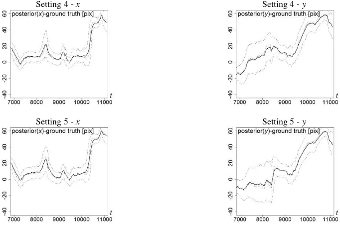
Setting 4 - x Setting 4 - y
Setting 5 - x Setting 5 - y
Solid lines show expected values of posteriors; Dashed lines show 25, 50 and 75 percentiles respectively;
t is frame number and framerate is 25 [fps]. Figure 6. Posterior distributions of positions in each setting
In setting 1-3, sequential Bayesian estimation are succeeded and posterior distributions are similar to each other. We also found that the value of parameter is low when a person is occluded by other person: around frame #8200 and #9200. This is the expected tendency, for Bhattacharyya coefficient is low when occlusions occur. This showed that adaptive parameter estimation was useful in that values of parameter changed according to observation situations.
In setting 4, when noise of system model is large, the accuracy of position estimation became low when there were occlusions. This is consistent with the results of setting 1-3 above. And after frame #10000 we found that the parameter value became slightly high. This is because once we lost an accurate position of a person, then we compared two histograms composed of background pixels. This fact is also shown from position’s marginal posteriors. Figure 6 shows posteriors of residual (relative value to ground truth). If shape of this distribution is sharp around zero, estimations are good. Actually from around frame #10000 we lost the accurate position in each coordinates
x and y. Especially y coordinates was difficult to predict precisely, for a little difference in y value cannot be affected to shape of colour histogram; clothes tended to be the same colour in upper and lower pixels of a certain pixel, and also background pixels be the same colour in upper and lower of a certain person. In setting 5, very similar tendency to setting 4 was shown.
In summary, the observation model in this paper can deal with prediction errors that are less than 10 pixels, otherwise it is difficult to correct errors and estimate precise positions of persons. In order to achieve successful tracking in such a case, parameter value should be kept low during low accuracy of prediction. Also it may bring about good result to introduce foreground detection model into proposed model and to use only foreground pixels to make histograms.
5. CONCLUSION
In this paper we estimated the parameter of person recognition model adaptive to observation data by using sequential Bayesian filtering. After formulate the estimation, we applied the proposed method to dataset. From results we showed that appropriate parameter changes from time to time according to the situation of observation and prediction. Also we discussed about the tendency of parameter change by comparing parameter values and some settings for parameter estimation. Basically the results were consistent with settings and situations. Thus we could confirm that sequential Bayesian filtering is a useful way to deal with time and space varying parameter estimation.
Future works are as follows. Firstly we conduct such analyses on other models. For example, we combine the models with foreground detection models to deal with larger prediction errors. Also we employ models with more than one parameter to deal with more complex situations. At last we try to find the way to formulate observation models themselves, not only their parameters, according to the dataset. To achieve such estimations with larger calculation amount, we have to consider how to approximate posteriors by smaller particles. An application of merging particle filter (Nakano et al., 2007) or Rao-Blackwellisation (Casella and Robert, 1996) is one possible way.
References:
Ali, I. and Dailey, M., 2009. Multiple human tracking in high-density crowds, Advanced Concepts for Intelligent Vision Systems, LNCS 5807, pp.540-549.
Bhattacharyya, A., 1943. On a Measure of Divergence between Two Statistical Populations Defined by Their Probability Distributions, Bulletin of the Calcutta Mathematical Society, 35(14), pp.99-109.
Blunsden, S. J. and Fisher, R. B., 2010. The BEHAVE Video Dataset: Ground Truthed Video for Multi-person Behavior Classification, Annals of the BMVA, 2010(4), pp.1-11.
Casella, B. Y. G. and Robert, C. P., 1996. Rao-Blackwellisation of Sampling Schemes, Biometrika, 83(1), pp.81-94.
Gordon, N. J., Salmond, D. J. and Smith, A. F. M., 1993. Novel Approach to Nonlinear / Non-Gaussian Bayesian State Estimation. Radar and Signal Processing, IEE Proceedings F, 140(2), pp.107-113.
Halton, J. H., 1964. Algorithm 247: Radical-inverse quasi-random point sequence, Communications of the ACM, 7(12), pp.701-702,
Jaynes, E. T., 2003. Probability Theory: The Logic of Science, Cambridge University Press, pp.172-175.
Kitagawa, G., 1996. Monte Carlo Filter and Smoother for Non-Gaussian Nonlinear State Space Models. Journal of Computational and Graphical Statistics, 5(1), pp.1-25. Kitagawa, G., 1998. A Self-Organizing State-Space Model,
Journal of the American Statistical Association, 93(443), pp.1203-1215.
Nakanishi, W. and Fuse, T., 2012. Multiple Human Tracking in Complex Situation by Data Assimilation with Pedestrian Behavior Model. ISPRS Archives, 39-B3, pp.409-414.
Nakanishi, W. and Fuse, T., 2014. Sensitive Analysis of Observation Model for Human Tracking Using a Stochastic Process, ISPRS Archives, 40-5, pp.445-450.
Nakano, S., Ueno, G. and Higuchi, T., 2007. Merging Particle Filter for Sequential Data Assimilation, Nonlinear Processes in Geophysics, 14(4), pp.395-408.