Full Terms & Conditions of access and use can be found at
http://www.tandfonline.com/action/journalInformation?journalCode=ubes20
Download by: [Universitas Maritim Raja Ali Haji] Date: 13 January 2016, At: 01:03
Journal of Business & Economic Statistics
ISSN: 0735-0015 (Print) 1537-2707 (Online) Journal homepage: http://www.tandfonline.com/loi/ubes20
The Shape of the Risk Premium
Oliver Linton & Benoit Perron
To cite this article: Oliver Linton & Benoit Perron (2003) The Shape of the Risk Premium,
Journal of Business & Economic Statistics, 21:3, 354-367, DOI: 10.1198/073500103288619052
To link to this article: http://dx.doi.org/10.1198/073500103288619052
Published online: 01 Jan 2012.
Submit your article to this journal
Article views: 60
The Shape of the Risk Premium: Evidence
From a Semiparametric Generalized
Autoregressive Conditional
Heteroscedasticity Model
Oliver L
INTONDepartment of Economics, London School of Economics, Houghton Street, London WC2A 2AE, U.K. (lintono@lse.ac.uk)
Benoit P
ERRONDépartement de Sciences Économiques, CIREQ, CIRANO, Université de Montréal, C.P. 6128, Succursale Centre-ville, Montréal, Québec H3C 3J7, Canada (benoit.perron@umontreal.ca)
We examine the relationship between the risk premium on the Center for Research on Security Prices (CRSP) value-weighted index total return and its conditional variance. We propose a new semiparametric model in which the conditional variance process is parametric and the conditional mean is an arbitrary function of the conditional variance. For monthly CRSP value-weighted excess returns, the relationship between the two moments that we uncover is nonlinear and nonmonotonic.
KEY WORDS: Asset pricing; Autoregressive conditional heteroscedasticity; Backtting; Fourier series; Kernel; Risk premium.
1. INTRODUCTION
Modern asset pricing theories, such as those of Abel (1987, 1999), Cox, Ingersoll, and Ross (1985), Merton (1973), and Gennotte and Marsh (1993), imply restrictions on the time se-ries properties of expected returns and conditional variances of market aggregates. These restrictions are generally quite complicated, depending on utility functions as well as on the driving process of the stochastic components of the model. However, in an inuential paper, Merton (1973) obtained very simple restrictions albeit under somewhat drastic assumptions. He showed in the context of a continuous-time partial equilib-rium model that
¹tDE[.rmt¡rft/jFt¡1]D°var[.rmt¡rft/jFt¡1]D° ¾t2; (1)
where rmt andrft are the returns on the market portfolio and
risk-free asset andFt¡1is the market-wide information avail-able at timet¡1. The constant° is the Arrow–Pratt measure of relative risk aversion.
The simplicity of the foregoing restrictions and their appar-ent congruence with the original capital asset pricing model (CAPM) restrictions (see Sharpe 1964; Lintner 1965) has mo-tivated a large number of empirical studies that test some vari-ant of this restriction. A convenient statistical framework for examining the relationship between the quantities¹t and¾t2
in discrete nancial time series is the autoregressive condi-tional heteroscedasticity (ARCH) class of models (see Boller-slev, Chou, and Kroner 1992; BollerBoller-slev, Engle, and Nelson 1994 for references). Engle, Lilien, and Robins (1987) ex-amined the relationship between government bonds of diffent maturities using the ARCH-M model in which the er-rors follow an ARCH.p/ process and ¹t D¹.¾t2/ for some
parametric function¹.¢/. They examined¹tD°0C°1¾t and
¹tD°0C°1ln.¾t2/and found that the latter specication
pro-vided the better t. French, Schwert, and Stambaugh (1987)
and Nelson (1991) also examined this relationship using gen-eralized autoregressive conditional heteroskedastic (GARCH) models.
Gennotte and Marsh (1993) argued that the linear relation-ship (1) should be regarded as a very special case. They con-structed a general equilibrium model of asset returns and de-rived the equilibrium relationship
¹tD° ¾t2Cg.¾
2
t/; (2)
where the form of g.¢/ depends on preferences and on the parameters of the distribution of asset returns. If the repre-sentative agent has logarithmic utility, theng.¢/´0, and the simple restrictions of Merton pertain. In addition, Backus, Gre-gory, and Zin (1989) and Backus and Gregory (1993) provided simulation evidence thatg.¢/, and hence¹.¢/, could be of arbi-trary functional form in general equilibrium. Whitelaw (2000) developed these empirical ndings into an equilibrium asset-pricing model with regime changes in which the relation is lin-ear within each regime but overall nonlinlin-ear due to the presence of the two distinct regimes. Veronesi (2001) also developed a model in which investors receive noisy signals in which the shape of the relation between the risk premium and the con-ditional variance is ambiguous and depends on investor uncer-tainty.
Pagan and Hong (1990) argued that the risk premium, ¹t,
and the conditionalvariance,¾t2, are highly nonlinear functions of the past whose form is not captured by standard paramet-ric GARCH-M models. They estimated¹tand¾t2
nonparamet-rically and found evidence of considerable nonlinearity. They
© 2003 American Statistical Association Journal of Business & Economic Statistics July 2003, Vol. 21, No. 3 DOI 10.1198/073500103288619052
354
then estimated±from the regression
rmt¡rftD¯0xtC±¾t2C´t; (3)
by the least squares and instrumental variables methods with
¾t2substituted for the nonparametric estimate, nding a nega-tive but insignicant±. Perron (2003) analysed this approach using weak instrument asymptotics and found similar re-sults.
The Pagan and Hong (1990) approach has a couple of draw-backs. First, the conditional moments are calculated using a restricted conditioning set—the information set used in den-ing ¹t and ¾t2 contained only a nite number of lags, that
is, Ft¡1 D fyt¡1; : : : ;yt¡pg for some xed p and data series ytDrmt¡rft. This greatly restricts the dynamics for the
vari-ance process. In particular, if the conditional varivari-ance is highly persistent, then the nonparametric estimator of the conditional variance provides a poor approximation, as conrmed by the simulation evidence reported by Perron (1998). Second, lin-earity of the relationship between¹t and¾t2 is imposed, and
this seems to be somewhat restrictive in view of earlier nd-ings.
In this article, we investigate the relationship between the risk premium and the conditional variance of excess returns on the Center for Research on Security Prices (CRSP) value-weighted index. We consider a semiparametric specication that differs from previous treatments. In particular, we choose a parametric form for the variance dynamics [in our case, ex-ponential GARCH (EGARCH)], while allowing the mean to be an unknown function of¾t2. This model takes into account the high level of persistence and leverage effect found in stock index return volatility, while at the same time allowing for an arbitrary functional form to describe the relationship between risk and return at the market level. We develop two estimation methods for this model: a Fourier series method and a method based on kernels. The kernel method is based on iterative one-dimensionalsmoothing and is similar in this respect to the back-tting method for estimating additive nonparametric regression (see Hastie and Tibshirani 1990). We also suggest a bootstrap algorithm for obtaining condence intervals. Using these meth-ods, we nd evidence of a nonlinear and nonmonotonic rela-tionship between the risk premium and the conditional vari-ance.
Other work applying nonparametric methods to this problem has been done by Boudoukh, Richardson, and Whitelaw (1997) and Harvey (2001). Our work differs from theirs in the para-metric specication that we choose for the conditionalvariance. This enables joint estimation of the two elements of interest, as described in Section 3.
In the next section we discuss the specication of our model, while in Sections 3 and 4 we describe how to obtain point and interval estimates respectively. In Section 5 we present our em-pirical results and the results of a small simulation experiment, and in Section 6 we conclude.
2. A SEMIPARAMETRIC-MEAN EXPONENTIAL GENERALIZED AUTOREGRESSIVE CONDITIONAL HETEROSCEDASTICITY MODEL
We suppose that the excess returnsytare generated as
ytD¹.¾t2/C"t¾t; tD1;2; : : : ;T; (4)
where "t is a martingale difference sequence with unit
(con-ditional) variance and ¹.¢/is a smooth function of unknown functional form. The restriction thatE[ytjFt¡1], whereFt¡1D
fyt¡jg1jD1, depends on the past through only¾t2 is quite severe
but is a consequence of asset pricing models (e.g., Backus and Gregory 1993; Gennotte and Marsh 1993). In any case, it is possible to generalize this formulation in a number of direc-tions. It is straightforward to incorporate xed explanatory vari-ables, lagged¾t2, or laggedyt either as linear regressors or
in-side the unknown function¹.¢/. More complicated dynamics for"t, such as an ARMA.p;q/model and a multivariate
exten-sion, can also be accommodated.
We propose using a parametric function for the conditional variance so as to allow for rich dynamics in the volatility. To be specic, we consider the EGARCH model introduced by Nel-son (1991),
The presence of the lagged dependentvariablesht¡jallows very
rich dynamics for the variance process itself, which cannot yet be achieved by nonparametric methods. The foregoing model also allows both the sign and the level of"t¡k to affect¾t2—
good news and bad news can have different effects on volatility, hence allowing the possibility of the so-called “leverage effect” in stock returns. The parameterd controls the relative impor-tance of the symmetric versus asymmetric effects. Evidence of such a leverage effect in returns on stock indices is widespread in the literature (e.g., Nelson 1991 for daily data and Braun, Nelson, and Sunier 1991 for monthly data).
A number of authors (e.g., Nelson 1991), have found that standardized residuals from estimated GARCH models are lep-tokurtic relative to the normal (see also Engle and Gonzalez-Rivera 1991). We thus assume that"t has a distribution within
the generalized error distribution (GED) family,
f."/Dºexp
where 0 is the gamma function. The GED family of errors includes the normal.ºD2/, uniform.ºD 1/, and Laplace
.ºD1/as special cases. The distribution is symmetric about 0 for allºand has nite second moments forº >1. With this den-sity, we obtain thatEj"tj D.¸21=º0.2=º//= 0.1=º/ (Hamilton
1994, p. 669).
We assume that the parameter values satisfy the requirements for stationarity given by Nelson (1991). Carrasco and Chen (2002) established a general result about the dependence prop-erties of a general class of volatility models, which suggests that the processytis¯mixing under some conditions.
Newey and Steigerwald (1997) showed that quasi-likelihood estimators in GARCH models based on distributions other than the normal are generally inconsistent. Therefore, we also inves-tigate our EGARCH.p;q/specication for the variance com-bined with a normal error distribution.
The main difference between our model and previous treat-ments is that we do not restrict the functional form of ¹.¢/a priori. This has a number of implications for both estimation and testing. In particular, a simple consistent estimator of¹.¢/
is difcult to obtain and would appear to depend on rst ob-taining consistent estimates of the parameters of the variance process. On the other hand, to estimate these parameters, we need to have a good estimate of ¹.¢/. In the next section we propose a solution to this problem.
3. ESTIMATION
3.1 Parametric Estimation
Estimation of the unknown parameters by maximum likeli-hood when ¹.¢/ is known apart from a nite number of pa-rameters, say ¿, has been considered by Engle et al. (1987) and Nelson (1991). In this case let µ D.Á; ¿ /, where ÁD .a;b1; : : : ;bp;c1; : : : ;cq;d; º/0 and ¿ is the vector of
un-known mean parameters. Then"t.µ /andht.µ /can be built up
recursively given initial conditions, and the conditional log-likelihood function is
The likelihood function can be maximized with respect toÁand
¿ using the (BHHH) algorithm,
µ[iC1]Dµ[i]¡¸[i]
where¸[i]is a variable step length chosen to maximize the log-likelihood function in the given direction, and the score func-tions `Ptµ are evaluated atµ[i]. Although the likelihood
func-tion is not smooth in all parameters (because of the presence of the absolute value of"), this derivative-based method seems to work well in practice. Some authors have modied the spec-ication by using a smooth substitute for the absolute function for values around 0 to avoid this problem. This proved unnec-essary in our case.
3.2 Semiparametric Estimation
We propose several methods of constructing estimates ofÁ
and¹.¢/in the semiparametric model. We estimate¹using two main approaches. The rst approach involves treating theT£1 vector¹D.¹1; ¹2; : : : ; ¹T/0as unknown parameters and
esti-mating them through a kernel-smoothing method inside the op-timization routine. The second approach is to parameterize¹.¢/
in a exible way using series expansion methods. We use the Fourier exible form of Gallant (1981), although other meth-ods could be used. Estimation of Á is then achieved by con-centrating the likelihood function. We describe the estimation and the construction of condence intervals for each method in turn.
3.2.1 Kernel Estimation. The rst method estimates¹by a smoothing procedure based on kernels (see Härdle 1990; Här-dle and Linton 1994; Pagan and Ullah 1999 for a discussion of kernel nonparametric regression estimation). Suppose that we could obtain some estimate of¹.¢/; then we could easily esti-mate the parameters of the variance and error distribution using maximum likelihood on the residuals. Unfortunately, it is very difcult to obtain a satisfactory direct estimate of¹.¢/. In our time series model, the relevant information set is the entire in-nite past; that is,¹.¢/DE[ytjFt¡1] depends on the entire past of
the series. Thus literally computing this expectation empirically is infeasible. One could argue, as did Pagan and Hong (1990), that consistent estimates ofE[ytjFt¡1] could be obtained
us-ing nonparametric regression with a truncated information set
FP.T/
t¡1 D fyt¡1; : : : ;yt¡Pg, whereP.T/) 1at a very slow rate.
This estimate could then be used to obtain consistent estimates of the parameters ofht. This is not a particularly appealing
pro-cedure from a practical standpoint, because of the high dimen-sion of the conditioning set. Silverman (1986) dramatically il-lustrated the curse of dimensionality by showing the effective sample size needed to achieve a certain precision.
In semiparametric problems where one cannot obtain direct estimates of the nonparametric function, one can often instead use a semiparametric prole likelihood method as described by Powell (1994) in which the nonparametric function is es-timated for each given parameter value and then the parameters are chosen to minimize some criterion function that would have been the likelihood if the functions were known rather than es-timated. In general, such parametric estimators are root-n con-sistent and asymptotically normal, and the nonparametric esti-mators are at least consistent. Unfortunately, in our model we cannot dene the corresponding proled quantity¹OÁ.¾t2/ so
easily, because¾t2depends not only on the parameters, but also on lagged"’s, which in turn depend on lagged¹’s. Therefore, we need to know the entire function¹.¢/(or at least its values at theT sample points) to construct¹OÁ.¾t2/.
At rst glance, this might appear to make the estimation pro-cedure hopeless; but this is a false impression. The same sort of issues arise in the estimation of additive nonparametric models and an enormous literature has arisen that proposes estimation algorithms, and, more recently, distribution theory (see, e.g., Breiman and Freedman 1985; Hastie and Tibshirani 1990; Op-somer and Ruppert 1997; Mammen, Linton, and Nielsen 1998). We borrow from this literature and suggest an estimation proce-dure based on iterative updating of both the nite-dimensional parametersÁand the function¹.¢/. We rst pick starting values for¹andÁ. We then dene a modied version of the Berndt, Hall, Hall, and Hausman (BHHH) algorithm to update our esti-mates ofÁ. Finally, we update our estimates of¹using kernel estimates based on the previous iterations ltered log variances. The main advantage of the procedure is that it relies only on one-dimensional smoothing operations at each step, so that the curse of dimensionality does not operate. The main disadvan-tage is that the procedure is time-consuming and may or may not converge to local minima.
For convenience, we describe our algorithm for the case
pDqD1. We smooth on the log of variancehtinstead of the
variance itself. Because the logarithm is a monotonic transfor-mation, the two approaches are equivalent, but because log vari-ance has a more symmetric distribution with less effect from
outliers, it helps in selecting a bandwidth. Our main algorithm for any parameter valueÁ
ht[r]DaCbht[¡r]1Cc1¡"[t¡r]1
¹[r]/, the periodt contribution to the rth likelihood function, where¹[r]D.¹1[r]; : : : ; ¹[Tr]/0.
5. Repeat until convergence.We dene convergencein terms of the relative gradient and the change in the nonparametric es-timate, that is,
We are unable to prove convergence of the foregoing algo-rithm, although in practice it seems to work reasonably well and to give similar answers for a range of starting values. Note that convergence of the backtting algorithm for separable nonpara-metric regression has been shown only in some special cases— specically, when the estimator is linear in the dependent vari-able. However, backtting has been dened and widely used to estimate more general models than additive nonparametric re-gression (see Hastie and Tibshirani 1990), and it is widely be-lieved to do a good job in such cases. In addition, Audrino and Bühlmann (2001) have proposed an iterative algorithm for esti-mating a nonparametric volatility model. They provided a result on convergence in a special case where a contraction property can be established. Dominitz and Sherman (2001) have reported some related results in parametric cases. Unfortunately, no such contraction property can be guaranteed here.
In practice, the estimated parameters ofhtappear to be quite
robust to different parametric specications of the mean equa-tion. The ltered estimate ofht based on¹[0]t DT¡1
PT
sD1ys
should be close to the true ht and should provide good
start-ing values. We also use the tted values from an EGARCH-M model as starting values to check for robustness. As in the para-metric case, additional iterations should improve the perfor-mance of the estimated parameters and function.
The stopping rule (11) was arrived at after some experimen-tation. It is desirable to ensure that the entire parameter vector
.Á; ¹/is convergent.
3.2.2 Fourier Series Estimation. The second approach that we consider is to parameterize the mean equation using a exible functional form. By letting the number of terms grow with sample size and with a suitable choice of basis functions, this method can approximate arbitrary functions. This is an ex-ample of sieve estimation, but for a given sex-ample size, it reduces to a parametric method with a nite number of parameters, and the estimation algorithm is just the standard BHHH algorithm given earlier.
The basis that we use is a modication of the exible Fourier form of Gallant (1981) by adding sine and cosine terms to a linear function. Because this method uses trigonometric terms, it is convenient for the data to lie in the [0;2¼] interval. We re-center and rescale the estimates ofhtand dene a new variable,
h¤t D.ht¡h/
2¼
.hN¡h/; (12)
wherehandhNare scalars such thathis less than min.ht/andhN
is greater than max.ht/. Then the Fourier approximation is
¹.h¤t/D°0C°1h¤t C
There is a general theory of inference for maximum like-lihood and quasi-maximum likelike-lihood estimators in time se-ries (see Wooldridge 1994 for a state-of-the-art survey). Specif-ically, Bollerslev and Wooldridge (1992) showed that under high-level conditions, quasi-maximum likelihood estimators in a parametric GARCH model are consistent and asymptotically normal provided only that the mean and the variance equations are correctly specied. However, their theory is based on high-level conditions that are rather difcult to verify even in the simplest cases. Authors who have derived an asymptotic the-ory for these models from primitive conditions include Weiss (1986), for ARCH models, and Lumsdaine (1996) and Lee and Hansen (1994), for the GARCH(1,1) model. For other speci-cations in the GARCH class, the asymptotic theory used in practice is not known to be valid. Similarly, the distribution theory for the EGARCH model of Nelson even in the special case with no mean effects and normal errors has not yet been established rigorously. However, there is much simulation evi-dence to support the normal approximation in this general class of models, and the results of Bollerslev and Wooldridge (1992) are widely believed to hold more generally and are frequently
used in practice. Gonzalez-Rivera and Drost (1999) have inves-tigated the efciency of various estimation criteria under differ-ent specications.
Given the complicated structure of our semiparametric model, it is not surprising that we cannot provide rigorous as-ymptotic theory for our estimators. However, if ht were
ob-served, then a kernel estimate of¹.¢/as in (9) would be consis-tent and asymptotically normal under appropriate conditions, because the processhtis weakly dependent. Therefore, the
re-sults of Robinson (1983) can be applied to establish consis-tency, provided that±.T/!0 at an appropriate rate. This ar-gument can be extended to the case where ht is replaced by
a consistent parametric estimate. Indeed, the asymptotic dis-tribution of nonparametric estimates is usually independent of any preliminary parametric estimation (Powell 1994). We there-fore expect¹Otto be consistent at the usual nonparametric rate.
RegardingÁ;O we expect it to bepT consistent and to have a limiting normal distribution, with a variance including some component arising from the estimation of¹.
We now turn to the construction of standard errors for the parameter estimates and the risk premium. For the former, we report analytical and bootstrap standard errors. The analyti-cal standard errors are obtained by taking the outer product of the gradient with respect to the estimated parameters when the GED distribution is used. When the conditional distribution is Gaussian, we use the Bollerslev–Wooldridge (1992) quasi-maximum likelihood estimator standard errors. For the kernel estimator, the estimated parameters are justÁ;the parameters of the error distribution and the variance process, whereas for the series estimator we are estimating these parameters jointly with the pseudoparameters,¿, of the mean function. For the series estimator, we therefore compute standard errors from the ma-trix [PT
tD1`Ptµ`P0tµ.µ /O ]¡1, whereas for the kernel estimators we
compute them from the smaller matrix, [PTtD1`PtÁ`P0tÁ.Á;O ¹/O ]¡1.
The kernel standard errors asymptotically understate the true uncertainty associated with the parameter estimates, because they neglect the loss of efciency associated with nonparamet-ric estimation of¹.¢/.
The second method of obtaining standard errors is through the bootstrap. The numerous methods for time series models include some that make very weak assumptions regarding the dependence structure, like the block bootstrap and the sieve bootstrap. In practice, however, the performance of these meth-ods depends a lot on the implementation and the model struc-ture. We instead prefer a bootstrap procedure that uses some of our model structure. We give an algorithm for calculating such condence intervals forpDqD1 in the case of the ker-nel procedure. We use a modied version of the wild bootstrap (see Härdle 1990, p. 247), because we do not wish to rule out higher-order conditionalheterogeneity,which is relevant for the sampling variability of our estimators.
Wild bootstrap algorithm We chooseztbe a discrete variable that takes values¡1 and 1
with equal probability.
3. Given starting valueshO0and"0¤, dene recursively
O
with the corresponding choice of¹.¢/. In the case of the ker-nel estimator, some auxiliary bandwidth parameter±Qthat over-smooths the data should be chosen, where
O
whereas for the Fourier series
O
5. Repeat steps 2–4mtimes. The standard errors are esti-mated from the sample standard deviation of the bootstrap pa-rameter estimatesÁO¤.
This method of obtaining standard errors is time-consuming for large datasets because it relies on simulation. However, it should fully reect the loss of precision associated with esti-mating¹.¢/. We impose a condition of symmetry on the er-rors for simplicity. However, we do not impose the restriction
E."t¤2/D1, because this would requireE.z2t/D1="Otc2, which is numerically unstable and generates paths with very large out-liers. Our chosen distribution forzjt is the Rademacher
distri-bution advocated by Davidson and Flachaire (2001) based on Edgeworth expansions.
The second problem—construction of condence intervals for ¹O—can be approached in two ways. We can think of standard errors that are conditional on a value of ht (and
therefore allows us to look at the issue of the shape of the risk premium) and those that are conditional on all observ-ables and thus allow us to run real-time experiments, and would be of interest to a decision maker. The second type is more difcult to construct becauseht depends on the innite
past, and hence these standard errors must be built up recur-sively.
On the other hand, computing standard errors conditional on the value ofhtis rather simple. For the kernel method, the
vari-ance of¹Otwas given by Härdle (1990) as
For the series approximation, dene¿Oas the estimated mean parameters and letHtbe the vector of slopes, that is,@¹=@ ¿jO¿.
For instance, for the Fourier series,
HtD.1;h¤t;sin.h¤t/;cos.h¤t/; : : : ;sin.Mh¤t/;cos.Mh¤t//0: (15)
Then
var[¹.ht/jht]DH0tvar.¿ /O Ht; (16)
where var.¿ /O is the appropriate submatrix of the covariance ma-trix ofµOobtained by the bootstrap method as described earlier. Finally, choice of bandwidth is a nontrivial problem here. It is necessary to undersmooth our estimate of¹.¢/to obtain good estimates ofÁ, as has been pointed out by, for example, Robin-son (1988). We adopt a cross-validation approach in which we maximize the likelihood function for each point on a grid of±
and choose the value that maximizes the (leave-one-out) likeli-hood function. However, to obtain a reasonable choice of band-width, we needed to remove the outliers when doing this, we removed 25% at each end of the data.
5. NUMERICAL RESULTS
5.1 Empirical Results
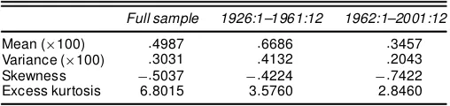
5.1.1 Data. We examine the monthly excess returns on the most comprehensive CRSP value-weighted index (includ-ing dividends)—the monthly continuously compounded return on the index minus the monthly return on the 30-day Treasury Bills—over the period January 1926–December 2001. The data were obtained from the CRSP, which includes the New York Stock Exchange (NYSE), American Stock Exchange (AMEX), and NASDAQ and is perhaps the best readily available proxy for “the market.” We also conducted an analysis on the Stan-dard & Poor (S&P) 500 series and obtained similar results. The data are plotted in the top panel of Figure 1. Table 1 reports sample moments for the data over the whole sample and two subsamples, each containing approximately half of the data: I (1926–1961) and II (1962–2000).
There is strong evidence of leptokurtosis and negative skew-ness in the full sample and in both subsamples. The table re-veals some differences in moments across subsamples. In par-ticular, the rst subperiod has much higher mean and variance, more pronounced negative skewness, and fatter tails than the rest of the sample. The standard deviation is approximately 10 times the size of the mean, which appears to support the widely held view that it is fundamentally difcult to estimate any mean effect in the presence of such large volatility. How-ever, from a nonparametric standpoint, this evidence is not by itself convincing, because the global moments are one end of the smoothing spectrum where bandwidth is innite, and the other end of the smoothing spectrum is where bandwidth is 0 and corresponds to the point mean being equal to the observa-tion itself and the point standard deviaobserva-tion being the same quan-tity. To illustrate this point, we computed a running mean and running standard deviation with seven observations and equal weighting. The results, shown in the bottom two panels of Fig-ure 1, reveal the time-varying natFig-ure of the mean and volatil-ity. At this frequency, the mean and standard deviation are
much closer in magnitude. Note also that this approach to es-timating volatility provides estimates similar to those obtained from the dynamic models that we propose. In both cases, es-timated volatility is high around well-known events, including the depression years, World War II, the oil shock, and the 1987 crash.
5.1.2 Estimation. We rst discuss some model selection choices that had to be made. For the series estimator, values of the tuning parameters of up to 3 were considered with the models selected by the Akaike information criterion (AIC), which maximizes 2 lnL.!/¡2k, wherekis the number of pa-rameters in the model, and the Bayesian information criterion (BIC), which maximizes 2 lnL.!/¡klnT. These two crite-ria gave somewhat conicting results, but both like the model with pD2, qD1, and MD1. For the EGARCH-M model, AIC choosespD1 andqD3, whereas BIC choosespD1 and
qD1. The selected model is the second choice for both criteria. For the model with Fourier terms, AIC choosespD2,qD1, andMD2, whereas BIC choosespD1,qD1, andMD0. The selected model is only marginally worse than these preferred ones. The valuespD2 andqD1 were also chosen by Nelson (1991).
We chose the same values of pandq when estimating the model using the kernel approach. (Results for other choices of
p and q are available from the authors on request.) It is dif-cult to compare the t of the model estimated with the ker-nel for various values ofpandq, because the models are then nonnested. As explained earlier, the bandwidth was selected by cross-validation over a grid of potential bandwidths. The band-width has the form
±Dk¾ .ht/T¡
1
5; (17)
where¾ .ht/is the standard deviation ofht, updated at each
iter-ation to reect the new estimates ofht. The bandwidth constant
kis allowed to vary between .5 and 2.5 in increments of .1, and the estimated value ofk is the one that produces the highest value of the cross-validated likelihood. We set the values ofh
andhNat¡10 and¡2, based on the results from kernel estima-tion, which does not impose such restrictions. We also check to ensure that no value ofht lies outside of these values in the
course of optimization.
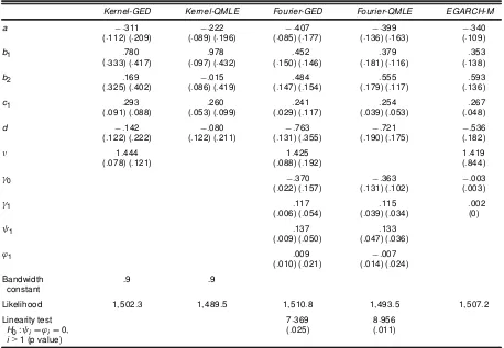
We now turn to the estimation results. The results from the estimation using the two methods considered here and their associated standard errors .seÁ.Á// are presented in Table 2.
Our parameter estimates appear quite robust to the estimation method chosen. They are also consistent with many other stud-ies in the area (e.g., Nelson 1991; Glosten, Jagannathan, and Runkle 1993; Bollerslev et al. 1994). In particular, volatility persistence is quite high (the sum of the estimates ofb1 and b2is well over .9), and the estimate of the leverage effectdis
negative. But this parameter is not precisely estimated with the kernel procedure and is not signicantly different from 0. Fi-nally, the estimated value ofºis around 1.4, which is again con-sistent with previous ndings. The innovation density we nd has fatter tails than a normal sinceº <2. Note that the boot-strap standard errors tend to be larger than the analytic standard errors, sometimes dramatically so. The QMLE standard errors are not appreciably different from those obtained from GED es-timation.
Figure 1. Data. (a) A time plot of the continuously compounded returns on the CRSP value-weighted index, 1926–2001. (b) A rolling mean estimate of the risk premium obtained as a moving average using a window width of seven and equal weighting. (c) A rolling estimate of the standard deviation of the excess returns also using a window width of seven observations and equal weighting.
The last row of Table 2 lists results of a likelihood ratio test for the signicance of the coefcients on the nonlinear terms in the Fourier series. The results clearly show that linearity is strongly rejected at usual signicance levels.
Table 1. Raw Data by Subperiod
Full sample 1926:1–1961:12 1962:1–2001:12
Mean (£100) :4987 :6686 :3457 Variance (£100) :3031 :4132 :2043 Skewness ¡:5037 ¡:4224 ¡:7422 Excess kurtosis 6:8015 3:5760 2:8460
NOTE: Descriptive statistics for monthly excess returns on the CRSP value-weighted index for the entire sample (1926:1–2001:12) and two subsamples (1925:1–1961:12) and (1962:1– 2001:12). The skewness and excess kurtosis are obtained after standardizing excess returns
as(rt¡r ft)¡¹
¾ , where¹and¾are the mean and standard deviation of excess returns over the
relevant sample. Skewness is computed as the sample third moment of the standardized ex-cess returns; exex-cess kurtosis, as the sample fourth moment of the standardized exex-cess returns minus 3. Excess kurtosis would be 0 for a normal distribution.
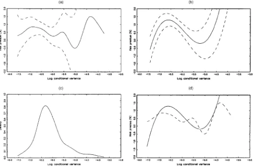
The risk premium estimated using the kernel method is graphed in Figure 2(a) as a function ofht. Condence
inter-vals at the 95% level constructed using the pointwise kernel condence intervals are also provided. The gure clearly re-veals a nonmonotonicrelation betweenhtandE[ytjFt¡1]. This
is consistent with the ndings of Backus and Gregory (1993), Whitelaw (2000), and Veronesi (2001) that in general equilib-rium the risk premium may have virtually any shape. Although the estimated risk premium is not signicantly different from a constant at this level for some part of its range, the evidence is stronger in the middle rangeht2[¡7:5;¡5:5], which is where
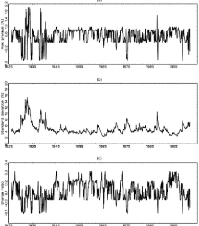
most of the data lie (Figure 2(c) plots the marginal density). The negative values of the risk premium for some values of the state are not statistically signicant. The evolution of the estimated risk premium, conditional standard deviation, and Sharpe ra-tio (in monthly terms) are illustrated in Figure 3. The episodes of high volatility revealed by this gure coincide closely with those obtained by a simple running average, as is done in
Table 2. Full Sample Estimates
rt¡rtfD¹tC¾t"t
htDln (¾t2)DaCb1ht¡1Cb2ht¡2Cc1(|"t¡1|¡E|"t¡1|¡d"t¡1) Fourier:¹tD°0C°1h¤tCÃ1sin (h¤
t)C’1cos (h¤t) "tsGED(º) or N(0;1)
Kernel-GED Kernel-QMLE Fourier-GED Fourier-QMLE EGARCH-M
a ¡:311 ¡:222 ¡:407 ¡:399 ¡:340
(:112) (:209) (:089) (:196) (:085) (:177) (:136) (:163) (:109)
b1 :780 :978 :452 :379 :353
(:333) (:417) (:097) (:432) (:150) (:146) (:181) (:116) (:138)
b2 :169 ¡:015 :484 :555 :593
(:325) (:402) (:086) (:419) (:147) (:154) (:179) (:117) (:136)
c1 :293 :260 :241 :254 :267
(:091) (:088) (:053) (:099) (:029) (:117) (:039) (:053) (:048)
d ¡:142 ¡:080 ¡:763 ¡:721 ¡:536
(:122) (:222) (:122) (:211) (:131) (:355) (:190) (:175) (:182)
º 1:444 1:425 1:419
(:078) (:121) (:088) (:192) (:844)
°0 ¡:370 ¡:363 ¡:003
(:022) (:157) (:131) (:102) (:003)
°1 :117 :115 :002
(:006) (:054) (:039) (:034) (0)
Ã1 :137 :133
(:009) (:050) (:047) (:036)
’1 :009 ¡:007
(:010) (:021) (:014) (:024)
Bandwidth .9 .9
constant
Likelihood 1;502:3 1;489:5 1;510:8 1;493:5 1;507:2
Linearity test 7:369 8:956
H0:ÃiD’iD0; (:025) (:011)
i>1 (p value)
NOTE: Empirical estimates of the semiparametric EGARCH model for monthly excess returns on the CRSP value-weighted index for the entire sample (1926–2001). The numbers in parentheses are analytical and wild bootstrap standard errors. For the GED, the analytical standard errors are from the outer product of gradient (OPG); for the QMLE, the analytical standard errors are those of Bollerslev and Wooldridge (1992).
ure 1. Note that stocks were a great deal in the 1990s according to the Sharpe ratio, but that they have become much less so in recent years.
Figure 2(b) provides the shape of the risk premium estimated using the Fourier series. The graph also includes the analyti-cal 95% condence intervals conditional onht. Again, the
esti-mated shape is nonlinear.
The two smoothing methods have advantages and disadvan-tages. The kernel estimate appears quite imprecise in the end-points where there is not much data, as evidenced by the large standard errors and the volatile point estimates. The Fourier series method, on the other hand, is very smooth and gives the appearance of being precisely estimated. However, there is a pronounced upward slope at the high end, which seems at odds with the kernel method nding. This end trend is quite symptomatic of these polynomial-based methods, and we view it with some skepticism. Note also the difference in the stan-dard errors for the two methods. The condence band for the Fourier series method is almost the same width throughout the shown range, whereas the condence band for the kernel is very wide at the end points, reecting the relative paucity of the data in this region. Thus the Fourier series condence
band gives the appearance of being very precisely estimated in a region where we have little data. This is because it is a global tting method that draws its estimates from all of the data. We thus redraw the two estimates on the same plot in the bottom right corner of Figure 2(d). The methods agree quite closely; there is a hump shape that is rst concave and then convex.
Finally, we provide some diagnostics on the standardized residuals"OtD.yt¡ O¹t/=¾Ot. We report the results for just the
ker-nel; similar results have been obtained for the series approach. The plots of the autocorrelogram of both the residuals and their squares indicate that they are close to white noise; there are 4 signicant autocorrelation coefcients at the 5% level among the rst 100 lags in the levels and 5 signicant autocorrelations in the squares.
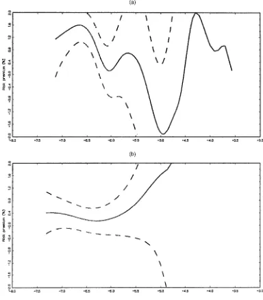
5.1.3 Subsample Estimation. To see how robust our es-timates are, we reestimated the model over two subsamples (1926–1961 and 1962–2001) using the kernel method. The re-sults are presented in Table 3 (with analytical standard errors in parentheses).
The results show quite a bit of instability in the point esti-mates. Figure 5 illustrates the estimated risk premium using the
Figure 2. Empirical Results for the Full Sample. (a) The kernel estimate of the risk premium as a function of the log-conditional variance. The solid line represents the point estimate, and the dashed lines are the limits of a 95% condence interval computed using (14). (b) Similar to (a) but using the Fourier series estimator. (c) The marginal density of the log conditional variance. (d) The point estimates from the kernel and Fourier series. Note that the horizontal scale is the same for all panels and that the vertical scale is the same for all panels except the (c).
same scale as in the other gures. Because the second subsam-ple is characterized by lower volatility than the rst one, the estimated log-volatility is concentrated toward the left of the graph for that period. The estimated risk premium of the sec-ond period is much atter than that of the rst period because of the much larger bandwidth constant chosen, although the point estimate suggests a similar nonmonotonic shape as for the full sample and the rst subsample.
5.2 Monte Carlo
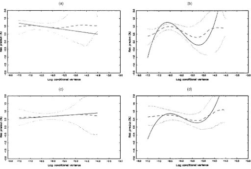
To appreciate the performance of our kernel procedure in es-timating the risk premium in nancial data, we carried out four simulation experiments. We repeated each experiment 5,000 times on samples of size 500. To make the experiments as realistic as possible. We set the parameters of each experi-ment to values estimated from our dataset. The data-generating processes used for the experiments are presented in Table 4.
Simulation experiment 1 involves generating a risk pre-mium from a linear model. We thus estimated an EGARCH-M model with GED errors from the data (results presented in the last column of Table 2) and used it to generate 5,000 sam-ples. We then applied our nonparametric procedure to these simulated samples. The results are presented in Figure 6(a). The solid line represents the true risk premium, which is lin-ear. The long-dashed line is the median estimated function
at each point on our equispaced grid. The short-dashed lines represent the 25th and 75th percentiles. The method appears to do quite well; the median estimate deviates from the true function marginally for all values of the log-conditional vari-ance. The interquartile range of the estimates is relatively narrow in the middle of the distribution, but increases dra-matically for large or small volatility because there is less data.
Experiment 2 uses the model estimated by the Fourier se-ries and GED errors presented in the previous section to gen-erate the data. The results for this experiment are shown in Figure 6(b). The kernel procedure unveils the nonlinear mean function well except for small log-conditionalvariance.
Experiment 3 is a GARCH-M model with normal errors and linear mean. This experiment is designed to check the robust-ness of our results to misspecication in the conditional vari-ance process and the innovationdensity (the parametric compo-nents of our model). The results are shown in Figure 6(c). The kernel procedure discovers the linear mean very well; however, the condence bands are very wide, reecting the additional uncertainty caused by misspecication.
Finally, experiment 4 consists of a GARCH model with nor-mal errors and mean function estimated with Fourier series. Once again, the mean function is well estimated where most data lies, but the uncertainty is once again large due to misspec-ication.
Figure 3. Time Plots of Kernel-Estimated Risk Premium (a), Standard Deviation, (b) and Sharpe Ratio (c). The results are in monthly terms and have not been annualized.
Table 5 presents the median and interquartile ranges for the estimated parameters over the 5,000 replications. Some of these parameters are difcult to interpret, because the es-timated model is misspecied in experiments 3 and 4. For experiments 1 and 2, in which the model is correctly speci-ed, the procedure estimates most parameters well. It has a tendency to underestimate c1, the effect of past innovation
on the log-conditional variance. Also, it does not distinguish well between the effect of ht¡1 and ht¡2 individually in
ex-periment 2, although the overall persistence is well estimated. For the two misspecied models in which data are generated from a GARCH(1,1) model, the parameter values appear rea-sonable, suggesting a single lag of ht¡1 and no leverage
ef-fect. Moreover, the normality of the innovations is well discov-ered.
Overall, these results suggest that our kernel procedure per-forms well in uncoveringpossible nonlinearities in the data, and yet if the model were truly linear, the procedure would not mis-lead us. It is thus a useful tool for examining the shape of the risk premium.
6. CONCLUSIONS
We have found a highly nonlinear relationship between the rst two moments of index returns as suggested by Backus and Gregory (1993) and Gennotte and Marsh (1993). In particu-lar, the risk premium appears to be nonmonotonic and indeed hump-shaped. This result appears to be quite robust to the es-timation method and the tuning parameters selected. However, the estimated risk premiums are subject to quite a bit of vari-ability and are not uniformly signicantly different from 0 at
Figure 4. Autocorrelation of Standardized Residuals and Their Squares. (a) The autocorrelation function of the standardized residuals obtained from the kernel estimator for the rst 100 lags along with the asymptotic 95% condence bands under independence. (b) The same information for the squared standardized residuals.
Table 3. Subperiod Estimates
1926–1961 1962–2001
a ¡:135 ¡:754
(:088) (:216) (:473) (:718)
b1 1:137 :469
(:468) (:465) (:334) (:488)
b2 ¡:159 :411
(:460) (:454) (:333) (:467)
c1 :223 :341
(:118) (:116) (:137) (:108)
d ¡:098 ¡:244
(:165) (:779) (:229) (:476)
º 1:444 1:487
(:125) (:177) (:107) (:194) Bandwidth constant .7 2.5
Likelihood 680.7 829.9
NOTE: See Table 2 note.
the 95% level. This and some instability over time must temper our interpretations to some degree.
ACKNOWLEDGMENTS
We thank Adrian Pagan; participants at the 1999 EC^2 con-ference in Madrid and at seminars at Montréal, Queen’s Uni-versity, and University of California, Santa Barbara; an asso-ciate editor, and two anonymous referees for comments and discussion. Perron acknowledges nancial assistance from the Fonds pour la Formation des chercheurs et l’aide à la recherche (FCAR) and the Mathematics of Information Technology and Complex Systems (MITACS) network. Linton thanks the ESRC and STICERD for nancial support.
[Received September 2000. Revised December 2002.]
Figure 5. Subsample Results. The gure provides kernel estimates of the risk premium for the two subsamples along with the 95% condence bands. The scales are identical to those in Figure 2. (a) Results for the rst subsample, 1926:1–1961:12. (b) The same information for the second subsample, 1962:1–2001:12.
Table 4. Results From Simulation Experiments Data-Generating Processes
Experiment 1: Linear mean, EGARCH conditional variance, and GED errors
¹tD ¡:003¡:002ht
htD ¡:340C:353ht¡1C:593ht¡2C:267(|"t¡1|¡E|"t¡1|¡:536"t¡1)
"tsGED(1:419)
Experiment 2: Fourier mean, EGARCH conditional variance, and GED errors
¹tD ¡:370C:117h¤
t C:137 sin (h¤t)¡:009 cos(h¤t)
htD ¡:407C:452ht¡1C:484ht¡2C:241(|"t¡1|¡E|"t¡1|¡:763"t¡1)
"tsGED(1:425)
Experiment 3: Linear mean, GARCH conditional variance, and normal errors
¹tD:013C:001ht
¾t2D7:402£10¡5C:867¾t2
¡1C:109ut2¡1 "tsN(0;1)
Experiment 4: Fourier mean, GARCH conditional variance, and normal errors
¹tD ¡:229C:073h¤
t C:082 sin (h¤t)¡:006 cos(h¤t) ¾t2D7:163£10¡5C:867¾2
t¡1C:117ut2¡1
"tsN(0;1)
Figure 6. Monte Carlo Results. This gure reports the results on the estimated risk premium from the four simulation experiments: (a) linear mean, EGARCH, and GED errors; (b) Fourier mean, EGARCH, and GED errors; (c) linear mean, GARCH, and normal errors; and (d) Fourier mean, GARCH, and normal errors. In each panel, the solid line is the true relationship, the long-dashed line is the median among the 5,000 replications and the short-dashed lines are the 25th and 75th percentiles. The scales are the same as those in Figures 2 and 5.
Table 5. Results from Simulation Experiments: Median Estimated Parameters
Experiment 1 Experiment 2 Experiment 3 Experiment 4
a ¡:340 ¡:382 ¡:273 ¡:181 (¡:489;¡:267) (¡:598;¡:242) (¡:417; ¡:146) (¡:326; ¡:086)
b1 :375 :715 :890 :978
(:352; :766) (:415; 1:155) (:423;1:351) (:596; 1:391)
b2 :545 :190 :045 ¡:027 (:148; :593) (¡:219; :494) (¡:402; :498) (¡:429; :348)
c1 :216 :136 :199 :196
(:129; :267) (:081; :199) (:122; :267) (:120; :237)
d ¡:536 ¡:838 ¡:029 ¡:010 (¡:823;¡:444) (¡1:335;¡:531) (¡:211; :123) (¡:160; :137)
º 1:419 1:411 1:969 1:981
(1:346;1:460) (1:325;1:506) (1:813; 2:136) (1:833; 2:143)
NOTE: Entries are the median of the estimated parameters over the 5,000 replications. The entries in parentheses are the 25th and 75th percentiles over the 5,000 replications.
REFERENCES
Abel, A. B. (1987), “Stock Prices Under Time-Varying Dividend Risk: An Ex-act Solution in an Innite-Horizon General Equilibrium Model,”Journal of Monetary Economics, 22, 375–393.
(1999), “Risk Premia and Term Premia in General Equilibrium,” Jour-nal of Monetary Economics, 43, 3–33.
Audrino, F., and Bühlmann, P. (2001), “Tree-Structured GARCH Models,”
Journal of The Royal Statistical Society, 63, 727–744.
Backus, D. K., and Gregory, A. W. (1993), “Theoretical Relations Between Risk Premiums and Conditional Variances,” Journal of Business and Eco-nomic Statistics, 11, 177–185.
Backus, D. K., Gregory, A. W., and Zin, S. E. (1989), “Risk Premiums in the Term Structure: Evidence from Articial Economies,”Journal of Monetary Economics, 24, 371–399.
Bollerslev, T., Chou, R. Y., and Kroner, K. F. (1992), “ARCH Modelling in Finance,”Journal of Econometrics, 52, 5–59.
Bollerslev, T., Engle, R. F., and Nelson, D. B. (1994), “ARCH Models,” in
Handbook of Econometrics, Vol. IV, eds. R. F. Engle and D. L. McFadden, Amsterdam: Elsevier Science, pp. 2959–3038.
Bollerslev, T., and Wooldridge, J. M. (1992), “Quasi-Maximum Likelihood Estimation and Inference in Dynamic Models With Time-Varying Covari-ances,”Econometric Reviews, 11, 143–172.
Boudoukh, J., Richardson, M., and Whitelaw, R. F. (1997), “Nonlinearities in the Relation Between the Equity Premium and the Term Structure,” Manage-ment Science, 43, 371–385.
Braun, P. A., Nelson, D. B., and Sunier, A. M. (1995), “Good News, Bad News, Volatility and Betas,”Journal of Finance, 50, 1575–1604.
Breiman, L., and Friedman, J. H. (1985), “Estimating Optimal Transformations for Multiple Regression and Correlation,”Journal of the American Statistical Association, 80, 580–598.
Carrasco, M., and Chen, X. (2002), “Mixing and Moment Properties of Various GARCH and Stochastic Volatility Models,”Econometric Theory, 18, 17–39. Cox, J., Ingersoll, J., and Ross, S. (1985), “An Intertemporal General
Equilib-rium Model of Asset Prices,”Econometrica, 53, 363–384.
Davidson, R., and Flachaire, E. (2001), “The Wild Bootstrap, Tamed at Last,” unpublished manuscript, Queen’s University at Kingston.
Dominitz, J., and Sherman, R. (2001), “Convergence Theory for Stochastic It-erative Procedures With an Application to Semiparametric Estimation,” un-published manuscript, California Institute of Technology.
Engle, R. F., and Gonzalez-Rivera, G. (1991), “Semiparametric ARCH Mod-els,” Journal of Business and Economic Statistics, 9, 345–359.
Engle, R. F., Lilien, D. M., and Robins, R. P. (1987), “Estimating Time Varying Risk Premia in the Term Structure: The ARCH–M Model,”Econometrica, 55, 391–407.
French, K. R., Schwert, G. W., and Stambaugh, R. B. (1987), “Expected Stock Returns and Volatility,”Journal of Financial Economics, 19, 3–29. Gallant, A. R. (1981), “On the Bias in Flexible Functional Forms and an
Essen-tially Unbiased Form: The Fourier Flexible Form,”Journal of Econometrics, 15, 211–245.
Gennotte, G., and Marsh, T. (1993), “Valuations in Economic Uncertainty and Risk Premiums on Capital Assets,”European Economic Review, 37, 1021– 1041.
Glosten, L. R., Jagannathan, R., and Runkle, D. E. (1993), “On the Relation Be-tween the Expected Value and the Volatility of the Nominal Excess Returns on Stocks,”Journal of Finance, 48, 1779–1801.
Gonzalez-Rivera, G., and Drost, F. C. (1999), “Efciency Comparisons of Maximum-Likelihood Based Estimators in GARCH Models,”Journal of Econometrics,93, 93–111.
Hamilton, J. D. (1994),Time Series Analysis, Princeton, NJ: Princeton Univer-sity Press.
Härdle, W. (1990),Applied Nonparametric Regression, Cambridge, U.K.: Cam-bridge University Press.
Härdle, W., and Linton, O. (1994), “Applied Nonparametric Methods,” in
Handbook of Econometrics, Vol. IV, eds. R. F. Engle and D. L. McFadden, Amsterdam: Elsevier, pp. 2295–2339.
Harvey, C. (2001), “The Specication of Conditional Expectations,”Journal of Empirical Finance, 8, 573–638.
Hastie, T., and Tibshirani, R. (1990),Generalized Additive Models, New York: Chapman and Hall.
Lee, S., and Hansen, B. (1994), “Asymptotic Theory for the GARCH(1,1) Quasi-Maximum Likelihood Estimator,”Econometric Theory, 10, 29–52. Lintner, J. (1965), “The Valuation of Risky Assets and the Selection of Risky
Investment in Stock Portfolios and Capital Budgets,”Review of Economics and Statistics, 47, 13–37.
Lumsdaine, R. L. (1996), “Consistency and Asymptotic Normality of the Quasi-Maximum Likelihood Estimator in IGARCH(1,1) and Covariance Stationary GARCH(1,1) Models,”Econometrica, 64, 575–596.
Mammen, E., Linton, O., and Nielsen, J. P. (1999), “The Existence and As-ymptotic Properties of a Backtting Projection Algorithm Under Weak Con-ditions,”The Annals of Statistics, 27, 1443–1490.
Merton, R. C. (1973), “An Intertemporal Capital Asset Pricing Model,” Econo-metrica, 41, 867–887.
Nelson, D. B. (1990), “Stationarity and Persistence in the GARCH(1,1) Model,”
Econometric Theory, 6, 318–334.
(1991), “Conditional Heteroscedasticity in Asset Returns: A New Ap-proach,”Econometrica, 59, 347–370.
Newey, W. K., and Steigerwald, D. G. (1997), “Asymptotic Bias for Quasi-Maximum Likelihood Estimators in Conditional Heteroskedasticity Mod-els,”Econometrica, 65, 587–599.
Opsomer, J. D., and Ruppert, D. (1997), “Fitting a Bivariate Additive Model by Local Polynomial Regression,” The Annals of Statistics, 25, 186–211.
Pagan, A. R., and Hong, Y. S. (1990), “Non-Parametric Estimation and the Risk Premium,” inNonparametric and Semiparametric Methods in Econo-metrics and Statistics: Proceedings of the Fifth International Symposium in Economic Theory and Econometrics, eds. W. A. Barnett, J. Powell, and G. Tauchen, Cambridge, U.K.: Cambridge University Press, pp. 51–75. Pagan, A. R., and Ullah, A. (1999),Nonparametric Econometrics, Cambridge,
U.K.: Cambridge University Press.
(1998), “A Monte Carlo Comparison of Non-Parametric Estimators of the Conditional Variance,” unpublished manuscript, University of Montréal. Perron, B. (in press), “Semi-Parametric Weak Instrument Regressions With an Application to the Risk-Return Trade-Off,”Review of Economics Statistic, 85, 424–443.
Powell, J. (1994), “Estimation of Semiparametric Models,” inHandbook of Econometrics, Vol. IV, eds. R. F. Engle and D. L. McFadden, Amsterdam: Elsevier, pp. 2443–2521.
Robinson, P. M. (1983), “Nonparametric Estimators for Time Series.”Journal of Time Series Analysis,4, 185–207.
(1988), “Root-N–Consistent Semiparametric Regression.” Economet-rica, 56, 931–954.
Sharpe, W. (1964), “Capital Asset Prices: A Theory of Market Equilibrium Un-der Conditions of Risk,”Journal of Finance, 19, 567–575.
Silverman, B. W. (1986),Density Estimation for Statistics and Data Analysis, New York: Chapman and Hall.
Tadikamalla, P. R. (1980), “Random Sampling From the Exponential Power Distribution,”Journal of the American Statistical Association, 75, 683–686. Veronesi, P. (2001), “How Does Information Quality Affect Stock Returns?”
Journal of Finance, 55, 807–837.
Weiss, A. (1986), “Asymptotic Theory for ARCH Models: Estimation and Test-ing,”Econometric Theory,2, 107–131.
Whitelaw, R. F. (2000), “Stock Market Risk and Return: An Equilibrium Ap-proach,”Review of Financial Studies, 13, 521–547.
Wooldridge, J. M. (1994): “Estimation and Inference for Dependent Processes,” inHandbook of Econometrics, Vol. IV, eds. R. F. Engle and D. L. McFadden, Amsterdam: Elsevier, pp. 2659–2738.