A Game-Theoretic Explanation of the
√
dt
Effect
Vladimir Vovk and Glenn Shafer
$25
$0
$50
$0
$100
The Game-Theoretic Probability and Finance Project
Working Paper #5 (preliminary version)
January 27, 2003
Project web site:
Abstract
The returns from a traded security typically have the order of magnitude√dt. This can be explained by the absence of riskless opportunities for making money: any different order of magnitude would permit such opportunities. The expla-nation has been made rigorous in the standard measure-theoretic framework for continuous-time probability, but this requires the assumption that the security’s price process follows a particular stochastic process (usually fractional Brown-ian motion). This note makes the explanation rigorous without any stochastic assumption, using our purely game-theoretic framework for finance [7]. This is a preliminary draft.
Contents
1 Introduction 1
2 Nonstandard results 2
3 Absolute finitary result 4
4 Relative finitary result 5
5 Empirical studies 6
6 Axiom of continuity for upper probability? 9
1
Introduction
The returns from a traded security typically have the order of magnitude√dt. This can be explained by the absence of riskless opportunities for making money: any different order of magnitude would permit such opportunities. It is easy to elaborate this explanation at an intuitive level, where one speaks freely about infinitesmals, because very simple strategies are sufficient to take advantage of returns with an order of magnitude different from √dt. In this note, we show how to translate the intuitive explanation into the purely game-theoretic framework for probability and finance developed in our book, Probability and Finance: It’s Only a Game! [7].
Our game-theoretic result should be compared with analogous measure-theoretic results obtained by Rogers [6], Delbaen and Schachermayer [4], and Cheridito [1, 2]. We rely on the same intuition as these authors,1but our result,
in contrast to their results, does not rely on stochastic assumptions. In order to use the measure-theoretic framework, one must assume that the price of the security follows some stochastic process, and for technical reasons one usually considers some very narrow class of processes, such as fractional or exponential fractional Brownian motion.
As we explain in Appendix 11.5 of our book, our continuous-time framework is an infinitary game. Intuitively, it is a game with an infinite number of rounds
N, each taking an infinitesmal period of time dt, during which the price S
of the security changes by dS. Mathematically, it is an ultraproduct of an infinite sequence of finitary games, which divide a finite time period [0, T] into shorter and shorter trading periods. (The same notion of ultraproduct is used in nonstandard analysis to construct the hyperreals from countably many copies of the reals.) In this infinitary game, we define thep-variationof a price process
S, for any real numberp >0, as an infinite sum:
varS(p) := N−1
X
i=0
|dSn|p.
(We use the notation of [7]: ∆fn:=fn−fn−1, whiledfn:=fn+1−fn.) There
will be some number, which we designate vexS, such thatvarS(p) is infinite for
p >vexS and infinitesmal for p <vexS. We call vexS thevolatility exponent
forS. The inverse of vexS is theH¨older exponent or theHurst exponent. The statement that the incrementsdShave the order of magnitude√dtbecomes, in this framework, the statement that vex = 2, or that the H¨older/Hurst exponent is 1/2.
We prove our infinitary result in§2, using relatively informal language that can be understood rigorously by those familiar with the idea of an ultraproduct. For those not so familiar with this idea, we provide some additional explanation in an appendix.
1In fact, this note results from Delbaen’s calling our attention to Cheridito’s work in his
In§3 and§4. we give messier forms of our result in a realistic, discrete-time setting. We report the results of (extremely) preliminary empirical studies in
§5. In a final section,§7, we remove the assumption of zero interest rate. This is a preliminary draft. In later drafts, we intend to give more explana-tion of the infinitary game and to further simplify the infinitary picture by using the alternative definition of game-theoretic upper probability zero discussed in Frequently Asked Question #1 at www.probabilityandfinance.com.
2
Nonstandard results
The basic framework is that of Chapter 11: the interval T is split into an infinitely large numberN of subintervals etc.
The Market Protocol
Players: Investor, Market
Protocol: I0:= 1.
Market announcesS0∈R. FORn= 1,2, . . . , N:
Investor announcesMn∈R.
Market announcesSn∈R.
In:=In−1+Mn∆Sn.
Additional Constraint on Market: Market must ensure thatS is
continu-ous.
The definition of zero game-theoretic probability is given on pp. 340–341 of [7]: an eventE has zero game-theoretic probability if for anyK there exists a strategy that, when started with 1, does not risk bankruptcy and finishes with capital at leastK whenEhappens.
We start with a result showing that too low volatility gives opportunities for making money.
Theorem 1 For anyδ >0, the event
vexS <2 & sup
t |
S(t)−S(0)|> δ
has game-theoretic probability zero.
The condition vexS <2 means thatSis less volatile than the Brownian motion and supt|S(t)−S(0)|> δ means thatS should not be almost constant.
Proof This proof is a simple modification of Example 3 in [8], p. 658, and a
Assume, without loss of generality, thatS(0) = 0 (if this is not true, replace
S(t) by S(t)−S(0). Consider the strategyMn := 2CSn, where C is a large
positive constant. With our usual notationdfn:=fn+1−fn, we have
dIn = 2CSndSn=C
¡
d(S2
n)−(dSn)2
¢
and, therefore,
In− I0=CSn2−C
n−1
X
i=0
(dSi)2≈CS2n. (1)
If this strategy starts with 1, the capital at each step n will be nonnegative. Stopping playing at the first step when|Sn|> δ, we make sure thatIN ≥Cδ2,
which can be made arbitrarily large by taking a largeC.
As the proof shows, the condition vexS <2 of the theorem can be replaced by the weakervarS(2) = 0.
Now we complement Theorem 1 with a result dealing with too high volatility.
Theorem 2 For anyD >0, the event
vexS >2 & sup
t |S(t)−S(0)|< D (2) has game-theoretic probability zero.
Proof This proof is a simple modification of a proof in [1, 2]. We again assume
S(0) = 0.
Consider the strategyMn:=−2D−2Sn. Now we have
dIn=−2D−2SndSn=D−2
¡
(dSn)2−d(Sn2)
¢
and, therefore,
In− I0=D−2
n−1
X
i=0
(dSi)2−D−2Sn2 ≥D−
2
n−1
X
i=0
(dSi)2−1
before|Sn| reachesD. If this strategy starts with 1 and stops playing as soon
asSnreachesD, the capital at each stepnwill be nonnegative and, if event (2)
occurs,IN ≥D−2varS(2) will be infinitely large.
As before, the condition vexS >2 can be replaced byvarS(2) =∞.
IfSis a stock price, it cannot become negative, which allows us to strengthen the conclusion of Theorem 2.
Corollary 1 The eventvexS >2has game-theoretic probability zero.
Proof LetK be the constant from the definition of zero game-theoretic
prob-ability (p. 2). The required strategy is the 50/50 mixture of the following 2 strategies: the strategy of Theorem 2 corresponding to D := 2K and the buy-and-hold strategy that recommends buying 1 share ofS at the outset. If supt|S(t)−S(0)| <2K, the first strategy will make Investor rich; otherwise,
3
Absolute finitary result
The protocol for this section is:
The Absolute Market Protocol
Players: Investor, Market
Protocol: I0:= 1.
Market announcesS0∈R. FORn= 1,2, . . . , N:
Investor announcesMn∈R.
Market announcesSn∈R.
In:=In−1+Mn∆Sn.
Now N is a usual positive integer number and there are no a priori con-straints on Market. The following is the “absolute” finitary version of Theo-rem 1.
Theorem 3 Letǫandδbe two positive numbers. If Market is required to satisfy
N
X
i=1
(∆Si)2≤ǫ,
the game-theoretic probability of the event
max
n=1,...,N|Sn−S0| ≥δ (3)
is at mostǫ/δ2.
Proof Assume, without loss of generality, that S0= 0 (replaceSn bySn−S0
if not). Take the same strategyMn := 2CSn, but nowC = 1/ǫ. From (1) we
obtain
In− I0=
1
ǫS 2
n−
1
ǫ
n−1
X
i=0
(dSi)2≥
1
ǫS 2
n−1,
i.e., if the strategy starts with 1,
In ≥
1
ǫS 2
n.
This shows thatIn is never negative; stopping at the stepnwhere|Sn| ≥δ, we
4
Relative finitary result
Now we change our protocol to:
The Relative Market Protocol
Players: Investor, Market
Protocol: I0:= 1.
Market announcesS0>0. FORn= 1,2, . . . , N:
Investor announcesMn∈R.
Market announcesSn>0.
In:=In−1+Mn∆Sn.
As in the previous section,N is a standard positive integer number. Define a nonnegative functionβ by
1
2β(x) =x−ln(1 +x);
so for small|x|,β(x) behaves asx2. The following result is the “relative” finitary
version of Theorem 1; it uses the versions
N−1
Theorem 4 Let ǫ,δ andγ be three positive numbers. If Market is required to
satisfy the game-theoretic probability of the event
max
Proof Assume, without loss of generality, thatS0= 1 (replaceSn bySn/S0 if
not). Since the proof is now slightly more complicated than that in the previous section, we first outline its idea. Roughly speaking, our goal will be to maintain
In close to (lnSn)2 (in the previous sections it was to maintain In close to
We can see that a suitable strategy is
Mn:= 2C
lnSn
Sn
for someC(chosen so that to make sure that the capital process is nonnegative; eventually we will take C = 1/((1 +γ)ǫ)). Expressing 2(lnSn)(dSn)/Sn from
the equality between the extreme terms of the chain (5)–(7), we obtain for the strategyMn:
of bankruptcy), in which case (8)–(9) becomes
In≥
First we consider the absolute setting, although the usual definitions as given in [8] are “relative”. Denote
Rabs
Suppose that we believe, for some reason, that we are going to haveSabs
N ≤σ
andRabs
N ≥δ; therefore,δplays the same role as in Theorem 3 andσplays the
role ofp
ǫ/N. So from Theorem 3 we obtain that we will be able to multiply our capitalδ2/ǫ= (δ/σ)2/N-fold. For another variant of the definitions of
withHconsiderably larger than 1/2. If our guesses δandσare not too far off, we can hope to increase our initial capital by a factor of orderN2H−1
. In the “relative” setup, define
Rrel
If we believe that we are going to haveSrel
N ≤σand R
rel
N ≥δ, we obtain from
Theorem 4 that we will be able to multiply our capital by a factor of
δ2
and our guessesδand σare not too far off, we can again hope to increase our initial capital by a factor of order
N2H−1
. (10)
Some experimental results are given in [8] (§4.4), but we cannot use them directly, since the standard definitions ofR/S analysis are different from ours (the main difference being that the standard definition are centered). Those results, however, suggest that typicallyH>0.5, which was why we concentrated on this case in our discrete-time analysis and empirical studies.
In our experiments we considered, instead ofRabs
N andR
rel
N, |SN −S0|and
|ln(SN/S0)|, respectively, the rationale being that security prices typically
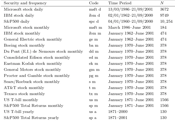
in-crease. This free us from the need to guess the value of δ in advance. Our results are summarized in Tables 1 and 2.
Security and frequency Code Time Period N
Microsoft stock daily msft d 13/03/1986–21/09/2001 3672 IBM stock daily ibm d 02/01/1962–21/09/2000 9749 S&P500 daily spc d 04/01/1960–21/09/2000 10,254 Microsoft stock monthly msft m March 1986–June 2001 184 IBM stock monthly ibm m January 1962–June 2001 474 General Electric stock monthly ge m January 1962–June 2001 474 Boeing stock monthly ba m January 1970–June 2001 378 Du Pont (E.I.) de Nemours stock monthly dd m January 1970–June 2001 378 Consolidated Edison stock monthly ed m January 1970–June 2001 378 Eastman Kodak stock monthly ek m January 1970–June 2001 378 General Motors stock monthly gm m January 1970–June 2001 378 Procter and Gamble stock monthly pg m January 1970–June 2001 378 Sears/Roebuck stock monthly s m January 1970–June 2001 378 AT&T stock monthly t m January 1970–June 2001 378 Texaco stock monthly tx m January 1970–June 2001 378 US T-bill monthly us m January 1871–June 2001 1566 S&P500 Total Returns monthly sp m January 1871–June 2001 1566
US T-bill yearly us a 1871–2000 130
S&P500 Total Returns yearly sp a 1871–2001 130
Table 1: The 19 securities used in our experiments. Dates are given in the format dd/mm/yyyy.
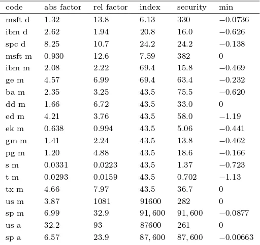
The numbers given in Table 2 are defined as follows:
abs factor := (SN −S0)
2
PN−1
i=0 (dSi)2
and
rel factor :=
³
lnSN
S0
´2
(1−min)³PN−1
i=0 (dlnSi)2 W P N−1
i=0 β
³
dSi
Si
´´,
where
min := min
n ln
Sn
S0.
To judge the magnitude of abs factor and rel factor we also give the factor by which the value of the security increases (the column “security”) and the factor by which the value of an index (S&P500) increases (the column “index”) over the same time period.
code abs factor rel factor index security min msft d 1.32 13.8 6.13 330 −0.0736
ibm d 2.62 1.94 20.8 16.0 −0.626
spc d 8.25 10.7 24.2 24.2 −0.138
msft m 0.930 12.6 7.59 382 0 ibm m 2.08 2.22 69.4 15.8 −0.469
ge m 4.57 6.99 69.4 63.4 −0.232
ba m 2.35 3.25 43.5 75.5 −0.620
dd m 1.66 6.72 43.5 33.0 0 ed m 4.21 3.76 43.5 58.0 −1.19
ek m 0.638 0.994 43.5 5.06 −0.441
gm m 1.41 2.24 43.5 13.8 −0.462
pg m 1.20 4.88 43.5 18.6 −0.166
s m 0.0331 0.0223 43.5 1.37 −0.723
t m 0.0293 0.0159 43.5 0.702 −1.13
tx m 4.66 7.97 43.5 36.7 0 us m 3.87 1081 91600 282 0 sp m 6.99 32.9 91,600 91,600 −0.0877
us a 32.2 93 87600 261 0
sp a 6.57 23.9 87,600 87,600 −0.00663
Table 2: Empirical results related to Theorems 3 and 4.
DJIA cannot be reproduced by a trading strategy) as saying that our initial capital can be increased by a factor of roughly
12,5002×0.59−1
≈5.46
in 12,500 days since 1888.
6
Axiom of continuity for upper probability?
We define upper probabilityP in terms of strategies, and it may not follow from our definitions that it is continuous in the sense
A1⊆A2⊆ · · ·=⇒P
̰ [
i=1 Ai
!
= lim
i→∞P(Ai).
We can, however, “regularize”P replacing it by
P(A) := inf
(
lim
i→∞P(Ai)|A1⊆A2⊆ · · · &A⊆ ∞
[
i=1 Ai
!
.
analogous with Kolmogorov’s axiom of continuity at the time of writing [5]; for further discussion, see www.probabilityandfinance.com. If the game-theoretic axiom of continuity does not lead to counter-intuitive or mathematically awk-ward results, it may be convenient to accept it, but it is too early to make a definitive judgment about its merits yet.
It is clear that the continuity axiom simplifies the above Theorems 1 and 2. We say that an event isfullif its complement has zero regularized game-theoretic probability, and we writeS≈const to mean that supt|S(t)−S(0)|is
infinites-imal.
Theorem 5 The event
vexS= 2or S≈const
is full.
7
Non-zero interest rate
Our protocols implicitly assume that the interest rate is zero. In this section we remove this restriction. Our protocol now involves not only securityS but also another securityB (e.g., a bond). Their prices are assumed nonnegative.
The Market Protocol
Players: Investor, Market
Protocol: I0:= 1.
Market announcesS0>0 andB0>0. FORn= 1,2, . . . , N:
Investor announcesMn∈Rand .
Market announcesSn∈R.
In:= (In−1−MnSn−1)BBn
n−1 +MnSn.
Additional Constraint on Market: Market must ensure that S and B are
continuous.
(Cf. the protocol and its analysis on p. 296 of [7]). Intuitively, at stepnInvestor buys Mn units of S and invests the remaining money in B, which can be a
money market account, a bond, or any other security with nonnegative prices. The protocol of§2 corresponds to a constantBn.
Re-expressing Investor’s capital and the price ofS in thenum´eraire Bn, we
obtain
In† :=In/Bn, Sn† :=Sn/Bn.
It is easy to see that
In† :=I
†
n−1−MnS†n−1+MnSn†,
Theorem 6 The event
vex(S/B) = 2 orS/B≈const
is full.
We have an interesting all-or-nothing phenomenon: either two securities are proportional or their ratio behaves stochastically.
Acknowledgements
The theorems in§2 were inspired by questions raised by Freddy Delbaen in his review of our book in theJournal of the American Statistical Association. Our reply to his review is available at www.probabilityandfinance.com.
Appendix: Details of the proof of Theorem 1
Let us show more formally whyIn is nonnegative and whyIN ≥Cδ2.
According to the first equality in (1), in every finitary structure we have
In−1≥ −C N−1
X
i=0
(dSi)2;
since the value on the right-hand side is infinitesimal (and, therefore, smaller than 1 in absolute value), minnIn is positive.
To see thatIN ≥Cδ2, define in each finitary structure the stopping time
n:= min{i| |Si|> δ}.
Again using the first equality in (1) we obtain that in each finitary structure
IN−1 =In−1 =CSn2−C n−1
X
i=0
(dSi)2> Cδ2−C N−1
X
i=0
(dSi)2;
it remains to remember that the last subtrahend is infinitely small and, there-fore, smaller than 1.
References
[1] Patrick Cheridito. Regularizing fractional Brownian motion with a view towards stock price modelling. PhD thesis, Swiss Federal Institute of Tech-nology, Z¨urich, Switzerland, 2001.
[3] Freddy Delbaen. Review of [7]. Journal of the American Statistical Associ-ation, 97(459), 2002.
[4] Freddy Delbaen and Walter Schachermayer. A general version of the fun-damental theorem of asset pricing. Mathematische Annalen, 300:463–520, 1994.
[5] Andrei N Kolmogorov. Grundbegriffe der Wahrscheinlichkeitsrechnung. Springer, Berlin, 1933. English translation (1950): Foundations of the theory of probability. Chelsea, New York.
[6] L. Chris G. Rogers. Arbitrage with fractional Brownian motion. Mathemat-ical Finance, 7:95–105, 1997.
[7] Glenn Shafer and Vladimir Vovk. Probability and Finance: It’s Only a Game! Wiley, New York, 2001.