www.elsevier.nl / locate / econbase
Why do governments subsidise investment and not
q
employment?
*
Clemens Fuest , Bernd Huber
¨ ¨ ¨
Staatswirtschaftliches Institut, Universitat Munchen, Ludwigstr. 28, VG III, D-80539 Munchen, Germany
Received 1 July 1998; received in revised form 1 May 1999; accepted 1 June 1999
Abstract
The governments of nearly all industrialised countries use subsidies to support the economic development of specific sectors or regions with high rates of unemployment. Conventional economic wisdom would suggest that the most efficient way to support these regions or sectors is to pay employment subsidies. We present evidence showing that capital subsidies are empirically much more important than employment subsidies. We then develop a simple model with unemployment to explain this phenomenon. In our model, unemployment arises due to bargaining between unions and heterogenous firms that differ with respect to their productivity. Union bargaining power raises wage costs and leads to a socially inefficient collapse of low productivity firms and a corresponding job loss. Union–firm bargaining also gives rise to underinvestment. It turns out that an investment subsidy dominates an employment subsidy in terms of welfare if there is bargaining over wages and employment on the firm level. If bargaining is over wages only, results are ambiguous but capital subsidies may still be preferable. 2000 Elsevier Science S.A. All rights reserved.
Keywords: Capital subsidies; Labour subsidies; Unemployment
JEL classification: H20; J51
q
An earlier version of this paper was presented at the Trans-Atlantic Public Economics Seminar (TAPES) on Taxes, Social Insurance, and the Labor Market, May 21–23, Copenhagen.
*Corresponding author. Tel.:149-89-2180-6339; fax:149-89-2180-3128. E-mail address: [email protected] (C. Fuest).
1. Introduction
The governments of nearly all industrialised countries use subsidies to support the economic development of specific sectors or regions with high rates of unemployment. Conventional economic wisdom suggests that the most efficient policy would be to reduce the cost of labour, that is to pay employment subsidies. Empirically, however, governments usually rely on investment rather than employment subsidies. In the debate on these subsidy policies, economists have repeatedly argued that the concentration of public support on investment schemes is inefficient. One example is the case of Eastern Germany, where, in spite of very high rates of unemployment, subsidy programmes almost exclusively support investment. Sinn and Sinn (1993) argue that the public support schemes for Eastern Germany distort the relative price between capital and labour and thus
1
give rise to excessively capital intensive production. They conclude that this policy is suboptimal and that it contributes to the unemployment problem. Begg and Portes (1993) make the same type of argument and conclude that it would be
2
desirable to switch to labour subsidies.
However, while it may well be that investment subsidies are inefficiently high in certain cases, the fact that these subsidies are much more important empirically than employment subsidies seems to be a very general phenomenon. It is therefore unsatisfactory to argue that it simply reflects irrational economic policy decisions. It is the purpose of the present paper to provide an economic explanation for the dominance of investment relative to employment subsidies. We analyse the issue of investment versus employment subsidies in a simple model where unemploy-ment arises due to bargaining between unions and heterogenous firms, which differ with respect to their productivity. Union bargaining power raises wage costs and leads to a socially inefficient liquidation of firms with low productivity and a corresponding loss of jobs. As in Grout (1984), however, union–firm bargaining also leads to underinvestment. In this framework, it turns out that investment subsidies dominate employment subsidies in terms of welfare. The reason is that investment subsidies are a more efficient instrument to alleviate the underinvest-ment problem and to raise the number of operating firms. This result is derived in a model where unions and firms bargain over both wages and employment, i.e., a variant of the efficient bargaining model. We also study the case of a right-to-manage model, where bargaining is over wages only while firms set employment. In this context, it is in general ambiguous whether employment or investment subsidies are to be preferred. We provide a simple example where the dominance of investment subsidies also holds in this framework.
We proceed as follows. Section 2 provides empirical evidence on the role of
1
See also Sinn (1995).
2
employment and investment subsidies in industrialised countries. In Section 3, possible explanations for the dominance of investment incentives are discussed. In Section 4, we develop the model sketched above. In Section 5, we compare the effects of investment and employment subsidies. Section 6 contains the discussion of the right-to-manage model. Finally, conclusions are given in Section 7.
2. Investment and employment subsidies: empirical evidence
In this section, we present some empirical evidence about the role of investment and employment subsidies in industrialised countries. Somewhat surprisingly, there are few empirical studies trying to assess quantitatively the relative importance of these two types of subsidies. In the following, we discuss the results of two studies. Firstly, on the basis of data collected by the OECD (1996), we consider the structure of aggregate general public support to industry in the OECD countries. Secondly, we briefly consider the case of East Germany, based on data
¨
provided by the Sachverstandigenrat / German Council of Economic Advisers
3
(1995 / 96). In both cases, regional or sectoral subsidies are analysed. Subsidisa-tion of employment and investment is measured relative to the general tax and social security system in the various countries under consideration. Our approach thus identifies how policies for specific sectors or regions are designed.
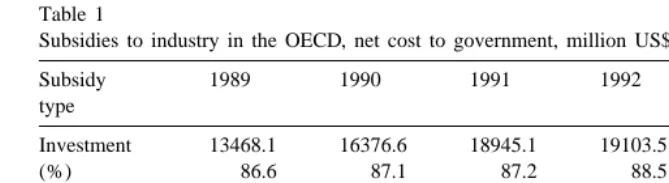
The most comprehensive international study of public support policies is provided by the OECD (1996). This study covers 1552 public support pro-grammes, all aiming at the manufacturing sector, in 24 OECD member countries, the Slovak republic and at the EU level. The study classifies the subsidy programmes, among other things, according to ‘policy objectives pursued’ and ‘economic activities supported’. In this classification, 40% of all subsidies can be assigned to the groups of employment or investment-promoting policies. The remaining 60% mainly comprise research and development and export promotion subsidies, which cannot unambiguously be considered as supporting specifically either employment or investment. The absolute and relative shares of investment and employment subsidies of the remaining 40% of overall subsidies are reported in Table 1.
It turns out that, between 1989 and 1993, around 87% of these subsidies were directed towards the support of investment, whereas only about 13% were devoted to supporting employment. In absolute terms, expenditure on investment-promot-ing measures in the OECD was thus roughly six times as high as expenditure on
3
Table 1
a
Subsidies to industry in the OECD, net cost to government, million US$
Subsidy 1989 1990 1991 1992 1993
type
Investment 13468.1 16376.6 18945.1 19103.5 17754.7
(%) 86.6 87.1 87.2 88.5 88.9
Employment 2084.1 2422 2783.4 2482.3 2208.4
(%) 13.4 12.9 12.8 11.5 11.1
Total 15552.2 18798.6 21728.5 21585.8 19963.1
(%) 100 100 100 100 100
a
Source: OECD (1996); own calculations.
4
programmes promoting employment. Even in relation to all subsidies (including the 60% which cannot be classified), programmes promoting investment thus absorbed 36% of overall public support. The authors of the study therefore conclude: ‘‘ . . . this (the large share of investment subsidies, C.F. / B.H.) shows the extent to which manufacturing investment is an engine of economic development and job creation’’ (OECD, 1996, p. 9).
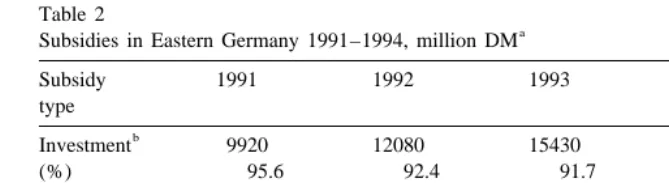
An important case of a specific government subsidy programme, which has received considerable attention among economists, is the transformation of Eastern Germany after reunification. Table 2 gives an overview over the budgetary cost of
5
the most important subsidy programmes for Eastern Germany.
Here, it turns out that over 90% of the expenditure takes the form of investment subsidies, whereas programmes directly promoting employment are almost negli-gible. The figures given above mainly include subsidies for on-the-job training and support for the employment of special groups, such as immigrants of German origin from Eastern Europe. Explicit and general wage subsidy programmes aiming at reducing the cost of labour in Eastern Germany do not exist. Eastern Germany is thus a striking example for the dominance of investment subsidies
6
relative to measures directly promoting employment.
In summary, the empirical evidence given in this paragraph suggests that the preference for investment over employment subsidies is a reasonably general phenomenon. This raises the question of how the dominance of investment
4
The absolute level of subsidies reported in Table 1 seems fairly low. This reflects that the OECD calculates subsidies according to its ‘net cost to government’ (NGC) concept. ‘‘NGC calculates the difference between the cost of funding a programme in any given year and the revenue generated for the public budget by the same programme in any given year’’ (OECD, 1996, p. 12). Of course, such an approach raises various methodological problems that cannot be discussed here.
5
Only the three quantitatively most important measures are covered. For a more detailed account of the investment support policies in Eastern Germany see Sinn (1995).
6
Table 2
a
Subsidies in Eastern Germany 1991–1994, million DM
Subsidy 1991 1992 1993 1994
Source: Sachverstandigenrat / German Council of Economic Advisers (1995 / 96); own calculations.
a
Includes: Investment Allowances according to the Laws on Corporate and Personal Income Taxation, Investment Grants on the basis of the program ‘Common Task: Improvement of Regional Economic Structure’ (Gemeinschaftsaufgabe: Verbesserung der regionalen Wirtschaftsstruktur) and
¨
Special Depreciation Provisions according to the ‘Regional Support Law’ (Fordergebietsgesetz).
c
Includes: Promotion of ‘Starting to Work’, Subsidies for On-the Job Training, Diverse Labour Market Integration Programmes.
subsidies can be explained. Possible answers to this question will be discussed in the following paragraph.
3. The investment subsidy puzzle
The empirical dominance of investment subsidies raises the question of why governments seem to prefer investment to employment subsidies, given that unemployment is almost always a key problem of the supported regions. In fact, in a standard labour market model with rigid wages, it is a straightforward exercise in welfare analysis to show that employment subsidies strictly dominate investment subsidies (Begg and Portes, 1993; Sinn, 1995). The policy implications of this theoretical benchmark case stand in marked contrast to the policy actually pursued by most governments. Before turning to our explanation of this investment subsidy puzzle, we should mention other possible reasons.
One explanation for the higher level of investment subsidies may simply be that employment and investment subsidies have different underlying policy objectives. While employment subsidies clearly have the function to raise employment, investment may be subsidised for reasons not directly related to labor markets. Most importantly, investment subsidies are also an instrument to raise economic growth. The endogenous growth literature has identified various externalities arising from private investment in physical capital. These externalities may justify
7
investment subsidies. Investment grants may also be a result of tax competition,
7
where national governments offer fiscal incentives to attract internationally mobile capital.
A second possible explanation can be found in Torsvik (1993). In the model of his paper, employment subsidies represent a first-best policy. The first-best, however, cannot be implemented because there is a time inconsistency problem. In his model, the government cannot commit to future payments of employment subsidies promised to firms in the present.
Investment subsidies, in contrast, are paid immediately and therefore serve as a substitute for employment subsidies. One might object here that this argument does not explain why the government should not pay out labour subsidies immediately as well, based on future employment as announced by the firms, and raise taxes later if the firm does not fulfil its employment obligations.
Thirdly, one may take a public choice perspective and argue that investment subsidies are a result of rent seeking. For instance, the producers of capital goods, which form a well-defined interest group, may successfully lobby for investment
8
subsidies. Finally, many practitioners argue that, while there may be a theoretical case for wage subsidies, they are much more difficult to administer than investment subsidies.
In what follows, we develop a model which gives a different explanation. In this model, union–firm bargaining distorts both employment and investment decisions and leads to an inefficiently low number of active firms. To correct these distortions, the government may subsidise capital and labour. This model provides a rationale for using investment rather than employment subsidies.
4. A model to explain the investment subsidy puzzle
In this section, we set up a model which will be used to provide an explanation for the investment subsidy puzzle. We proceed as follows. In Section 4.1, the basic structure of the model is presented. In Section 4.2, we discuss the benchmark case of a competitive labour market. In Section 4.3, we derive the equilibrium with union–firm bargaining.
4.1. The basic structure of the model
There are two groups of agents in the economy: entrepreneurs and workers. Each entrepreneur owns a firm which produces a homogeneous numeraire good. The output of firm i is
8
Y(K , L )i i 1zmi (1) where K and L are capital and labour employed by firm i. Y is a strictly concavei i
production function satisfying the standard neoclassical properties. Y(K, L ) is
9
common to all firms whereasmidenotes a firm-specific random output shock; z is a positive parameter. For the economy as a whole, m is assumed to be uniformly distributed with support [0; 1]. For notational convenience, we normalise the number of entrepreneurs and firms to unity.
Each entrepreneur is endowed with K units of capital. This endowment may be0
used either for investment in the firm or for investment in a foreign capital market where it yields the riskless exogenous interest rate r. The entrepreneurs are assumed to be risk-neutral to rule out potential effects of risk-aversion on investment behaviour. In addition, we assume that K is always large enough to0
finance investment in the firm. While this assumption is not critical for our results, it simplifies the analysis by ruling out problems arising from the potential bankruptcy of firms.
Investment, employment and production decisions in this model are not taken simultaneously but in a sequence of three stages. At the first stage, the firms choose the optimal level of investment. At the time of this decision, mi is unknown. Since firms are ex ante identical, all firms choose the same capital stock, which will be denoted by K. At the second stage, the labour market transactions take place. At this time, mi is still unknown. The number of workers (L ) and the wage rate (w) will therefore also be the same for all firms. Note that this particular timing of decisions, where labour market contracts are made after investment decisions have been taken, follows the sequence in the seminal paper of Grout (1984).
At the third stage, mi is finally revealed. Given mi, each firm has to decide whether to take up production or to close down. If the firm produces, the entrepreneur earns Y(L,K )1zm 2i wL. If the firm is closed down, the workers
10
become unemployed and the capital goods are sold. The liquidation of the firm yields (11r )K. We assume r0 .r0. 21, such that, while the liquidation value of the firm is strictly positive, the return from selling the firm’s assets is less than the market rate of interest. A firm i therefore chooses to produce if and only if
Y(K , L )i i 1zm 2i wL$(11r )K .0 i (2)
9
As will become clear in the course of the analysis, this heterogeneity between firms implies that, in the case of a unionised labour market, employment for the economy as a whole is inefficiently low despite efficient bargaining on the firm level.
10
While the entrepreneurs in our economy take investment decisions and manage the firms, there is a second group of agents, the workers. The overall number of workers is N and each worker inelastically supplies one unit of labour such that L denotes the number of workers employed in each firm. Workers have no initial endowment with capital. A worker of a firm which is not liquidated earns the wage rate w, while a worker who finds no job or is employed by a firm which is closed down has an income c, which may also be interpreted as the value of leisure. The workers are assumed to be risk neutral, i.e., they only care about their expected income.
In the following section, we first analyse the benchmark case where no trade union exists, i.e., the case of a competitive labour market. In Section 4.3, we then assume that the workers form trade unions, such that labour contracts are subject to bargaining between unions and firms.
4.2. Equilibrium with competitive labour markets
We determine the competitive equilibrium by solving the model recursively, beginning with the third stage. We first note that, for given values of K, w, and L,
c
(2) determines the critical shock levelm . All firms whose productivity shock turns
c
out to be lower than the critical level m are liquidated because the operating profits (the l.h.s. of (2)) is lower than the liquidation value (the r.h.s. of (2)). As all firms in the economy are assumed to be distributed in the intervalm[ [0; 1], a
c c
corner solution where no firms are liquidated withm 50 may arise. Note thatm is also the ex ante probability that a firm will be closed down at the third stage. Finally, as we have normalised the overall number of firms in the economy to
c
unity,m may also be interpreted as the number of firms which will be liquidated
c
at stage three; hence, the number of producing firms will be 12m.
Consider now the second stage. In a competitive labour market, each firm chooses labour input to maximise net revenue Y1zm 2i wL if production is taken
up. This simply yields the marginal productivity condition YL5w. The equilibrium
wage rate obviously satisfies w$c. The wage rate may exceed c if L5N in the
equilibrium, i.e., no voluntary unemployment exists. For the following analysis, it is useful to concentrate on the case of an interior solution, where the labour market clears with L,N and w5c. The labour market equilibrium can then be described
by
YL5c. (3)
We finally turn to the first stage where the firms choose K. For the analysis of investment behaviour, suppose for the sake of the argument that all firms decide to
c
Y(K , L )i i 1zE(mi)2wL2(11r)Ki
where E(mi)51 / 2 is the expected value ofmi. The first-order condition for K is
YK511r. (4)
c
It remains to be shown thatm 50 holds in equilibrium. To demonstrate this, one can use (3) and (4) to write (2) as
Y(K, L )2Y KK 2Y LL 1(r2r )K0 1zm .i 0
which implies that all firms will take up production. We thus have
c
m 50. (5)
Eqs. (3)–(5) and the condition w5c completely describe the competitive
equilibrium, i.e., the equilibrium values of L, K, w and the liquidation probability
c
m. The competitive equilibrium also represents a first-best outcome in this economy and will serve as a benchmark for the following analysis.
4.3. The equilibrium with union–firm bargaining
We now introduce a trade union which represents the interests of the workers. As the number of firms is normalised to unity, we also consider one representative trade union. In line with the assumption of risk-neutral workers, it is the objective of the union to maximise expected labour income of workers (U ) which is given by
*
U5cN1(12m )(w2c)L (6)
wherem* now denotes the probability that a firm is closed. Of course, the union essentially has the function to raise the wage rate above the competitive wage c. The labour market is now characterised by union–firm bargaining, which takes place at stage two in the sequence of decisions. As in Grout (1984), the union is assumed to know the capital stock (K ). The (representative) union and the (representative) firm bargain over wages (w) and employment per firm (L ). The outcome of this bargaining process specifies a wage–employment contract which
11
determines w and L. We thus assume that there is efficient bargaining on the firm level. An alternative approach would be to assume that bargaining is over wages only, while employment is set unilaterally by firms, as in the right-to-manage model of union–firm bargaining. The question of which is the appropriate bargaining model is an old issue in the theory of unionised labour markets. Both
11
12
approaches can be justified on empirical grounds. While our main results are derived in an efficient bargaining framework, the implications of using the right to manage approach in our model will be discussed in Section 6.
The expected profit (P) of the representative firm in stage 2, where the capital stock is given, can be written as
m
1 *
P5
E
(Y(K, L )1zm 2wL )dm 1E
(11r )K d0 m. (7)m* 0
The first term in (7) captures the profit of a firm which takes up production. This occurs with probability (12m*). The second term is the revenue from a liquidation, which occurs with probability m*.
As in much of the literature on unionised labour markets, we derive the outcome of union–firm bargaining using the Nash-Bargaining solution (Nash, 1950). The Nash maximand is
V 5 blog(U2U )0 1(12b) log(P2P )0 (8)
where (0#b #1) is the relative bargaining power of the trade union. Withb 51, we have the polar case of a monopoly union; b 50 is the opposite case, where the employers hold all bargaining power. U is the union’s outside option, that is the0 13
income level which would be attained if negotiations fail, which is U05cN.
Accordingly, the outside option of the firm (or, more precisely, the entrepreneur) is simply the liquidation value: P05(11r )K.0
As in the preceding section, the equilibrium in this economy is derived recursively. At the third stage (where w, L and K are given), (2) allows to determine the ex ante probability m* that a firm will be closed down. More formally, m* is given by
*
Y(K, L )1zm 2wL$(11r )K0 (9) where (9) holds as a strict equality if m*.0.
Consider now the second stage, where the bargaining between the union and the firm determines w and L (for a given K ). The bargaining parties rationally
12
Empirical evidence in favour of the efficient bargaining model is provided, for instance, by Svejnar (1986). For evidence in favour of the right-to-manage model see Oswald (1993). MaCurdy and Pencavel (1986), who also find evidence in support of the efficient bargaining model, conclude that ‘‘surely, neither of these models is the relevant one in all labor markets at all times.’’ (ibid., p. S34).
13
anticipate that their wage / employment decisions will affect the liquidation probability as in Eq. (9). The bargaining problem is thus to maximise (8) subject to the constraint (9):
*
max L 5 V 1 l(Y(K, L )1zm 2wL2(11r )K )0 (w ;L ;m*;l)
where l is the multiplier for constraint (9) in the Lagrangean L. The first-order conditions can be written as:
(12b)
]]] *
L: b 1(P2P )(12m )(YL2w)L1l(YL2w)L50, (10a)
0
(12b)
]]] *
w: b 2 (12m )(w2c)L2l(w2c)L50, (10b) (P2P )0
(12b)
]]]
* * *
m : b 1(P2P )(12m )(Y(K, L )1zm 2wL2(11r )K )0 0
*
2lz(12m )50. (10c)
We focus on an interior solution form* withm*.0, such that (9) is binding with
l.0 at the optimum. Below, we will derive a sufficient condition form*.0. As a first result, one can see from (10a) and (10b) that
YL5c. (11)
The bargaining solution implies that employment in the producing firms is efficient. Using (10b), (10c) and the (binding) constraint (9), one can now derive
b ]
L(w2c)52(Y(K, L )1z2cL2(11r )K ).0 (12) The term L(w2c) can be interpreted as the rent the union achieves in the
bargaining process. This rent simply turns out to be the fractionb/ 2 of the surplus generated by the most productive firm in the economy (the term on the right-hand side of (12)). A monopoly union (b 51) would capture half of this surplus. If the union has no bargaining power (b 50), its rent is zero.
Consequently, for a given capital stock, and if the union has some bargaining power (b .0), the wage rate under union–firm bargaining will always exceed the wage rate in a competitive labour market. This affects the probability of a firm to be liquidated. To see this, consider the least productive firm in the economy, that is the firm j with m 5j 0. This firm will be closed if
14
The sum of the first three terms is strictly positive. If w5c, firm j will never be
closed, which confirms our result for the competitive labour market, where we
c
have shown that m 50. If w.c, however, the entrepreneur may prefer to close
firm j. Using (12) and making some rearrangements shows that firm j is liquidated if and only if
22b
]]b (Y(K, L )2cL2(11r )K )0 ,z. (13) We assume that (13) is satisfied, which also ensures that we have an interior
15
solution, i.e., thatm*.0 holds in the equilibrium. It is now also straightforward to derive the probability that a firm will take up production (12m*):
22b 22b 1
]] ]] ]
*
12m 5 2 1 2 z(Y(K, L )2cL2(11r )K )0 ,1. (14) Notice that (12m*) is also the number of firms which will take up production in the equilibrium with union–firm bargaining. For a given K, it thus turns out that union–firm bargaining leads to a decline in the number of operating firms relative to the equilibrium with a competitive labour market. This undersupply of firms constitutes the key source of inefficiencies associated with non-competitive labour markets in this model: a firm i will take up production if Y(K, L )1zm 2i wL2
(11r )K0 $0. From a welfare point of view, however, it is desirable to produce as long as Y(K, L )1zm 2i cL2(11r )K0 $0. The undersupply of operating firms also induces an inefficiently low level of employment in the economy because, for a given K, less workers are employed than would be socially optimal. Notice also that the reason for this unemployment is the inefficiently low number of firms; the level of employment within each individual producing firm is efficient since YL5c. These results can be summarised as
Proposition 1. If there is union –firm bargaining, and if the union has some
bargaining power (0,b #1),
1. employment in the operating firms is efficient but
2. the number of operating firms and, hence, employment for the economy as a
whole is inefficiently low.
Proof. See above.
So far, we have discussed stages two and three, where we have derived the
14
This follows from the fact that Y2cL5Y2Y LL .Y K and, as will be shown in the followingK analysis, YK$11r.11r .0
15
equilibrium values of L, w andm* for a given K. For further use, we rewrite these variables as functions of K. Straightforward comparative statics reveal:
Y
≠L KL
]5 2], (15)
≠K YLL
(Y 2(11r )) Y
≠w b K 0 KL (w2c)
]5] ]]]]1] ]], (16)
≠K 2 L YLL L
and
*
≠m 1 22b
]]≠K 5 2] ]]z 2 (YK2(11r )).0 (17) On the basis of the results for stages two and three, we may now discuss investment behaviour at stage one. The firm anticipates the effect of the capital stock on the bargaining outcome, i.e., L, w and m*, and maximizes expected profits (I ) over K:
m* 1
max I5
E
(Y(K; L )1zm 2wL ) dm 1E
(11r )K d0 m 2(11r)K. (18)K
m* 0
We can now immediately state
Proposition 2. If there is union –firm bargaining, and if the union has some
bargaining power (0,b #1) the capital stock is inefficiently low.
16
Proof. The first-order condition of the investor’s problem can be written as
22b ]]
*
(12m ) 2 (YK2(11r ))0 1(11r )0 2(11r)50 (19) which directly implies that we have
2 1
]]] ]]]
YK2(11r )0 5(r2r )0 (22b) (12m*).0 in the equilibrium. Rewriting (19) yields
b ]
S
*D
YK511r1 21m (YK2(11r ))0 (20) which shows that the marginal productivity of capital now exceeds (11r) for
b .0. Relative to the first-best, investment is thus inefficiently low. h
16
Underinvestment occurs because the firms take into account that the benefit of an increase in the capital stock is partly captured by the unions via the bargaining
17
process. This underinvestment problem plays a central role in our analysis and is also the key to understanding why capital subsidies are preferable to labour subsidies in our model. The theoretical finding that unionisation may have a negative impact on investment is also supported by empirical studies for the US (Conolly et al., 1986) and the UK (Denny and Nickell, 1991).
To summarise, the equilibrium which emerges under union–firm bargaining is thus characterised as follows. While employment in the operating firms is efficient, there is underemployment for the economy as a whole because the number of operating firms is inefficiently low. There is also a suboptimal level of investment. The magnitude of these distortions depends on the relative bargaining power of the trade union.
5. Employment versus investment subsidies
The preceding analysis has shown that trade union power gives rise to employment and investment distortions and welfare losses. There is thus a potential role for welfare-enhancing government interventions. Since all agents are risk-neutral, we use aggregate surplus as a welfare criterion.
This surplus (R) can be written as
m
1 *
R5
E
(Y(K; L )1zm 2cL ) dm 1E
(11r )K d0 m 2(11r)K. (21)m* 0
In the present section, we introduce two policy instruments. A capital tax (or, if negative, a subsidy) denoted by t and a payroll tax (or subsidy) which we denote byt. In the Appendix, we integrate these two taxes / subsidies into our model and again derive the equilibrium under union / firm bargaining, as in Section 4.3.
It is straightforward to show that, considered separately, and assuming lump sum financing, the introduction of both subsidy types would raise welfare. This is not particularly surprising. It is the purpose of this paper, however, to compare the efficiency of employment and investment subsidies. In order to make this comparison, we therefore assume that, if an investment subsidy is to be paid, it has to be financed by a tax on labour, and vice versa. The government budget constraint is thus
17
1
E
(tK1twL ) dm 50. (22)m*
Analysing the effect of the two subsidies / taxes on investment, employment, the number of firms and welfare leads to the following results:
Proposition 3. If there is union –firm bargaining, and if the union has some
bargaining power (0,b #1), introducing an investment subsidy financed by a
labour tax
1. raises the capital stock in the operating firms; 2. has an ambiguous effect on overall employment; 3. raises the number of operating firms; and 4. raises welfare.
Proof. See Appendix A.
These results can be explained as follows. Consider first the impact of the capital subsidy, abstracting from the labour tax increase for the moment. The capital subsidy raises investment in the operating firms and improves profitability such that the overall number of firms increases. In addition, the higher capital stock and the higher number of operating firms raise labour demand and employment. Given that both investment and employment are inefficiently low in the initial equilibrium (see Proposition 1), the capital subsidy will therefore raise welfare.
Consider now the impact of the labour tax which is used to finance the capital subsidy. The labour tax c.p. reduces labour demand, investment and employment. This tends to reduce welfare. Our analysis shows, however, that the positive effects of the capital subsidy dominate the negative impact of the labour tax, such
18
that the overall welfare effect is positive. Intuitively, the reason is that the labour tax is partly a tax on the workers’ rents, which are a consequence of union power. Of course, this is a somewhat surprising result and the question arises whether it is robust if some of the underlying assumptions are changed. As mentioned in Section 4.3, one important assumption underlying our analysis is that of efficient
18
bargaining at the firm level. In the next section, we consider the case of the right-to-manage model of wage bargaining.
6. Capital subsidies in the right-to-manage model
In the present section, we consider the welfare effect of capital subsidies in a right-to-manage model. Thus, we now assume that bargaining between unions and firms is over wages only, whereas the level of employment is set unilaterally by firms. To keep the following analysis simple, we normalise the parameter z to zero, which implies that we abstract from firm heterogeneity and the possibility of
19
firm liquidations. The sequence of decisions is now as follows. As in the preceding analysis, the investment decision is taken at stage one and union–firm bargaining takes place at stage two. The crucial new aspect is now, of course, that unions and firms bargain over wages only. At stage three, firms unilaterally set employment.
We determine the equilibrium beginning with stage three. As in the preceding
20
analysis, we first abstract from taxes. At stage three, for a given capital stock, the representative firm maximizes the term
P5Y(L, K )2wL (23)
over L. The firm’s optimal employment decision is
YL5w. (24)
At stage two, firms and unions bargain over wages. The objective function of the representative union is given by
U5wL1(N2L )c (25)
and the union’s reservation utility is cN. The firm’s objective function is given by (23), and its reservation profit is (11r )K. The Nash maximand is thus0
V 5 blog(L(w2c))1(12b) log(Y(L, K )2wL2(11r )K )).0 (26) The wage rate emerging from the bargaining process is derived by maximizing (26) over w. The first-order condition V 5w 0 can be rearranged to yield
21
L
12b L w
]] ]]]]]]]] ]
w2c5
F
b 2G
.0. (27)L
(Y(L, K )2wL2(11r )K )0
19
In the preceding section, the liquidation of low productivity firms was required to have an equilibrium with an inefficiently low level of employment, given the capital stock. Here, the level of employment will be too low even without firm liquidations.
20
Eq. (27) shows that the equilibrium wage rate exceeds the marginal disutility of working (w.c). Eq. (27) also defines the wage rate as a function of the capital
stock, i.e., w5w(K ).
At the first stage, the entrepreneurs choose the level of investment, taking into account that the size of the capital stock will affect the outcome of wage bargaining at stage two. The profit function at stage one is
I5Y(L, K )2w(K )L2(11r)K. (28) Maximizing (28) over K yields
≠w
]
YK5(11r)1≠KL. (29)
Eq. (29) shows that, if an increase in the capital stock raises the wage rate
21
emerging from the bargaining process , entrepreneurs will set K such that the marginal productivity of capital exceeds the ‘social cost’ of capital (11r), which
means that underinvestment occurs. It is now straightforward to determine the welfare effect of introducing a capital subsidy, financed by a labour tax. Overall welfare is
R5Y(L, K )2cL2(11r)K. (30) Let dL and dK denote the change in investment and employment induced by the introduction of a capital subsidy. The change in welfare is then
dR5(YK2(11r)) dK1(YL2c) dL.
Using (24) and (29), this can be written as
≠w
]
dR5≠ L dK1(w2c) dL. (31)
K
Eq. (31) shows that the welfare effect of introducing a capital tax is determined by the resulting (equilibrium) changes of K and L induced by the introduction of the capital subsidy. In a first-best world, a marginal capital subsidy would, of course, not affect welfare. In this model, both investment and employment decisions are distorted such that marginal changes in K and L have a first-order welfare effect. In general, the welfare effect of introducing the capital subsidy (financed by a labour tax) is now ambiguous. In Appendix B, we provide a simple example for a positive welfare effect. If bargaining is over wages only, the case for capital subsidies is thus weaker, but they may still induce a welfare gain.
21
7. Conclusions
It is the purpose of this paper to find an explanation for the empirical observation that governments prefer investment to employment subsidies in policies aiming at the support of regions or sectors with high rates of unemploy-ment. We have compared investment and employment subsidies in a model where union–firm bargaining gives rise to unemployment by reducing the number of active firms in the economy. It turns out that, while no unambiguous conclusions can be drawn for the relative effectiveness of the two subsidies in promoting employment, investment subsidies unambiguously dominate employment subsidies in terms of welfare in our model if the efficient bargaining model applies. In the case of the right-to-manage model, results are ambiguous, but it is possible that capital subsidies are still preferable. It may therefore be misleading to argue that the widespread preference for investment incentives necessarily reflects suboptimal economic policy decisions.
Acknowledgements
The authors would like to thank Ann-Sofie Kolm and John Whalley for very helpful comments and suggestions. Moreover, we are indebted to two anonymous referees and to Søren Bo Nielsen. The paper has also benefitted from discussions with Thorsten Bayindir-Upmann. The usual disclaimer applies.
Appendix A
In this appendix, we derive the equilibrium under union–firm bargaining with the subsidies / taxes t andt. Form*.0, the marginal firm is now characterised by the condition:
*
Y(K; L )1zm 2tK2(11t)wL2(11r )K0 50. (A.1) Expected profits of the representative firm (P) are now
m
1 *
P5
E
(Y(K, L )1zm 2tK2(11t)wL ) dm 1E
(11r )K d0 m. (A.2)m* 0
The objective function of the union does not change. The bargaining solution now yields the following equations:
YL5(11t)c (A.3)
b ]
L(w2c)(11t)5 2(Y(K; L )1z2cL(11t)2(11r01t)K ). (A.4) The investor’s objective function is
m
1 *
I5
E
(Y(K; L )1zm 2tK2(11t)wL ) dm 1E
(11r )K d0 m 2(11r)K.m* 0
(A.5)
The first-order condition of the investor’s problem becomes
≠I (22b)
]≠K5(12m*)]]]2 (YK2(11r01t))111r02(11r)50 (A.6) where we have used
Y
≠L KL
]≠ 5 2].0 (A.7)
K YLL
and
*
≠m 1 22b
]]≠K 5 2] ]]z 2 (YK2(11r01t)),0. (A.8) For later use, we note that the second-order condition requires
2
2 2
Y
≠ I 1 (22b) 2 (22b) KL
]]25] ]]]z 4 (YK2(11r01t)) 1(12m*)]]]2
S
YKK2]]YD
≠K LL
,0 (A.9)
which we assume to hold. The equilibrium is thus characterised by Eqs. (A.1), (A.3), (A.4) and (A.6). We now derive the effect of a simultaneous change in t and
t, departing from an equilibrium with t5t 50. A change in t andt which keeps the budget balanced implies
dt K5 2dtwL. (A.10)
Totally differentiating Eqs. (A.3), (A.4), (A.6), and using the total differential of (A.1) and dt 5 2dt K /wL yields
1 K c
] ] ]
dL5 2Y (YLKdK1L wdt), (A.11)
LL
b 22b c
] ]] ]
b 22
]]2 [dm*(YK2(11r01t))1(12m*)(dt2(YKKdK1YKLdL ))]50. (A.13)
Eqs. (A.11)–(A.13) determine dL, dK and dm* as functions of dt. We thus get
Y
dK 22b KL K c
]5]]
F
(12m*) 1S
1] ] ]D
dt 2 YLL L w
2
1 (22b) c ≠ I
] ]]] ] ]]
1 z 2 (YK2(11r01t))
S
12wD
K 1 /G
2,0 (A.14)≠K
where we assume
YKL K c
] ] ]
11 .0
YLL L w
to hold. For this condition to be satisfied it is sufficient to assume a homogeneous production function with decreasing returns to scale. For the effect on employment per firm, we get
dL 1 dK K c
]dt 5 2]Y
S
YLK]dt 1] ]L wD
(A.15)LL
which is ambiguous but becomes negative if c is small, such that the employment effect of a capital subsidy (dt,0) is positive. Form* (remember that the number of operating firms is (12m*), we have
*
dm 1 (b 22) dK c
]]dt 5] ]]]z 2 ((YK2(11r01t))]dt 2
S
12]wD
K ).0. (A.16) Eqs. (A.14)–(A.16) prove parts 1–3 of Proposition 3. The welfare effect is derived by differentiating Eq. (B.4). It is easy to check that, in the equilibrium, we have≠R ≠R ≠R
]50; ].0; ]]*,0.
≠L ≠K ≠m
This implies
*
dR ≠R dK ≠R dm
]5] ]1]] ]]* ,0 (A.17)
dt ≠K dt ≠m dt
Appendix B
In this Appendix, we show how taxes enter the model discussed in Section 6 and provide a simple example where the introduction of a capital subsidy (financed by a labour tax) induces a positive welfare effect. We consider the same taxes as in the case of the efficient bargaining model (see Appendix A). In the presence of taxes, total profits of the firm are defined by
I5Y(L, K )2w(K )(11t)L2(11r1t)K. (B.1) Assume that the union holds all the bargaining power (b 51) and that the production function has the quadratic form
1 2 1 2
] ]
Y(K, L )5a L1 22a L2 1a K3 22a K4 1a KL5 (B.2) where aj ( j51 . . . 5) are positive parameters. It is easy to show that the equilibrium wage rate is
a 1a K
1 1 5
] ]]]
w5
S
c1 )D
(B.3)2 (11t)
which implies≠w /≠K.0. Straightforward calculations show that the introduction of a capital tax financed by a labour tax raises welfare if
2
(a a2 41a )5 ]]]]]
a a2 42cK 2 2.0. (B.4)
(a11a K )5 2c
Eq. (B.4) is satisfied if c is small or a is sufficiently high.1
References
Akerlof, G.A., Rose, A.K., Yellen, J.L., Hessenius, H., 1991. East Germany in from the cold: the economic aftermath of currency union. Brookings Papers for Economic Activity 1, 1–87. Anderson, S., Devereux, M., 1988. Trade unions and the choice of the capital stock. Scandinavian
Journal of Economics 90, 27–44.
Barro, R., Sala-i-Martin, X., 1995. In: Economic Growth. McGraw-Hill, New York.
Begg, D., Portes, R., 1993. Eastern Germany since unification: wage subsidies remain a better way. The Economics of Transition 1, 383–400.
Conolly, R.A., Hirsch, B.T., Hirschey, M., 1986. Union rent seeking, tangible capital and market value of the firm. Review of Economics and Statistics 68, 567–577.
Denny, K., Nickell, S.J., 1991. Unions and investment in British industry. British Journal of Industrial Relations 29, 113–122.
Devereux, M.B., Lockwood, B., 1991. Trade unions, non-binding wage agreements, and capital accumulation. European Economic Review 35, 1411–1426.
Goolsbee, A., 1997. Investment tax incentives, prices, and the supply of capital goods. NBER Working Paper No. 6192.
Grout, P.A., 1984. Investment and wages in the absence of binding contracts: a Nash bargaining approach. Econometrica 52, 449–460.
Kolm, A.S., 1998. Differentiated payroll taxes, unemployment, and welfare. Journal of Public Economics 70, 255–271.
Layard, R., Nickell, S., Jackman, R., 1991. In: Unemployment: Macroeconomic Performance and the Labour Market. Oxford University Press, Oxford.
MaCurdy, T., Pencavel, J., 1986. Testing between competing models of wage and employment determination in unionized markets. Journal of Political Economy 94, S3–S39.
Nash, J., 1950. The Bargaining Problem. Econometrica 18, 155–162.
OECD, 1996. Public support to industry: report by the Industry Committee to the Council at Ministerial Level. Paris.
Oswald, A.J., 1993. Efficient Contracts are on the Labour Demand Curve. Theory and Facts. Labour Economics 1, 85–113.
Report of the Technical Committee on Business Taxation, 1998. Ottawa. ¨
Sachverstandigenrat zur Begutachtung der gesamtwirtschaftlichen Entwicklung / German Council of Economic Advisers, 1995 / 96. Jahresgutachten 1996. Wiesbaden.
Sinn, G., Sinn, H.-W., 1993. Kaltstart. Volkswirtschaftliche Aspekte der deutschen Vereinigung, ¨
Beck-dtv, Munchen.
Sinn, H.-W., 1995. Factor price distortions and public subsidies in East Germany. CEPR Discussion Paper No. 1155.
Svejnar, J., 1986. Bargaining power, fear of disagreement and wage settlements: theory and empirical evidence from U.S. industry. Econometrica 54, 1055–1078.
Torsvik, G., 1993. Regional incentive programs and the problem of time-inconsistent plans. Journal of Economics 58, 187–202.
Van der Ploeg, F., 1987. Trade unions, investment, and employment: a non-cooperative approach. European Economic Review 31, 1465–1492.
Yuan, M., 1998. The cost-effectiveness of the investment tax program and the payroll tax program on employment: a general equilibrium analysis for Canada. Mimeo, Bank of Canada.