El e c t ro n ic
Jo ur n
a l o
f
P r
o b
a b i l i t y
Vol. 12 (2007), Paper no. 38, pages 1052–1071.
Journal URL
http://www.math.washington.edu/~ejpecp/
Interpolation of Random Hyperplanes
∗Ery Arias-Castro†
Department of Mathematics University of California, San Diego
9500 Gilman Drive, La Jolla CA 92093-0112, USA mailto:[email protected]
http://math.ucsd.edu/~eariasca/
Abstract
Let {(Zi, Wi) : i = 1, . . . , n} be uniformly distributed in [0,1] d
×G(k, d), where G(k, d)
denotes the space of k-dimensional linear subspaces of Rd. For a differentiable function
f : [0,1]k
→ [0,1]d
, we say that f interpolates (z, w) ∈ [0,1]d
×G(k, d) if there exists
x∈ [0,1]k
such that f(x) = z and f~(x) = w, where f~(x) denotes the tangent space at x defined byf. For a smoothness classF of H¨older type, we obtain probability bounds on the maximum number of points a functionf ∈ F interpolates.
Key words: Grassmann Manifold, Haar Measure, Pattern Recognition, Kolmogorov En-tropy.
AMS 2000 Subject Classification: Primary 60D05; Secondary: 62G10. Submitted to EJP on September 13, 2006, final version accepted July 25, 2007.
∗This work was partially supported by NSF grant DMS-0603890. The author was at the Mathematical Sciences Research Institute while preparing the first draft
1
Introduction
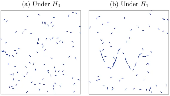
This paper is motivated by experiments in the field of Psychophysics (6) that study the ability of the Human Visual System at detecting curvilinear features in background clutter. In these experiments, human subjects are shown an image consisting of oriented small segments of same length dispersed in a square, such as in Figure 1.
(a) Under H0 (b) UnderH1
Figure 1: In Panel (a) we observe a realization under the null hypothesis (n = 100). In Panel (b) we observe a realization under the alternative hypothesis (n= 100, n1 = 40).
The locations and orientations of these segments are either purely random (panel (a)) or a curve is actually “hidden” among purely random clutter, which here means that a curve was used to simulate a fraction of the segments by randomly choosing segments that are tangent to the curve at their midpoint (panel (b)).
From a Statistics viewpoint, this detection task, that human subjects are asked to perform, can be formalized into a hypothesis testing problem.
We say that a curve γ ⊂ [0,1]2, parametrized by arclength, interpolates (z, w) ∈ [0,1]2 ×S1 if there is x such that γ(x) = z and ˙γ(x) = w, where S1 denotes the unit circle and ˙γ(x) the
derivative ofγ atx.
We observen segments of fixed length dispersed in the unit square.
• Under thenull hypothesis, the segments have locations and orientations sampled uniformly at random in [0,1]2×S1.
• Under the (composite) alternative hypothesis, the segments are as above except for n1 of them that are chosen among those that a fixed curve γ interpolates. The curve γ is unknown but restricted to belong to some known class Γ.
Note that we do not specify the distribution of the segments tangent to the curve.
Forγ ∈Γ, define
and, with some abuse of notation,
Nn→(Γ) = max
γ∈Γ N →
n (γ).
In (2), the test that rejects for large Nn→(Γ) was analyzed for Γ the class of curves in the unit square with length and curvature bounded by some constantc >0. In particular, it was shown that, under the null hypothesis, for some constants 0< A < B <∞,
PnA n1/4 ≤Nn→(Γ)≤B n1/4o→1, n→ ∞.
Note that the upper bound implies that this test is powerful whenn1 ≥Bn1/4.
A note on computing. The problem of computing Nn→(Γ) exactly can be reframed into the Reward-Budget Problemof (5), the same problem appearing with different names elsewhere, e.g. (3; 4). Problems of this flavor are all NP-hard, though in theory there are algorithms that run in polynomial time that compute good approximations (5).
In contrast, when Γ is the set of graphs of functions of the first coordinate (say), with first and second derivatives bounded by some constantsc1 andc2, a Dynamic Programming algorithm is available – see (8).
In this paper, we generalize this setting to higher dimensions. Let G(k, d) be the set of k
-dimensional linear subspaces inRd. ToG(k, d) we associate its uniform measureλ, which is the
only invariant probability measure onG(k, d) that is invariant under the action of the orthogonal
groupO(d) – see (10), Section 1.
For a functionf : [0,1]k→[0,1]d differentiable atx, let
~
f(x) = span{∂sf(x) :s= 1, . . . , k}.
A function f : [0,1]k → [0,1]d is said to interpolate (z, w) ∈ [0,1]d×G(k, d) if there exists
x∈[0,1]k such thatf(x) =z and f~(x) =w.
We consider the following hypothesis testing problem. We observe
{(Zi, Wi) :i= 1, . . . , n} ⊂[0,1]d×G(k, d).
• Under the null hypothesis, {(Zi, Wi) : i= 1, . . . , n} are independent and identically
uni-formly distributed in [0,1]d×G(k, d).
• Under the(composite) alternative hypothesis,{(Zi, Wi) :i= 1, . . . , n} are as above except
for n1 of them that are chosen among those that a fixed function f interpolates. The functionf is unknown but restricted to belong to some known classF.
Before specifying F, we introduce some notation. For a vector x = (x1, . . . , xd) ∈ Rd, the
supnorm is defined as kxk∞ = max{|xi| : i = 1, . . . , d}. For a function f : Ω ⊂ Rk → Rd,
byh·,·iandk · krespectively. The angle∠(H, K)∈[0, π] between two linear subspacesH, K⊂
Rd, with 1≤dimH ≤dimK, is defined by
∠(H, K) = max
u∈Hminv∈Karccos
hu, vi kukkvk
.
This corresponds to the largest canonical angle as defined in (7) and constitutes a metric on
G(k, d) – see also (1) for a related study of the largest canonical angle between two subspaces
uniformly distributed inG(k, d).
The class F, parametrized by β ≥ 1, is defined as the set of twice differentiable, one-to-one functionsf : [0,1]k →[0,1]d with the following additional properties:
• For alls= 1, . . . , k, 1/β ≤ k∂sf(x)k∞≤β for allx∈[0,1]k;
• For alls, t= 1, . . . , k,k∂stf(x)k∞≤β for all x∈[0,1]k;
• For alls= 1, . . . , k and x∈[0,1]k,
∠(∂sf(x),span{∂tf(x) :t6=s})≥
1 2β(d−k),
which is void ifk= 1. (In this paper, we identify a non-zero vector with the one dimensional linear subspace it generates.)
The last condition and the constraint β ≥ 1 ensure that F contains graphs of the form x → (x, g(x)), whereg: [0,1]k→[0,1]d−k satisfies the first two conditions – see Lemma 6.1.
Define
Nn→(f) = #{i= 1, . . . , n:f interpolates (Zi, Wi)},
and, with some abuse of notation,
Nn→(F) = max
f∈F N →
n (f).
Let
~
ρ= k
k+ (d−k)(k+ 2).
Theorem 1.1. There are finite, positive constantsA andB depending only onk, d, β such that, under the null hypothesis,
PnA n~ρ≤Nn→(F)≤B nρ~o→1, n→ ∞.
As before, this implies that the test that rejects for large values of Nn→(F) is powerful when n1> Bn~ρ.
2
Another Hypotheses Testing Problem
We introduce another hypothesis testing problem as a stepping stone towards proving Theorem 1.1 and also for its own sake.
Let α > 1, β > 0 and define r = ⌊α⌋ = max{m ∈ N :m < α}. (In this paper, we include 0
in N.) Define the H¨older class Hk,d(α, β) to be the set of functions f : [0,1]k → [0,1]d, with
f = (f1, . . . , fd) such that, for alls= (s1, . . . , sk)∈Nk with |s|=s1+· · ·+sk ≤r,
kf(s)(x)k∞≤β ∀x∈[0,1]k;
and, for alls∈Nk with |s|=r,
kf(s)(x)−f(s)(y)k∞≤βkx−yk∞α−r ∀x, y∈[0,1]k,
wheref(s) = (∂
s1···skf1, . . . , ∂s1···skfd). When there is no possible confusion, we use the notation
H= Hk,d−k(α, β).
Fixr0 an integer such that 1≤r0≤r. Let
S={s∈Nk :|s| ≤r0},
with cardinality
|S|=
r0
X
s=0
s+k−1 k−1
.
We denote by yS
a vector in R(d−k)|S| and by f(S)(x) the vector (f(s)(x) : s ∈S). A function f ∈ H is said to interpolate (x, yS
)∈[0,1]k×R(d−k)|S| iff(S)(x) =yS.
Consider the following hypothesis testing problem. We observe
{(Xi, YiS)) :i= 1, . . . , n} ⊂[0,1]k×R(d−k)| S|
.
• Under the null hypothesis, {(Xi, YiS) : i= 1, . . . , n} are independent and identically
uni-formly distributed in [0,1]k×[0,1]d−k×[−β, β](d−k)(|S|−1)
.
• Under the(composite) alternative hypothesis,{(Xi, YiS) :i= 1, . . . , n}are as above except
for n1 of them that are chosen among those that a fixed function f interpolates. The functionf is unknown but restricted to belong toH.
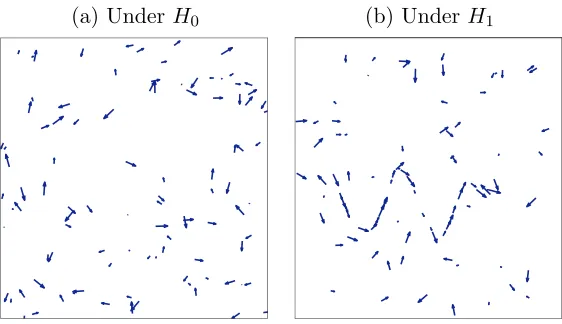
Figure 2 shows an example, with d= 2 andr0= 1. Define
Nn(r0)(f) = #{i= 1, . . . , n:f interpolates (Xi, YiS)},
and, with some abuse of notation,
Nn(r0)(H) = max
f∈HN
(a) Under H0 (b) UnderH1
Figure 2: In Panel (a) we observe a realization under the null hypothesis (n = 100). In Panel (b) we observe a realization under the alternative hypothesis (n= 100, n1 = 40).
Let
ρ(r0) =
k
k+α(d−k)w =
1
1 +α(d/k−1)w , where
w=
r0
X
s=0
(1−s/α)
s+k−1 k−1
.
Theorem 2.1. There are finite, positive constantsA andB depending only onk, d, α, β, r0 such that, under the null hypothesis,
PnA nρ(r0)≤Nn(r0)(H)≤B nρ(r0)o
→1, n→ ∞.
As before, this implies that the test that rejects for large values of Nn(r0)(H) is powerful when
n1> Bnρ(r0).
Remark. For α = 2 and r0 = 1, ρ(r0) = ρ~, meaning that Nn(r0)(H) and Nn→(F) are, in that
case, of same order of magnitude with high probability. This will be used explicitly in Section 6 when proving the lower bound in Theorem 1.1.
3
Proof of the upper bound in Theorem 2.1
ForyS
1, y2S∈R(d−k)|S|, define the discrepancy Φ(yS
1, y
S
2) = maxs ∈S ky
s
1−y
s
2kα/(α−|s|)
∞ .
The discrepancy Φ induces a discrepancy on functions, namely
Φ(f, g) = max
s∈S kf
(s)−g(s)kα/(α−|s|)
∞ .
Lemma 3.1. There is a constant c1 =c1(k, d, α, β, r0)>0 such that, for all ε >0,
logLε≤c1ε−k/α.
Lemma 3.1 follows immediately from the proof of Theorem XIII in (9), Chapter “ε-entropy and ε-capacity of sets in functional spaces”.
For a set K ⊂Rk×R(d−k)|S| and ε >0, we denote byKε,Φ the set of points (x, yS) such that
there is (x1, y1S)∈K withx1 =x and Φ(yS1, y
S
)≤ε.
For eachε, we select anε-net{fj :j= 1, . . . , Lε} of Hfor Φ. Forj= 1, . . . , Lε, we define
Kj = {(x, yS)∈Rk×R(d−k)|S|: Φ(yS, f( S)
j (x))≤ε}
= graphS(fj)ε,Φ,
where, for f ∈ H,
graphS(f) ={(x, f(S)(x)) :x∈[0,1]k} ⊂[0,1]k×R(d−k)|S|.
We extend N(r0)(·) to subsets K ⊂ Rk×R(d−k)|S|, by defining N(r0)(K) to be the number of points (Xi, YiS) that belong to K.
Let
Mn(ε) = max j=1,...,Lε
Nn(r0)(Kj).
By definition, it is straightforward to see that
Nn(r0)(H)≤Mn(ε),
for all ε >0. We therefore focus on bounding Mn(ε).
By Boole’s inequality, we have
P{Mn(ε)> b} ≤Lε· max j=1,...,Lε
PnNn(r0)(Kj)> b o
.
Moreover, we know that, for any setK ⊂Rk×R(d−k)|S|,
N(r0)
n (K)∽Bin(n, µ(K)),
whereµis the uniform measure on [0,1]k×[0,1]d−k×[−β, β](d−k)(|S|−1). Hence,
P{Mn(ε)> b} ≤ Lε· max j=1,...,Lε
P{Bin(n, µ(Kj))> b}
= Lε·P
Bin(n,max
j µ(Kj))> b
.
Lemma 3.2. There is c2 >0 such that, for all f ∈ H and all ε >0,
µ graphS
(f)ε,Φ
Proof of Lemma 3.2. Start with
graphS(f)ε,Φ⊂ ∪x∈[0,1]k {x}
O
s∈S
B(f(s)(x), ε1−|s|/α),
whereB(y, η) denotes the supnorm ball inRd−k centered aty of radiusη.
Hence, integrating overx∈[0,1]k last, we have
µ(graphS(f)ε,Φ)≤c2Y
s∈S
(ε1−|s|/α)d−k=c2 ε(d−k)w.
Using Lemma 3.2, we arrive at
P{Mn(ε)> b} ≤Lε·P n
Bin(n, c2ε(d−k)w)> bo.
Lemma 3.3. There is a constant c > 0 such that, for any n positive integer and p ∈(0,1/2), and for all b >2np,
P{Bin(n, p)> b} ≤exp(−c·b).
Lemma 3.3 follows directly from standard large deviations bounds for binomial random variables – see (12), p. 440, Inequality 1, (ii).
We use Lemma 3.3 to obtain
PnBin(n, c2ε(d−k)w)> bo≤exp(−c·b),
for all b >2nc2ε(d−k)w.
Collecting terms, we arrive at the following inequality, valid forB >2c2,
P
n
Mn(ε)> B ε(d−k)wn o
≤expc1ε−k/α−c3 B ε(d−k)wn
.
Choose ε= n−α/(k+α(d−k)w), so that ε−k/α =ε(d−k)wn=nρ(r0). Then, the result above trans-forms into
P
n
Mn(ε)> B nρ(r0) o
→0, n→ ∞,
valid forB >(c1/c3)∨2c2.
4
Proof of the lower bound in Theorem 2.1
We use the notations appearing in Section 4, except for the various constants which are refreshed in this section.
For each s ∈ S, take ψs : Rk → R infinitely differentiable, supported in [−1/2,1/2]k, and
satisfying ψs(t)(0) = 0 if t∈S and t6=s; and ψ( s)
s (0) = 1.
Letc1 ≥1 such thatc1 ≥ kψ(
t)
Again, choose ε > 0 such that ε−k/α = ε(d−k)wn. Define εs = ε1−|s|/α and, with c2 >1 to be
Fixm∈M. We have kh(j,mt)k∞=kg(j,mt)k∞ (ε′)−|t|, with
kg(j,mt)k∞≤Yi0(m),j X
0≤t′≤t
t t′
kψ(0t′)k∞ X
s∈S
(ε′)|s| Y
s i(m),j
Y0 i(m),j
kψ(st−t′)k∞.
Since Y0
i(m),j ≤εand
0≤(ε′)|s| Y
s i(m),j
Y0 i(m),j
≤2c|2s|/α ≤2cr/α2 ,
we have, for |t| ≤r+ 1, kgj,m(t)k∞≤c3 cr/α2 ε, withc3 =c3(α, k)>0. In particular,c3 does not depend on the choice of c2. Choose c2>1 such thatc3 cr/α2 −1≤β.
Hence, for all tsuch that |t| ≤r+ 1,
kh(j,mt)k∞≤c3 cr/α2 ε(ε′)−|
t|
=c3 c(r−|
t|)/α
2 ε1−|
t|/α
.
This implies that, for εsmall enough,hj takes values in [0,1] and
kh(jt)k∞≤β,
for all tsuch that |t| ≤r.
Remains to prove that, for allt such that|t|=r,
|h(jt)(x′)−h(jt)(x)| ≤βkx′−xkα∞−r,
for all x, x′∈[0,1]k.
• Supposekx′−xk∞> ε′;
|h(jt)(x′)−hj(t)(x)| ≤ kh(jt)k∞ ≤ c3 cr/α2 ε(ε′)−r
≤ c3 cr/α2 ε(ε′)−r(kx−x′k∞/ε′)α−r ≤ c3 cr/α2 −1 kx−x′kα∞−r.
• Supposekx−x′k∞≤ε′ and lett+ = (t1+ 1, . . . , tk);
|h(jt)(x′)−hj(t)(x)| ≤ khj(t+)k∞kx−x′k∞
≤ c3 cr/α2 ε(ε′)−(r+1)·(ε′)1−(α−r)kx−x′kα∞−r = c3 cr/α2 −1 kx−x′kα∞−r.
5
Proof of the upper bound in Theorem 1.1
Let Ψ be the discrepancy onRd×G(k, d) defined by
Ψ((z, H),(z1, H1)) = max{kz−z1k∞,∠(H, H1)2}.
Each f ∈ F is identified with (f, ~f), viewed as a function on [0,1]k with values in Rd×G(k, d)
– the first and third constraints on the derivatives of f ∈ F guarantee that f~(x) is indeed a k-dimensional subspace ofRdfor allx∈[0,1]k. With this perspective, Ψ induces a discrepancy
on F. The proof is based on coverings of F with respect to that discrepancy – still denoted by Ψ.
It turns out that Ψ is dominated by the discrepancy Φ defined in Section 4, with α = 2 and r0 = 1. Indeed, we have the following.
Lemma 5.1. There is a constant c=c(k, d, β) such that, for any f, g∈ F andx∈[0,1]k,
∠f~(x), ~g(x)≤c max
s=1,...,kk∂sf(x)−∂sg(x)k∞.
To get Lemma 5.1, we apply Lemma D.1 in Appendix D with ui (resp. vi) defined as ∂if(x)
(resp. ∂ig(x)) andc1 = 1/β,c2=β,c3= 1/(2β(d−k)).
Therefore, theε-covering number ofF with respect to Ψ is bounded by the ε-covering number ofF with respect to Φ, whose logarithm is of orderε−k/2 – see Lemma 3.1, where denters only in the constant.
Following the steps in Section 4, we only need to find an equivalent of Lemma 3.2, namely compute an upper bound on the measure of theε-neighborhood of
{(f(x), ~f(x)) :x∈[0,1]k} ⊂Rd×G(k, d)
for the discrepancy Ψ, valid for all f ∈ F. ForH∈G(k, d), let
B(H, ε) ={K ∈G(k, d) :∠(H, K)≤ε}.
As in the proof of Lemma 3.2, we are left with computing a upper bound onλ(B(H, ε)), which is independent ofH ∈G(k, d) sinceλis invariant under the (transitive) action of the orthogonal
group. (Remember thatλdenotes the uniform measure onG(k, d).)
Lemma 5.2. There is a constant c =c(k, d) such that, for all ε > 0 and for all H ∈ G(k, d),
λ(B(H, ε))≤c ε(d−k)k.
Lemma 5.2 is a direct consequence of Lemma B.1 in Appendix B and the fact thatλ(G(k, d)) = 1.
6
Proof of the lower bound in Theorem 1.1
Lemma 6.1. For all g∈ H, the functionf(x) = (x, g(x))belongs to F.
Lemma 6.1 is proved in Appendix C.
Let W be sampled uniformly at random in G(k, d). With probability one, there is a unique
set of vectors in Rd−k, {Ys
: |s| = 1}, such that W = span{(s, Ys
) :|s|= 1}. Indeed, W has the same distribution as span{w1, . . . , wk}, where w1, . . . , wk are i.i.d. uniformly distributed
on the unit sphere of Rd and therefore, with probability one, hwi, eii 6= 0 for all i = 1, . . . , k,
{ei :i= 1, . . . , d} being the canonical basis of Rd. The uniqueness comes from the fact that a
subspace of the form span{(s, Ys
) :|s|= 1} does not contain a vector of the form (0, Y), with Y ∈Rd−k\ {0}, so it does not contain two distinct vectors of the form (s, Y1) and (s, Y2).
Through the mapκthat associatesW to{Ys
:|s|= 1}, the uniform measure onG(k, d) induces
a probability measureν on R(d−k)k. If we observe{(Zi, Wi) :i= 1, . . . , n}, we let
Zi = (Xi, Yi)∈Rk×Rd−k and Wi = span{(s, Yis) :|s|= 1}.
With here S ={s ∈ Nk : |s| ≤ 1}, we thus obtain {(Xi, YS
i ) :i = 1, . . . , n}, independent and
with common distribution Λk⊗Λd−k⊗ν ≡Λd⊗ν, where Λℓ is the uniform measure on [0,1]ℓ.
Note that, if g ∈ H interpolates {(Xi, YiS) : i = 1, . . . , n}, then f defined by f(x) = (x, g(x))
belongs to F by Lemma 6.1 and interpolates {(Zi, Wi) : i = 1, . . . , n}. With Λd⊗ν playing
the role of µ, the uniform measure on [0,1]k×[0,1]d−k×[−β, β](d−k)(|S|−1), the present setting parallels the situation in Section 4. Following the arguments given there, we are only left with obtaining the equivalent of Lemma 4.1. Looking at the proof of Lemma 4.1 in Section A, all we need is a lower bound of the form
Λd⊗ν(R0)≥c µ(R0) =c (ε′)kε(d−k)w =c εk/2+(d−k)(1+k/2).
(Hereα= 2 and w= 1 +k/2.) Because
Λd⊗ν(R0) =c εk/2+(d−k)·ν
[0, ε1/2](d−k)k,
the following lemma provides what we need.
Lemma 6.2. There is a constant c=c(k, d)>0 such that, for all ε >0 small enough,
ν[0, ε](d−k)k> c ε(d−k)k.
To prove Lemma 6.2, we first show that for some constant c = c(k, d) > 0, κ−1([0, ε](d−k)k)
contains B(H, c ε), where H = span{e1, . . . , ek} and {e1, . . . , ed} is the canonical basis of Rd.
Indeed, letc be the constant provided by Lemma D.2 and considerK∈B(H, c ε). Let κ(K) = {y1, . . . , yk}, so that K = span
ei+yi:i= 1, . . . , k . Applying Lemma D.2 with ui = ei for
i = 1, . . . , k, v = ej +yj and uk+1 = (v−P v)/kv−P vk∞, where P denotes the orthogonal projection ontoH, we get that∠(v, H)≥ckv−P vk∞. Withkv−P vk∞=kyjk∞ and the fact that ∠(v, H) ≤ ∠(K, H), we see that we have kyjk∞ ≤ ε. This being true for all j, we have
κ(K)∈[0, ε]k(d−k). We then apply the following result.
Lemma 6.3. There is a constantc=c(k, d)>0such that, for allε >0and for allH∈G(k, d),
Lemma 6.3 is a direct consequence of Lemma B.2 in Appendix B and again the fact that λ(G(k, d)) = 1.
Appendix
A
Proof of Lemma 4.1
Lemma 4.1 is a conditional version of The Coupon Collector’s Problem – see e.g. (11). We nevertheless provide here an elementary proof.
Let K = N(r0)
n (∪m∈M Rm). We know that K ∼Bin(n, p), where p =|M| µ(R0) with |M| ∝
nρ(r0) and
µ(R0) = (ε′)k·(ε/2)d−k· Y
s∈S\{0}
(ε|s|/(2β))d−k ∝(ε′)kε(d−k)w.
This implies that pn = c′|M| for some c′ > 0 not depending on n, by definition of ε and ε′. Letc =c′/2 and c0 ∈(e−c,1), and also, to simplify notation, letℓ=|M| and S =|M| − |M|. Because|M| ∝nρ(r0), it is enough to show thatP{S > c0 ℓ} →0 asn→ ∞.
We have
P{S > c0 ℓ} ≤P{S > c0 ℓ|K > c ℓ}+P{K > c ℓ}, withP{K > c ℓ} →0 asn→ ∞ by Lemma 3.3, and
P{S > c0 ℓ|K > c ℓ} ≤P{S > c0 ℓ|K=⌈c ℓ⌉}. Using Chebychev’s inequality, we get
P{S > c0 ℓ|K =⌈c ℓ⌉} ≤
var{S|K=⌈c ℓ⌉} (c0 ℓ−E{S|K=⌈c ℓ⌉})2. We know that for any non-negative integerk,
E{S|K =k}=ℓ(1−1/ℓ)k, and
var{S|K=k}=ℓ((1−1/ℓ)k−(1−1/ℓ)2k) +ℓ(ℓ−1)((1−2/ℓ)k−(1−1/ℓ)2k). Therefore, whenℓ→ ∞,
E{S|K =⌈c ℓ⌉}∽e−cℓ, and, for allℓ,
var{S|K =⌈c ℓ⌉} ≤c1ℓ, so that, when ℓis large,
var{S|K=⌈c ℓ⌉} (c0 ℓ−E{S|K=⌈c ℓ⌉})2 ≤
c2 ℓ.
Since ℓis an increasing function ofnthat tends to infinity, we conclude that
B
Coverings of
G
(
k, d
)
Lemma B.1. There is a constantc=c(k, d)>0such that, for all ε >0, there isH1, . . . , Hℓ∈
G(k, d) with ℓ > c ε−(d−k)k and B(Hi, ε)∩B(Hj, ε) =∅ if i6=j.
Proof of Lemma B.1. Fixε >0 and consider
Hn= span v = v1. It is straightforward to see that the conditions are satisfied, since in particular v1 = u1+kv1−u1k∞uk+1. Hence, for a constantc >0 depending only on k, d, given by Lemma D.4. As in the proof of Lemma B.1, define
Furthermore,
arccos
s
(d−k)β2 1 + (d−k)β2
!
= arctan
1 β√d−k
≥ 1
2β√d−k,
where the last inequality comes from the fact that arctan(y)≥y/2 for y≤π/2.
D
Auxiliary Results in Euclidean Spaces
Lemma D.1. Let c1, c2, c3 be three positive constants. Let u1, . . . , uk;v1, . . . , vk ∈Rd such that
for alli= 1, . . . , k, c1 ≤ kvik∞,kuik∞≤c2, and, ifk≥2,
∠(ui,span{uj :j6=i})≥c3;
∠(vi,span{vj :j 6=i})≥c3. Then, for a constant c depending only on k, d, c1, c2, c3,
∠(span{ui :i= 1, . . . , k},span{vi :i= 1, . . . , k})≤c max
i=1,...,kkvi−uik∞.
Proof of Lemma D.1. By multiplying the constants that appear in the Lemma by constants that depend only ond, we can assume that the conditions in the Lemma hold for the Euclidean norm. Throughout, letε= maxi=1,...,kkvi−uik∞.
First assume that u1, . . . , uk (resp. v1, . . . , vk) are orthonormal. Take
u=X
i
ξiui ∈span{ui :i= 1, . . . , k},
of norm equal to 1. Define
v=X
i
ξivi∈span{vi :i= 1, . . . , k}.
We show that
arccos(|hu, vi|) =O(ε), by showing that
hu, vi= 1 +O(ε2). This comes from the fact that, sincekuk=kvk= 1,
hu, vi= 1− ku−vk2/2,
and
ku−vk ≤X
i
|ξi| kui−vik ≤
If u1, . . . , uk (resp. v1, . . . , vk) are not orthonormal, we make them so. Define a′1 = u1 and a1=a′1/ka′1k, and for i= 2, . . . , k, define
a′i =ui− i−1
X
j=1
hui, ajiaj,
and ai =a′i/ka′ik. Similarly, define b′1 =v1 and b1 =b′1/kb′1k, and for i= 2, . . . , k, define
b′i =vi− i−1
X
j=1
hvi, bjibj,
and bi=b′i/kb′ik.
We have, fori= 1, . . . , k,c1sinc3 ≤ ka′ik ≤c2. Indeed, sincea′i is the difference betweenui and
its orthogonal projection onto span{u1, . . . , ui−1}, it follows that
ka′ik=kuik sin∠(ui,span{u1, . . . , ui−1}),
with
∠(ui,span{u1, . . . , ui−1})≥∠(ui,span{uj :j6=i})≥c3>0. In the same way, for i= 1, . . . , k,c1sinc3≤ kb′ik ≤c2.
We also have a′i−b′i = O(ε). We prove that recursively. First, ka′1 −b′1k = ku1 −v1k ≤ ε. Assumea′
i−1−b′i−1=O(ε). This impliesai−1−bi−1=O(ε); indeed,
ai−1−bi−1 = k
b′i−1ka′i−1− ka′i−1kb′i−1 ka′
i−1kkb′i−1k ≤ (ka
′
i−1k+O(ε))a′i−1− ka′i−1k(a′i−1+O(ε)) c2
= O(ε).
Now,
a′i−b′i=ui−vi−(hui, ai−1iai−1− hvi, bi−1ibi−1), withui−vi =O(ε) and
hvi, bi−1ibi−1 =hvi, ai−1+O(ε)i(ai−1+O(ε)) =hvi, ai−1iai−1+O(ε). So that
hui, ai−1iai−1− hvi, bi−1ibi−1 =hui−vi, ai−1iai−1+O(ε) =O(ε). Hence, the recursion is satisfied.
We then apply the first part to a1, . . . , ak and b1, . . . , bk.
Lemma D.2. Fix c1, c2, c3 three positive constants. Let u1, . . . , uk+1 ∈ Rd such that for i = 1, . . . , k+ 1,c1≤ kuik∞≤c2, and
∠(ui,span{uj :j6=i})≥c3.
Then, there is a positive constantcdepending only on k, d, c1, c2, c3 such that, for allv=Piξiui
withkvk∞≤c2,
Proof of Lemma D.2. The proof is similar to that of Lemma D.1 above. Again, we may work with the Euclidean norm instead of the supnorm.
First assume thatu1, . . . , uk+1are orthonormal. Takev =Piξiuiof norm equal to atk. Without loss of generality, we may assume that
|hui, eii| ≥c(k−1, d), ∀i= 1, . . . , k−1.
Conclude by calling the right handsidec3 and letting
Lemma D.4. Let e1, . . . , ed be the canonical basis of Rd. There is a constant c =c(k, d) >0
such that, for u1, . . . , uk any orthonormal set of vectors in Rd, there exists a permutation σ of
{1, . . . , d}, such that
span{u1, . . . , uk}= span
eσ(1)+v1, . . . , eσ(k)+vk ,
where, for all i= 1, . . . , k,
vi ∈span{eσ(j) :j=k+ 1, . . . , d},
and kvik∞≤c.
Proof of Lemma D.4. Applying Lemma D.3, there isc1>0 and a permutation σ such that
|hui, eσ(i)i| ≥c1, ∀i= 1, . . . , k.
Without loss of generality, supposeσ = id.
We now triangulate the matrix with column vectors u1, . . . , uk. In other words, we consider
{u′i :i= 1, . . . , k}, where u′i is the orthogonal projection of ui onto span{ei, ek+1, . . . , ed}. For
all i = 1, . . . , k, we have u′
i = ξiei +wi, where |ξi| ≥ c1 and wi ∈ span{ek+1, . . . , ed} with
kwik∞≤1. Define vi=wi/ξi and conclude with the fact that
span
u′1, . . . , u′k = span{u1, . . . , uk}.
References
[1] P.-A. Absil, A. Edelman, and P. Koev. On the largest principal angle between random subspaces. Linear Algebra Appl., 414 (2006), no. 1, 288–294. MR2209246
[2] E. Arias-Castro, D. L. Donoho, X. Huo, and C. Tovey. Connect-the-dots: How many random points can a regular curve pass through? Adv. in Appl. Probab., 37 (2005), no. 3, 571–603. MR2156550
[3] E. Arkin, J. Mitchell, and G. Narasimhan. Resource-constrained geometric network opti-mization. In Proc. of ACM Symposium on Computational Geometry, Minneapolis, (1997), 307–316.
[4] B. Awerbuch, Y. Azar, A. Blum, and S. Vempala. New approximation guarantees for minimum-weightk-trees and prize-collecting salesmen. SIAM J. Comput., 28 (1999), no. 1, 254–262. MR1630453
[5] B. DasGupta, J. Hespanha, and E. Sontag. Computational complexities of honey-pot search-ing with local sensory information. In 2004 American Control Conference (ACC 2004), pages 2134–2138. 2004.
[7] G. H. Golub and C. F. Van Loan. Matrix computations. Johns Hopkins Studies in the Mathematical Sciences. Johns Hopkins University Press, Baltimore, MD, third edition, 1996. MR1417720
[8] X. Huo, D. Donoho, C. Tovey, and E. Arias-Castro. Dynamic programming methods for ‘connecting the dots’ in scattered point clouds. INFORMS J. Comput., 2005. To appear.
[9] A. N. Kolmogorov.Selected works of A. N. Kolmogorov. Vol. III, volume 27 ofMathematics and its Applications (Soviet Series). Kluwer Academic Publishers Group, Dordrecht, 1993. MR1228446
[10] V. D. Milman and G. Schechtman. Asymptotic theory of finite-dimensional normed spaces, volume 1200 of Lecture Notes in Mathematics. Springer-Verlag, Berlin, 1986. With an appendix by M. Gromov. MR856576
[11] F. Mosteller. Fifty challenging problems in probability with solutions. Addison-Wesley Publishing Co., Inc., Reading, Mass.-London, 1965. MR397810