This ar t icle was dow nloaded by: [ Univer sit as Dian Nuswant or o] , [ Rir ih Dian Prat iw i SE Msi] On: 29 Sept em ber 2013, At : 20: 11
Publisher : Rout ledge
I nfor m a Lt d Regist er ed in England and Wales Regist er ed Num ber : 1072954 Regist er ed office: Mor t im er House, 37- 41 Mor t im er St r eet , London W1T 3JH, UK
Accounting and Business Research
Publ icat ion det ail s, incl uding inst ruct ions f or aut hors and subscript ion inf ormat ion: ht t p: / / www. t andf onl ine. com/ l oi/ rabr20
Does graph disclosure bias reduce the cost of equity
capital?
Fl ora Muiño a & Marco Trombet t a b a
Depart ament o de Economía de l a Empresa, Universidad Carl os III de Madrid b
Depart ment of Account ing and Management Cont rol , Inst it ut o de Empresa Business School , Cal l e Pinar 15 – 1B, Madrid, 28006, Spain Phone: +34 917451369 Fax: +34 917451369 E-mail : Publ ished onl ine: 04 Jan 2011.
To cite this article: Fl ora Muiño & Marco Trombet t a (2009) Does graph discl osure bias reduce t he cost of equit y capit al ?, Account ing and Business Research, 39: 2, 83-102, DOI: 10. 1080/ 00014788. 2009. 9663351
To link to this article: ht t p: / / dx. doi. org/ 10. 1080/ 00014788. 2009. 9663351
PLEASE SCROLL DOWN FOR ARTI CLE
Taylor & Francis m akes ever y effor t t o ensur e t he accuracy of all t he infor m at ion ( t he “ Cont ent ” ) cont ained in t he publicat ions on our plat for m . How ever, Taylor & Francis, our agent s, and our licensor s m ake no
r epr esent at ions or war rant ies w hat soever as t o t he accuracy, com plet eness, or suit abilit y for any pur pose of t he Cont ent . Any opinions and view s expr essed in t his publicat ion ar e t he opinions and view s of t he aut hor s, and ar e not t he view s of or endor sed by Taylor & Francis. The accuracy of t he Cont ent should not be r elied upon and should be independent ly ver ified w it h pr im ar y sour ces of infor m at ion. Taylor and Francis shall not be liable for any losses, act ions, claim s, pr oceedings, dem ands, cost s, expenses, dam ages, and ot her liabilit ies w hat soever or how soever caused ar ising dir ect ly or indir ect ly in connect ion w it h, in r elat ion t o or ar ising out of t he use of t he Cont ent .
This ar t icle m ay be used for r esear ch, t eaching, and pr ivat e st udy pur poses. Any subst ant ial or syst em at ic r epr oduct ion, r edist r ibut ion, r eselling, loan, sub- licensing, syst em at ic supply, or dist r ibut ion in any
1. Introduction
Prior research on graph usage in annual reports has documented two important facts. First, graph usage increases when company performance im-proves (e.g. Steinbart, 1989 and Beattie and Jones, 1992). Second, an important proportion of graphs are distorted to portray a more favourable view of the company than reflected in the financial state-ments (e.g. Beattie and Jones, 1999 and Mather et al., 1996). Thus, the existing literature supports the notion that managers use distorted graphs to man-age the impression created in the perceptions of users of annual reports1 (e.g. Beattie and Jones, 2000). However, Beattie and Jones (2008: 22), after reviewing the existing literature on graph usage in annual reports, conclude:
‘A fundamental issue to be addressed by future research is whether an impact on a user’s percep-tions of the organisation carries through to an impact on their decision. For example, are in-vestment decisions affected by graphical presen-tation choices? We need, therefore, to carry out research into the effect, if any, of financial graphs on analysts’ earnings forecasts, stock prices and the relationship decisions of other key stakeholder groups such as employees, cus-tomers and suppliers’
From a theoretical point of view, the potential ef-fect of graph distortion on the functioning of the stock market is a controversial issue. On the one hand, the literature on ‘herding’ and ‘limited atten-tion’ in financial markets shows that economic agents may neglect a considerable part of their private information because of reputation and co-ordination effects or information processing limi-tations.2Consequently, graphs can have an impact on users’ judgments and decisions, even when the information represented in graphs can be gathered also in other parts of the annual report. On the other hand, the efficient markets hypothesis (EMH) tells us that prices should include all the publicly available information. Hence, graph dis-tortion should not affect prices because they should be based on all the information available on
Does graph disclosure bias reduce the cost
of equity capital?
Flora Muiño and Marco Trombetta*
Abstract—Firms widely use graphs in their financial reports. In this respect, prior research demonstrates that com-panies use graphs to provide a favourable outlook of performance, suggesting that they try to manage the impres-sion created in users’ perceptions. This study tests whether by means of distorted graphs managers are able to influence users’ decisions in the capital market. By focusing on the effects of distorted graphs on the cost of equi-ty capital, we provide preliminary evidence on one of the possible economic consequences of graph usage. The re-sults of this investigation suggest that graph disclosure bias has a significant, but temporary, effect on the cost of equity. Moreover, our results highlight the important role played by the overall level of disclosure as a condition-ing factor in the relationship between graphs and the cost of equity. Consequently, the results of the current study enhance our understanding of the complex interactions that take place in the stock market between information, in-formation intermediaries and investors.
Keywords: cost of equity, disclosure, graph distortion
*Flora Muiño is at the Departamento de Economía de la Empresa, Universidad Carlos III de Madrid and Marco Trombetta is at the Instituto de Empresa Business School, Madrid.
The authors would like to acknowledge the financial sup-port of the Spanish Ministry of Education through grants SEJ2004-08176-C02-02 and SEJ2007-67582-CO2-01/02. They appreciate the invaluable comments of the editor, two anonymous referees and from Salvador Carmona, Juan Manuel Garcia Lara, Miles Gietzmann, Manuel Illueca, Giovanna Michelon, Tashfeen Sohail, seminar participants at Universidad Carlos III (Madrid – Spain), Instituto de Empresa (Madrid – Spain), University of Padova (Italy), participants of the 29th annual EAA meeting (Dublin – Ireland) and partici-pants to the 5th Workshop on Empirical Research in Financial Accounting (Madrid – Spain). All remaining errors are the authors’ responsibility only.
Correspondence should be addressed to: Prof. Marco Trombetta, Instituto de Empresa Business School, Department of Accounting and Management Control, Calle Pinar 15 – 1B, 28006, Madrid (Spain). Tel: +34 917451369. Fax: +34 917451376. E-mail: [email protected].
This paper was accepted for publication in November 2008.
1Impression management techniques in annual reports are
not limited to the use and distortion of graphs. Extant research provides evidence consistent with the use of narratives as an impression management technique (e.g. Clatworthy and Jones, 2003; Aerts, 2005).
2A more detailed review of this literature is provided in the
next section of the paper.
the annual report and not only on the image por-trayed by graphs. Our aim is to provide empirical evidence that improves our understanding of this controversial issue and take a step forward in the direction indicated by Beattie and Jones (2008).
As an indicator of the capital market effects of graph distortion we use the cost of equity capital, measured both on an ex-ante (i.e. expected) and an ex-post (i.e. realised) basis.3The ex-ante measure is based on analysts’ forecasts of earnings issued at a certain point in time, soon after the publication of the annual report. This measure depends direct-ly on the expectations of those anadirect-lysts following the company at the time forecasts are issued. Based on the evidence provided by literature on herding and limited attention, we hypothesise that these expectations can be biased because of dis-torted graphs included in annual reports. However, on the grounds of the EMH, we do not expect graph distortion to affect our ex-post measure of the cost of equity, realised returns. Since realised returns aggregate the decisions taken by investors over a relatively large period of time (one year), we expect that the potential bias in analysts’ per-ceptions is corrected in the market by means of the aggregation process and the passing of time that allows new information to be impounded in stock prices.4
We base our analysis on a sample of Spanish companies quoted in the Madrid Stock Exchange (MSE) between 1996 and 2002. As compared to the US or the UK, where most prior studies on graphs have been developed, Spain has still a rela-tively underdeveloped capital market, where levels of corporate transparency are generally low.5 Moreover, prior research documents the existence of a higher level of herding in Spain than in coun-tries with more developed capital markets.6 If graph distortion is able to bias the perceptions of market participants, that is more likely to be ob-served in those markets, such as the MSE, with low corporate transparency and high levels of herding. When comparing US and European stock markets (excluding the UK), Bagella et al. (2007) find that the absolute bias in earnings forecasts is significantly higher in Europe than in the US. This is why we believe that the MSE is well suited to investigate whether graph distortion affects per-ceptions and decisions of market participants.
After controlling for other possible determinants of the cost of equity, we detect a significant nega-tive effect of favourable graph distortion on our ex-ante measure of the cost of equity. This effect is moderated by the overall level of disclosure so that, at high levels of transparency, the relationship between graph distortion and the ex-ante cost of equity becomes positive. However, when we turn to the ex-post analysis, we do not find any signifi-cant effect of graph distortion on realised returns.
We interpret this result as evidence that the effect on the ex-ante cost of equity is only temporary and confined to expectations. It is really an effect on the bias of the analysts’ forecasts that are used to calculate the ex-ante measure of the cost of equity. However, with the passing of time the aggregation process performed in the market corrects this bias. Our contribution to the literature is twofold. First, to the best of our knowledge, we are the first to provide empirical evidence on the capital mar-ket effects of graph distortion for quoted firms. Graph distortion is an ideal item from which to study the economic effects of impression manage-ment techniques. As stated by Merkl-Davies and Brennan (2007), the study of these effects is com-plicated by the difficulty of separating impression management (opportunistic distortion of informa-tion) from incremental information (provision of useful additional information). However, graph distortion, as an impression management tech-nique, is not affected by this problem. Given that the information portrayed in graphs is always available in another format in the same annual re-port, we can assume that distorted graphs are pure impression management tools and do not provide any incremental information.
Second, we provide additional evidence that supports the necessity of distinguishing between estimations by individuals and aggregated market behaviour, when studying the capital market ef-fects of impression management techniques. Short-term effects on individuals’ predictions can be corrected with the passing of time by the aggre-gation role played by market activity, so that they do not have an impact on long-window stock re-turns.
The structure of the paper is as follows. In the next section we review the existing literature and develop our research hypotheses. In Section 3 we describe our sample and the variables that we use in our empirical analysis. Section 4 contains the
3A review of the issues involved in the empirical
measure-ment of the cost of equity capital can be found, for example, in Botosan (2006).
4Temporary differences between ex-ante and ex-post
meas-ures of the cost of equity are depicted in Figure 1 and dis-cussed in detail in section 3.2.1.
5According to the World Federation of Exchanges, in 2002,
the latest year covered in our analysis, total value of share trad-ing in the MSE was $653,221m as compared to $4,001,340m for the London Stock Exchange or $10,310,055m for the New York Stock Exchange. Additionally, La Porta et al. (2006) pro-vide epro-vidence showing that the MSE has a lower index of dis-closure requirements (0.50, as compared to 0.83 and 1.00 for the UK and the US, respectively) and public enforcement (0.33 as compared to 0.68 and 0.90 for the UK and the US, re-spectively) .
6Ferruz Agudo et al. (2008) report a level of herding of
13.26% for Spain, a figure similar to that observed by Lobao and Serra (2002) for Portugal, but much higher than the 2% found by Lakonishok et al. (1992) for the US or the 3.3% ob-served by Wylie (2005) in the UK.
main results of our analysis. Section 5 summarises the analysis, provides some conclusions and draws implications.
2. Background and hypotheses
development
The importance of information for the functioning of the stock market is manifest. The whole notion of market efficiency in its different forms is based on how agents in the market react to information and how information is eventually reflected into prices. Graphs included in annual reports do not provide additional information, but they are a ve-hicle of information dissemination that makes data more visible and, when properly constructed, fa-cilitates its processing (Beattie and Jones, 1992). Extant research, however, shows that a significant proportion of graphs included by companies in their annual reports is materially distorted, gener-ally to portray corporate performance more favourably7 (e.g. Mather et al., 1996; Beattie and Jones, 1999). Researchers conclude that managers use distorted graphs to manage users’ perceptions (e.g. Beattie and Jones, 2000).
Experimental research provides evidence consis-tent with this conclusion. Taylor and Anderson (1986), Beattie and Jones (2002) and Arunachalam et al. (2002) all provide evidence that users’ per-ceptions are far more favourable when they are based on graphs that are favourably distorted. Arunachalam et al. (2002) explain this phenome-non on the basis of two findings of psychological research. First, Payne et al. (1993) show that peo-ple minimise their cognitive effort in order to achieve a certain level of accuracy. Second, Ricketts (1990) finds that people have difficulty at detecting presentation errors. Distorted graphs usually do not reverse or fundamentally change the reality as expressed by the data.
Participants’ perceptions are affected by distort-ed graphs even when the accurate numeric values are displayed as variable labels in graphs (e.g. Arunachalam et al., 2002). This suggests that par-ticipants focus their attention on the image por-trayed in graphs and ignore the numeric values. The fact that participants in these experimental studies neglect relevant information could be at-tributed to their low level of experience (they were students). However, extant research provides
evi-dence showing that even sophisticated users (ana-lysts) do not always make use of all available in-formation.
A substantial body of research in theoretical finance demonstrates that, under certain circum-stances, analysts may ignore a significant propor-tion of their private informapropor-tion. Trueman (1994) demonstrates that analysts tend to release forecasts similar to those reported by other analysts, even when their private information does not justify such forecasts. Similarly, Morris and Shin (2002) analyse the role of public information in contests where an agent needs to co-ordinate with other agents in order to maximise his/her payoff.8They show that, in these settings, it can be socially opti-mal to adopt coarser information systems instead of finer information systems. These theoretical predictions have been confirmed empirically. Stickel (1992), Graham (1999), Hong et al. (2000), and Welch (2000) provide evidence of analysts’ herding behaviour and Anctil et al. (2004) use an experimental setting to document the negative so-cial effects of a lack of coordination.
Literature on limited attention provides empiri-cal evidence showing that investors ignore valu-able information when making investment decisions. For instance, Doyle et al. (2003) find that the stock market does not fully appreciate the predictive power of expenses excluded from pro-forma earnings. Similarly, Hirshleifer et al. (2004) demonstrate that investors do not optimally use the information conveyed by net operating assets when assessing the sustainability of corporate per-formance. Furthermore, experimental studies such as those by Hopkins (1996), Hirst and Hopkins (1998) and Hirst et al. (2004) show that analysts’ judgments and valuations are affected by the income-measurement method (recognition versus disclosure in the footnotes) or the classification of items in the financial statements. These studies provide further evidence showing that even ex-perts ignore relevant information when making estimations and valuations; otherwise their valua-tions would not be affected by classification of in-formation in financial statements. Overall, prior research indicates that users tend to focus their at-tention on the most salient and easily processed in-formation, neglecting relevant data. This is attributed to limited attention and cognitive pro-cessing power (Hirshleifer and Teoh, 2003).
Graphs represent a prominent piece of informa-tion in the annual report and the informainforma-tion they convey can be processed by users fairly easily. Then, on the basis of both the theoretical argu-ments and the empirical and experimental evidence provided by extant literature, we hypothesise that market expectations and analysts’ estimations can be affected by favourable graph distortion, despite the fact that accurate values of the variables
dis-7Distortion refers to violations of what Tufte (1983) states
as an essential principle in graph construction: physical meas-ures on the surface of the graph should be directly proportion-al to the numericproportion-al quantities represented. The use of non-zero axis, broken axis, or non-arithmetic scales leads to graphs where equal distances along the axis do not represent equal amounts, that is, physical measures are not proportional to the underlying numerical values.
8The stock market is used by Morris and Shin (2002) as an
example of such a contest.
played in graphs are reflected in the financial state-ments. The ex-ante (expected) measures of the cost of equity capital depend directly on these ex-pectations and estimations in the sense that more optimistic forecasts about the future of the compa-ny are associated with a lower level of the ex-ante cost of capital. Hence, we state the following hy-pothesis to be tested in our study:
H1: Favourable graph distortion is negatively related to the ex-ante cost of equity capital. Disclosure and time are two additional factors that can affect the relationship between graph tortion and the cost of equity capital. Next, we dis-cuss the moderating effect that can be exercised by disclosure and afterwards we analyse the role played by the passing of time in correcting biases in ex-ante expectations.
The above-mentioned prior experimental re-search indicates that users have difficulties in de-tecting graph distortion. Corporate disclosure can ameliorate this situation by providing users with additional data that may turn out to be important clues in identifying distorted graphs.9Take, for ex-ample, the case of a firm presenting a slight in-crease in net sales, which is magnified in a distorted graph so that it appears as a strong rising trend. Distortion is difficult to detect because the direction of the change depicted graphically is the same as that shown by data in financial statements. However, if this firm provides operating data showing a decrease in production, readers are more likely to realise the graph is distorted. The role played by disclosure in correcting mispercep-tions is documented in the literature. Schrand and Walther (2000) observe that the bias introduced by strategic choices of prior-period benchmarks in earnings announcements is eliminated when the fi-nancial statements are released. Along the same line, in a controlled experiment, Krische (2005) finds that clear and quantitative information about prior-period transitory gains or losses allows par-ticipants to adjust the comparative prior period-earnings stated as a benchmark in period-earnings announcements. Based on prior evidence we ex-pect that the likelihood of distortion being detect-ed is increasing in the level of disclosure.
Detection of graph distortion can have an impact on users’ decisions because of the impairment in corporate disclosure credibility. As stated by Schmid (1992), graph distortion threatens the credibility of the entire report containing such a graphic. Therefore, when distortion is detected, users may perceive a higher risk associated with their decisions.10Theoretical studies by Easley and O’Hara (2004) and Leuz and Verrecchia (2005) predict the existence of a negative relationship be-tween the quality of information and the risk pre-mium required by investors. Easley and O’Hara
(2004) show that information precision reduces the information-based systematic risk of shares to uninformed investors, thereby reducing the cost of capital. Leuz and Verrecchia (2005) take a differ-ent approach and show that information quality increases expected cash-flows and, as a conse-quence, reduces the firms’ cost of capital. Francis et al. (2004) and Francis et al. (2005) provide em-pirical evidence supporting these predictions. They find that accrual quality and a number of earnings attributes are significantly related to the cost of capital. By analogy we expect that, by reducing the credibility of the annual report, the inclusion of distorted graphs, if detected, will in-crease the information risk and, as a consequence, the risk premium demanded by investors. On the contrary, as long as distortion is undetected, com-panies could benefit from a lower cost of equity. Since the overall level of disclosure can be essen-tial in unveiling graph distortion, we test the fol-lowing hypothesis:
H2: The effect of favourable graph distortion on the ex-ante cost of equity capital is different at low levels of disclosure than at high levels of disclosure.
So far we have focused our attention on users’ perceptions and estimations about the future of the company. These perceptions and estimations are at the basis of the so called ex-ante measures of the cost of equity. After estimations have been formed and revealed, investors will take their buying and selling decisions in the stock market and market prices will be formed continuously. The EMH pre-dicts that market prices reflect all available infor-mation in an efficient manner. Hence, it could be argued that graph usage and graph distortion should not affect the aggregated ex-post behaviour of the stock market. In other words, as time pass-es, the aggregation role played by market activity should correct any possible bias contained in the ex-ante perceptions and estimations.
In a paper closely related to our analysis, Easton and Sommers (2007) provide evidence showing that ex-ante measures of the cost of equity are up-wards biased because of the bias contained in ana-lysts’ forecasts. However, they also show that the
9The relationship between the overall level of disclosure
and the cost of equity has already been explored in various pa-pers, both from a theoretical and an empirical point of view. For a general introduction to this literature see Botosan (2006). A more analytical perspective can be found in Verrecchia (2001) and Dye (2001).
10 Prior research referring to managers’ explanations for
poor performance supports this line of reasoning. Barton and Mercer (2005) find that implausible explanations harm man-agement reputation leading to an increase in the firm’s infor-mation risk. Although these explanations are given to promote a more favourable view of corporate performance, they end up having the contrary effect.
stock market undoes the bias of analysts’ forecasts. Hence, these authors suggest that variation in the proxies used to measure the ex-ante cost of equity capital can be due to variation in analysts’ bias rather than to variation in the true cost of equity capital. Starting from this result, we conjecture that the bias in analysts’ estimations of earnings per share (the base for the ex-ante measure of the cost of equity) can be influenced by graph distor-tion, while the ex-post realised cost of equity is not. In other words, stock prices are not biased by distorted graphs. This argument is the basis of our third hypothesis.
H3: Favourable graph distortion does not affect stock market returns, i.e. the ex-post cost of equity capital.
Taken together, our three research hypotheses aim at covering some important aspects of the po-tential role played by graphs as communication tools in the stock market. In the next section we implement our research design by describing the sample and the variables used for our empirical tests.
3. Research design and variable definitions
3.1. The sample
For our sample we collect information on com-panies listed on the continuous (electronic) market in the MSE for the period 1996–2002. Information on the graphs and their characteristics is gathered from corporate annual reports. Data on the infor-mation disclosed by the company (disclosure index) is obtained from the rankings produced by a pool of analysts and published annually by the business magazine Actualidad Económica.11 Analysts’ forecasts and market data used to calcu-late the cost of equity capital measures are ob-tained from the JCF database.12 Finally, financial data are collected from the OSIRIS database.13 Companies were removed from our study when
the necessary information was not available at least for two consecutive years. Our final sample comprises 259 firm-year observations from 67 companies during 1996–2002.
3.2. Definition of variables 3.2.1. Cost of capital measures Ex-ante cost of capital (RPEG_PREM)
An ex-ante measure of cost of equity capital is a measure based on some valuation model and it in-fers the discount rate that it should have been used to calculate the observed price of the stock if that particular valuation model had been used. The question of which is the best proxy for the ex-ante cost of equity capital of a company has received a great deal of attention in the recent literature. To produce a comprehensive review of this literature is beyond the scope of this study. However, one of the common results of these studies is that all the measures proposed in the literature are highly cor-related among each other. Consequently, the choice of a particular proxy instead of another should not have a major effect on the overall re-sults of the study. Botosan and Plumlee (2005) as-sess the relative merits of five alternative proxies in terms of their association with credible risk proxies. They find that the measure proposed by Easton (2004) is one of the two measures that clearly dominate the other three. They observe that it correlates with a number of risk indicators in the expected direction. This result, combined with the relative simplicity of this measure, made us decide to use it as our primary proxy for the ex-ante cost of equity capital.14 Following Easton (2004) we calculate the ex-ante cost of equity capital for year
tas15
where:
P0 = price of the stock of the company at 30 June of year t+1
eps1 = one year ahead consensus forecast of earn-ings per share at 30 June of year t+1
eps2 = two years ahead consensus forecast of earnings per share at 30 June of year t+1 Following Botosan and Plumlee (2005) we then calculate the equity risk premium (RPEG_PREM) by subtracting from the cost of equity capital the risk free rate, proxied by the interest rate on five-year Spanish Treasury bills.16To avoid an unduly effect of outliers, RPEG_PREMis then winsorised at the 1 and 99 percentiles of its distribution (i.e. values in the top and bottom 1% of the distribution are set equal to next value counting inwards from the ex-tremes).
11The process of elaboration of this index is similar to that
followed in constructing the AIMR index and it is discussed in detail in Section 3.2.3.
12JCF provides a global database of consensus earnings
es-timates and other financial projections to the professional in-vestment community.
13The OSIRIS database, compiled by Bureau Van Dijk,
pro-vides financials for the world’s publicly quoted companies from over 130 countries. It has been used in prior studies (e.g. García Lara et al., 2007; Surroca and Tribó, 2008). After com-paring a number of databases, including OSIRIS, García Lara et al. (2006) conclude that when using the same set of compa-nies results are not affected by the choice of the database.
14We check the robustness of our results to the use of other
proxies for the ex-ante cost of equity. Results of these sensitiv-ity analyses are discussed in Section 4.2.1.
15For the exact derivation of the formula the reader can
refer to Easton (2004).
16We subtract the risk-free rate to obtain an indicator of the
premium for risk required by investors to fund the company.
Ex-post cost of capital (stock returns)
Besides the ex-ante measure of the cost of equity, we use the one-factor asset-pricing model to assess the actual effect of graphs on the aggregated market.17 Similar to Francis et al. (2005), when analysing the effect of accruals quality in stock re-turns, we add a variable capturing the level of graph distortion to the traditional capital asset pric-ing model (CAPM). To obtain this graph distortion factor we use a similar procedure to that employed by Fama and French (1993) in constructing the size and book-to-market factor-mimicking portfolios. We start by constructing two mimicking portfolios for graph distortion. To obtain these portfolios we divide stocks into two groups: distorting and non-distorting companies. Distorting companies are those which materially distort the graphs included in their annual reports to portray a more favourable view of the company.18 Non-distorting companies are those that present fairly constructed graphs or distorted graphs presenting a more unfavourable view of the company. We calculate monthly excess returns for companies in each group from June of year t+1 to May of year t+2.19The graph distortion factor mimicking portfolio equals mean monthly excess return for distorting companies portfolio less mean monthly excess return for non-distorting companies portfolio. For our sample period (1996–2002) we obtain a series of 84 monthly re-turns for the graph distortion factor. Then, we esti-mate the CAPM including the graph distortion factor for each of the 67 companies included in our
sample. In these regressions, the coefficient of the graph distortion factor indicates whether this factor adds to market risk premium in explaining returns, our proxy for the ex-post cost of equity.
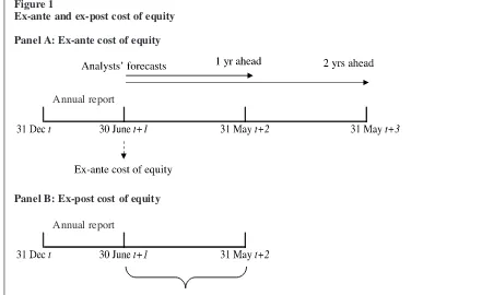
The ex-ante and ex-post measures of the cost of equity differ not only in the nature of the informa-tion on which they are based (analysts’ forecasts as opposed to realised returns), but also in the period of time when they are formed. The relationship be-tween the ex-ante and the ex-post measure of the cost of equity capital in terms of time is represent-ed in Figure 1.
As we can see, the ex-ante measure is based on analysts’ forecasts of earnings per share one and two years ahead at 30 June of year t+1, whereas the ex-post measure is based on realised returns (i.e. we estimate firm-specific asset-pricing mod-els running from June 1997 to May 2004). For the period June of year t+1 to May of year t+2, returns Figure 1
Ex-ante and ex-post cost of equity
Panel A: Ex-ante cost of equity
Panel B: Ex-post cost of equity
Annual report
Annual report
17Similar results obtain when using the three-factor model
proposed by Fama and French (1993).
18Material distortion refers to a mean favourable graph
dis-tortion index above 2.5%. The selection of this cut-off point is explained in detail in Section 3.2.2, when describing the meas-ure of graph distortion. The direction of the results remains unchanged if distorting and non-distorting portfolios include companies in the top and bottom 40% percentiles of the distri-bution of the variable used to measure graph distortion, re-spectively.
19Following prior literature on disclosure in Spain (e.g.
Espinosa and Trombetta, 2007), calculations start in June of year t+1, given that financial reporting regulation in Spain re-quires companies to release their annual report by that date at the latest.
to the graph distortion factor incorporated in the asset pricing models are calculated using the level of graph distortion in the annual report of year t. Then, when using the ex-ante measure of the cost of equity, the analysis of the effect of graph distor-tion is based on expectadistor-tions observed at a certain point time (June of year t+1). However, when em-ploying the ex-post measure, the analysis is based on monthly realised returns covering one year (from June of year t+1 to May of year t+2). Accordingly, the latter measure allows for two types of corrections: those arising from the aggre-gation of all investors’ decisions and those result-ing from the passresult-ing of time which permits new information to be impounded in stock prices.
3.2.2. Graph distortion measures Relative graph discrepancy (RGD) index
Graph distortion is measured in our study by using the relative graph discrepancy (RGD) index (Mather et al.,2005),20which is defined as
where g2 represents the actual height of the last column and g3is the proportionately correct height of the last column, based on the formula:
d1 = value of first data point (corresponding to the first column)
d2 = value of last data point (corresponding to the last column)
g1 = actual height of first column g2 = actual height of last column.
In the absence of distortion, the index takes the value of zero (0), that is, the change portrayed in the graph is the same as that observed in the data. The RGD takes a positive value both when an in-creasing trend is exaggerated and when a decreas-ing trend is understated. Negative values result from understatement of increasing trends and ex-aggeration of decreasing trends (Table 1, Panel A).
Measures of favourable and unfavourable graph distortion
The RGD index gives us an indication of the level of distortion of a particular graph, either if distor-tion is favourable or unfavourable to the firm. To test our hypotheses we need to isolate those distor-tions that are favourable to the company and design an indicator of favourable (unfavourable) graph distortion across all graphs in the annual report. Table 1
Measures of graph distortion
Panel A: Distortion measure for individual graphs
Trend in data Nature of distortion RGD
Increasing Exaggeration >0 Decreasing Understatement >0 Increasing Understatement <0 Decreasing Exaggeration <0
Panel B: Distortion measure across all graphs in the annual report
Graphs in the annual report RGDFAV RGDUNF
All graphs are properly constructed 0 0 There are favourably distorted graphs >0 >0 There are unfavourably distorted graphs
There are favourably distorted graphs >0 0 There is not any unfavourably distorted graph
There is not any favourably distorted graph 0 >0 There are unfavourably distorted graphs
20This measure was developed by Mather et al. (2005) to
overcome some of the limitations of the graph discrepancy index (GDI), the measure of graph distortion used in previous studies. The GDI is defined as 冠–a
b–1冡⫻100, where ais the
per-centage of change in centimetres depicted in the graph and bis the percentage of change in the data. We repeated all our analy-sis using the GDI, instead of the RGD, and results do not vary.
Favourably distorted graphs are those graphs manipulated to present a more favourable view of the company. Examples of favourable distortion are the magnification of a positive trend in sales growth or the understatement of a decreasing trend in the same variable. Conversely, understatement of an increasing trend in sales and exaggeration of a decreasing trend in this variable are examples of unfavourable distortion.
We measure the level of favourable distortion across all graphs included by a firm in the annual report as follows: when graph j is distorted to portray a more un-favourable view of the company.
n= total number of graphs in the annual report. The RGDFAV provides us with an indication of the mean level of favourable graph distortion in the annual report. This measure is increasing in the number of favourably distorted graphs and the cor-responding RGD indices. Zero (0) value for the RGDFAV indicates that the annual report does not contain any favourably distorted graph. Panel B in Table 1 describes the values that correspond to the RGDFAV measure depending on whether the an-nual report includes properly constructed, favourably, and unfavourably distorted graphs.
Similarly, we measure unfavourable graph dis-tortion across all graphs in the annual report as fol-lows: when graph j is distorted to portray a more favourable view of the company.
The RGDUNF is increasing in the number and the RGD of distorted graphs presenting a more un-favourable image of the company and takes the value of zero (0) when the annual report does not include any unfavourably distorted graph (Table 1, Panel B).
We also calculate mean favourable distortion index for financial (RGDFFAV) and non-financial graphs (RGDRFAV). These indices are defined in the same way as the RGDFAV but taking into con-sideration exclusively financial graphs (i.e. graphs depicting financial variables) for the RGDFFAV and non-financial graphs for the RGDRFAV.
In estimating the regression models we use the
fractional ranks of our graph distortion measures (RGDFAV, RGDUNF, RGDFFAV and RGDR-FAV). Fractional ranks for each of these measures are computed by dividing, within each year, the rank of a firm’s distortion measure by the number of firms in the sample in this year. The rank is in-creasing in the level of distortion.
Finally, in order to distinguish between material-ly and non-materialmaterial-ly distorted graphs we have to choose a cut-off point for the RGD measure. Mather et al. (2005) conclude that an RGD of 2.5% would be similar to a GDI of 5%, the cut-off point suggested by Tufte (1983) and used in previ-ous studies. This is why we decided to use the 2.5% cut-off point as suggested by Mather et al. (2005).22
3.2.3. Control variables
Following prior literature, we add a number of risk factors as controls in our regression models (i.e. number of analysts’ estimations, beta, lever-age, book-to-price ratio, volatility of profitability, growth, and disclosure). These factors are standard controls in the cost of equity literature, which widely documents their association with measures of the cost of equity (e.g. Gebhardt et al., 2001; Gietzmann and Ireland, 2005; Francis et al., 2008).
Number of estimates (NEST)
In order to proxy for the level of attention received by a company we use the number of analysts’ esti-mations of one-year-ahead EPS. This is a standard control variable used in disclosure-related studies. Starting from the seminal work by Botosan (1997), the previous literature has documented a strong in-fluence of the level of analysts’ attention on the re-lationship between disclosure and cost of equity capital.
Beta (BETA)
The capital asset pricing model (CAPM) predicts a positive association between the market beta of a stock and its cost of capital. However, previous studies do not consistently show such an expected relationship. While Botosan (1997) or Hail (2002) confirm the expected positive sign, Gebhardt et al. (2001) observe the expected sign but beta loses its significance when they add their industry measure. Finally, Francis et al. (2005) observe a negative re-lationship between beta and their measure of the cost of equity. We obtain the beta of each stock using a market model for the 60 months prior to
21As we are interested in obtaining an indicator of the level
of distortion, absolute values are used in order to avoid the off-setting of positive and negative values of the individual RGD’s.
22The direction of the results does not change when we use
a GDI of 10% as the cut-off point. This level of distortion was found to affect users’ perceptions in the study by Beattie and Jones (2002).
June of t+1, requiring, at least, 12 monthly return observations.
Leverage (LEV)
We measure leverage as the ratio between long-term debt and the market value of equity at 31 December of year t. Modigliani and Miller (1958) predict that the cost of equity should be in-creasing in the amount of debt in the financial structure of the company. This prediction is sup-ported by results of studies such as those by Gebhardt et al. (2001) or Botosan and Plumlee (2005). In line with previous literature we expect to find a positive relationship between leverage and the cost of equity capital.
Book-to-price ratio (BP)
This is the ratio between book value of equity and market value of equity at 31 December of year t. Prior research documents a positive association between the book-to-price ratio and average re-alised returns (e.g. Fama and French, 1993 and Davis et al., 2000) as well as different ex-ante measures of the cost of equity (e.g. Gebhardt et al., 2001 and Botosan and Plumlee, 2005). These re-sults are interpreted as evidence that the book-to-price ratio proxies for risk.
Volatility of profitability (V_NI)
Based on practitioners’ consideration of the vari-ability of earnings, Gebhardt et al. (2001) argue that this variable can be regarded as a source of risk. In our study, the volatility of the profitability of the firm is calculated as the standard deviation of net income scaled by mean of net income over a period of five years ending at December of year t.
Growth (GROWTH)
Following Francis et al. (2005) we control for the recent growth experienced by the company meas-ured as the log of 1 plus the percentage change in the book value of equity along year t.
Disclosure (RINDEX)
Finally, to test whether there is an interaction be-tween graph distortion and disclosure (H2), we in-troduce a measure of overall corporate disclosure. The relationship between corporate disclosure and the cost of equity is widely documented in the lit-erature (e.g. Botosan and Plumlee, 2002; Espinosa and Trombetta, 2007; Francis et al., 2008). As an indicator of the information provided by the company we use the disclosure index published annually by the business magazine Actualidad Económica. This index is based on the information disclosed by companies in their annual reports. These reports are reviewed by the panel of experts who assign a score to a list of information items. For each company, the scores for each item are then added up to obtain a global score intended to represent the disclosure policy of the entity. Finally, the disclosure index is calculated as the
ratio between the actual score of the company and the maximum possible score. Similar to Botosan and Plumlee (2002) or Nikolaev and Van Lent (2005), we use fractional ranks of the annual re-port indexes. Firms are ranked from 1 to N for each year and then the rank of each firm is divid-ed by the total number of firms in this year to ob-tain the fractional ranks.
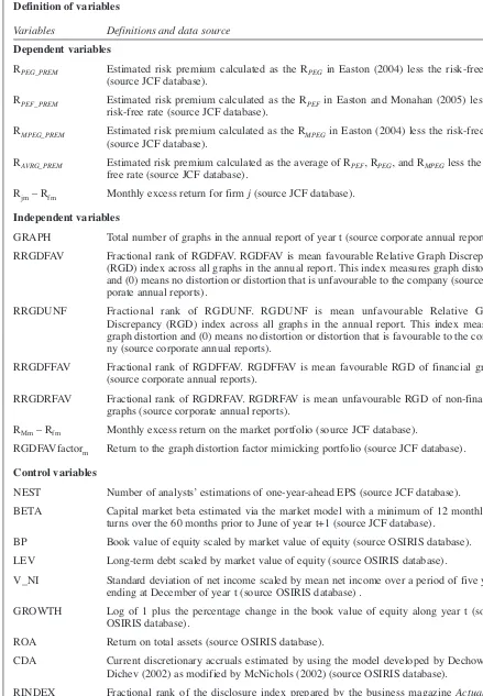
Table 2 provides a summary of the definition and data source of variables used in our analyses.
4. Results
4.1. Descriptive statistics
Descriptive statistics are presented in Table 3, where it can be seen that companies in our sample make wide use of graphs in their annual reports. At least one graph is included by 92% of the compa-nies and the mean number of graphs per annual re-port (GRAPH) is 16. These figures are similar to those observed for other countries (e.g. Beattie and Jones, 2001). Although not reported in Table 3, mean RGDFAV is higher than 2.5% for 38% of the companies included in our study; that is, more than one third of the companies in our sample have favourably distorted the graphs included in their annual reports above the cut-off point chosen as an indication of material distortion. Unfavourable distortions are less frequent; mean RGDUNF is higher than 2.5% for 11% of the companies in our sample.
The correlation matrix presented in Table 4 shows that our ex-ante measure of the cost of eq-uity is significantly correlated with all the risk proxies included in our study. As expected, the cost of equity is positively related to beta, book-to-price ratio, leverage and earnings variability and negatively related to growth and the number of es-timates that acts also as a proxy for corporate size. Table 4 also shows a significant negative correla-tion between the cost of equity and our indicators of graph distortion.
4.2. Multivariate analysis
4.2.1. Ex-ante measure of the cost of equity (RPEG_PREM)
This section presents the results obtained for the ex-ante measure of the cost of equity (i.e. the RPEG measure as developed by Easton, 2004). To asses the validity of this measure, we start our analysis by estimating a model similar to that de-veloped by Botosan and Plumlee (2005) and used to test the relation between the cost of capital and a number of indicators of firm risk. We estimate the following equation:
RPREMit+1= αi+ β1NESTit+ β2LEVit (1)
+ β3V_NIit+ β4BETAit+ β5BPit + β6GROWTHit+ eit,
Table 2
Definition of variables
Variables Definitions and data source
Dependent variables
RPEG_PREM Estimated risk premium calculated as the RPEG in Easton (2004) less the risk-free rate (source JCF database).
RPEF_PREM Estimated risk premium calculated as the RPEFin Easton and Monahan (2005) less the risk-free rate (source JCF database).
RMPEG_PREM Estimated risk premium calculated as the RMPEGin Easton (2004) less the risk-free rate (source JCF database).
RAVRG_PREM Estimated risk premium calculated as the average of RPEF, RPEG, and RMPEGless the risk-free rate (source JCF database).
Rjm– Rfm Monthly excess return for firm j(source JCF database).
Independent variables
GRAPH Total number of graphs in the annual report of year t (source corporate annual reports). RRGDFAV Fractional rank of RGDFAV. RGDFAV is mean favourable Relative Graph Discrepancy
(RGD) index across all graphs in the annual report. This index measures graph distortion and (0) means no distortion or distortion that is unfavourable to the company (source cor-porate annual reports).
RRGDUNF Fractional rank of RGDUNF. RGDUNF is mean unfavourable Relative Graph Discrepancy (RGD) index across all graphs in the annual report. This index measures graph distortion and (0) means no distortion or distortion that is favourable to the compa-ny (source corporate annual reports).
RRGDFFAV Fractional rank of RGDFFAV. RGDFFAV is mean favourable RGD of financial graphs (source corporate annual reports).
RRGDRFAV Fractional rank of RGDRFAV. RGDRFAV is mean unfavourable RGD of non-financial graphs (source corporate annual reports).
RMm– Rfm Monthly excess return on the market portfolio (source JCF database).
RGDFAVfactorm Return to the graph distortion factor mimicking portfolio (source JCF database).
Control variables
NEST Number of analysts’ estimations of one-year-ahead EPS (source JCF database).
BETA Capital market beta estimated via the market model with a minimum of 12 monthly re-turns over the 60 months prior to June of year t+1 (source JCF database).
BP Book value of equity scaled by market value of equity (source OSIRIS database). LEV Long-term debt scaled by market value of equity (source OSIRIS database).
V_NI Standard deviation of net income scaled by mean net income over a period of five years ending at December of year t (source OSIRIS database) .
GROWTH Log of 1 plus the percentage change in the book value of equity along year t (source OSIRIS database).
ROA Return on total assets (source OSIRIS database).
CDA Current discretionary accruals estimated by using the model developed by Dechow and Dichev (2002) as modified by McNichols (2002) (source OSIRIS database).
RINDEX Fractional rank of the disclosure index prepared by the business magazine Actualidad Económica for year t (source business magazine Actualidad Económica).
where:
RPREM= Proxy for the equity risk premium = RPEG – Rf
Rf= the risk-free rate, proxied by the interest rate on five-year Spanish Treasury bills.
The rest of the variables are defined in Table 2. We estimate all our models using the fixed ef-fects technique. The importance of using proper panel data estimation techniques when dealing with financial pooled data has been stressed by Nikolaev and Van Lent (2005) and Petersen (2005). If a simple OLS method is used to com-pute the estimated coefficients, their significance is very likely to be overstated. A traditional way to correct for this problem is to estimate yearly regressions and then take the average of the esti-mated coefficients, evaluating the statistical signif-icance of these estimates by using the Fama-Macbeth t-statistic. This corrects for cross-sectional dependence, but not for time depend-ence. Nikolaev and Van Lent (2005) show how important firm effects can be when studying cost of capital determinants for a pooled sample of companies. This is our reason for estimating our model by using the fixed effects technique.23
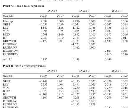
Results of estimating equation (1) are presented in Table 5, Panel B (Model 1). The coefficients of the number of estimates, leverage, and variability of profitability have the expected sign and are sta-tistically significant. The fact that the coefficients of beta and the book-to-price ratio are not statisti-cally significantly different from zero could be due to the use of the fixed effect estimation technique. Beta and the book-to-price are risk factors that are
specific for each company. Given that with the adopted estimation technique a specific intercept is estimated for each company, it is highly likely that the effect of these variables is already cap-tured by these constants. Overall, our results con-firm those already obtained for the Spanish market by Espinosa and Trombetta (2007) and support the validity of the measure of the cost of equity capi-tal and the choice of the control variables.
We now move on to the main part of our empir-ical study and insert in our specification the indi-cators of mean favourable and unfavourable graph distortion across all graphs included in the annual report. Specifically, we now estimate the following equation (Model 2):
RPREM it+1= αi+ β1NESTit+ β2LEVit (2)
+ β3V_NIit+ β4BETAit+ β5BPit
+ β6GROWTHit+ β7RRGDFAVit + β8RRGDUNFit+ εit
All variables are defined in Table 2.
We now find that favourable graph distortion is significantly and negatively related to the ex-ante measure of the cost of equity. A negative coeffi-cient is also observed for unfavourable graph dis-tortion but results show that it is insignificantly different from zero. These results suggest that favourably distorted graphs introduce a bias on users’ perceptions. According to our results, annu-al report users perceive a better image of corporate performance when the annual report includes Table 3
Descriptive statistics
Mean Std. Dev. Minimum Maximum 25th perc. 50th perc. 75th perc.
RPEG_PREM 5.972 4.448 –0.693 25.031 3.134 5.128 7.682
NEST 15.927 9.103 1 40 9 16 21 BETA 1.125 0.549 0.034 4.594 0.773 1.038 1.348 BP 0.637 0.403 0.049 3.018 0.362 0.558 0.818 LEV 0.398 0.603 0 6.315 0.065 0.221 0.469 V_NI 0.579 1.646 –2.670 19.930 0.180 0.320 0.558 GROWTH 0.103 0.235 –1.769 1.515 0.013 0.079 0.148 GRAPH 16.087 15.461 0 84 4.25 12 23 RGDFAV 0.106 0.307 0 3.685 0 0 0.095 RGDUNF 0.012 0.062 0 0.878 0 0 0 RGDFFAV 0.108 0.326 0 3.685 0 0 0.068 RGDRFAV 0.043 0.151 0 1.5 0 0 0 ROA 6.273 5.820 –21.190 28.100 2.680 5.145 8.150 CDA 0.021 0.065 –0.318 0.238 –0.011 0.017 0.048 INDEX 0.637 0.150 0.230 0.960 0.550 0.630 0.750 The sample consists of 259 firm-year observations for the period 1996–2002. The definition of variables is pro-vided in Table 2.
23However, at least for our main analysis, we also provide
the results obtained by running an OLS regression on the pooled sample. These results can be found in Table 4, Panel A.
94
A
CCO
U
N
T
IN
G
A
N
D
BU
S
IN
E
S
S
RE
S
E
A
RCH
Table 4
Correlation matrix
RPEG_PREM NEST BETA BP LEV V_NI GROWTH RGDFAV RGDUNF RGDFFAV RGDRFAV ROA CDA
NEST –0.200
(0.001)
BETA 0.222 –0.124
(0.000) (0.046)
BP 0.379 –0.329 0.099
(0.000) (0.000) (0.112)
LEV 0.172 0.161 0.023 0.417
(0.006) (0.009) (0.707) (0.000)
V_NI 0.192 –0.121 0.168 0.091 –0.020
(0.002) (0.053) (0.007) (0.144) (0.745)
GROWTH –0.165 0.104 –0.011 –0.193 –0.028 0.088
(0.008) (0.093) (0.854) (0.002) (0.651) (0.159)
RGDFAV –0.175 0.172 0.031 –0.036 0.081 –0.096 0.014
(0.005) (0.005) (0.616) (0.559) (0.195) (0.122) (0.822)
RGDUNF –0.077 0.180 –0.014 –0.073 0.095 –0.041 0.066 0.339
(0.217) (0.004) (0.825) (0.243) (0.127) (0.516) (0.291) (0.000)
RGDFFAV –0.202 0.112 0.025 –0.048 0.034 –0.086 0.089 0.872 0.276
(0.001) (0.073) (0.689) (0.444) (0.590) (0.168) (0.152) (0.000) (0.000)
RGDRFAV –0.102 0.268 –0.004 –0.024 0.131 –0.057 –0.101 0.597 0.311 0.301
(0.103) (0.000) (0.955) (0.698) (0.036) (0.357) (0.106) (0.000) (0.000) (0.000)
ROA –0.250 0.065 –0.153 –0.343 –0.543 –0.012 0.213 –0.046 –0.111 –0.010 –0.054
(0.000) (0.298) (0.014) (0.000) (0.000) (0.853) (0.001) (0.456) (0.073) (0.871) (0.387)
CDA 0.093 –0.088 0.007 0.062 0.076 –0.081 0.002 0.131 –0.021 0.090 0.071 0.166
(0.163) (0.191) (0.920) (0.356) (0.259) (0.225) (0.976) (0.050) (0.754) (0.177) (0.288) (0.013)
RINDEX –0.220 0.466 –0.003 –0.064 0.247 –0.055 0.010 0.212 0.238 0.170 0.283 –0.323 –0.143
(0.000) (0.000) (0.959) (0.304) (0.000) (0.375) (0.876) (0.001) (0.000) (0.006) (0.000) (0.000) (0.032)
Table reports Spearman correlations. Significance levels are shown in brackets. The definition of variables is provided in Table 2.
graphs that have been distorted to portray a more favourable view of the company. The same is true if we focus our attention only on financial graphs (RRGDFFAV), as we do in Model 3. These results support our hypothesis H1. The information repre-sented in graphs is usually included in the financial statements or other parts of the annual report. However, users get a different picture of the com-pany when the annual report includes favourably distorted graphs. These results are consistent with the experimental evidence of the impact of im-properly constructed graphs on subjects’ choices
provided by Arunachalam et al. (2002). They ob-serve that students’ decisions are affected by graph design. We extend these results by showing that, in a real setting, experts’ (analysts’) forecasts are biased because of distorted graphs included in annual reports.
We test the robustness of these results to the choice of the ex-ante measure of the cost of equity and to the inclusion of additional control variables. As for the proxy for the cost of equity, we calcu-late two alternative measures: RPEFand RMPEG. The definition of these measures is given in the appen-Table 5
Regression of the ex-ante measure of cost of equity (RPEG_PREM) on risk proxies and graph distortion
Model 1: RPEG_PREM it+1= αi+ β1NESTit+ β2LEVit+ β3V_NIit+ β4BETAit+ β5BPit+ β6GROWTHit+ εit
Model 2: RPEG_PREM it+1= αi+ β1NESTit+ β2LEVit+ β3V_NIit+ β4BETAit+ β5BPit+ β6GROWTHit + β7RRGDFAVit+ β8RRGDUNFit+ εit
Model 3: RPEG_PREM it+1= αi+ β1NESTit+ β2LEVit+ β3V_NIit+ β4BETAit+ β5BPit+ β6GROWTHit
+ β9RRGDFFAVit+ β10RRGDRFAVit+ εit
Panel A: Pooled OLS regression
Model 1 Model 2 Model 3
Variable Coeff. P-val Coeff. P-val Coeff. P-val
Intercept 4.382 0.000 4.936 0.000 5.101 0.000 NEST –0.059 0.039 –0.051 0.091 –0.057 0.064 LEV 1.149 0.128 1.122 0.145 1.136 0.143 V_NI 0.096 0.325 0.075 0.435 0.083 0.403 BETA 0.791 0.149 0.892 0.105 0.895 0.096 BP 2.089 0.010 2.111 0.010 2.053 0.011 GROWTH –2.172 0.087 –2.131 0.097 –1.839 0.160 RRGDFAV –1.721 0.072
RRGDUNF 0.162 0.900
RRGDFFAV –2.604 0.005
RRGDRFAV 0.910 0.530
Adj. R2 0.135 0.138 0.149 Panel B. Fixed effects regressions
Model 1 Model 2 Model 3
Variable Coeff. P-val Coeff. P-val Coeff. P-val
NEST –0.147 0.011 –0.130 0.027 –0.126 0.032 LEV 2.537 0.004 2.491 0.005 2.516 0.005 V_NI 0.264 0.022 0.270 0.021 0.279 0.018 BETA –0.378 0.453 –0.271 0.593 –0.293 0.567 BP –0.109 0.912 –0.127 0.897 –0.182 0.851 GROWTH 0.160 0.867 0.208 0.831 0.296 0.766 RRGDFAV –2.351 0.013
RRGDUNF –0.182 0.828
RRGDFFAV –2.230 0.015
RRGDRFAV –1.032 0.260
Adj. R2 0.547 0.554 0.555
The sample consists of 259 firm-year observations for the period 1996–2002. The definition of variables is pro-vided in Table 2. Estimates of the firm-specific constant terms are omitted for readability.
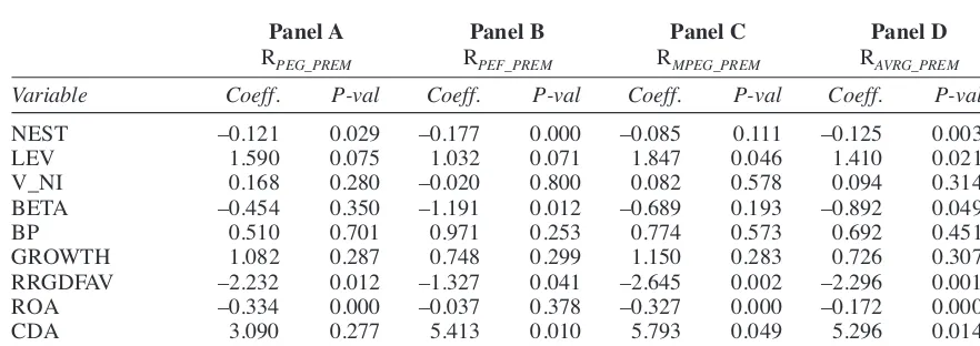
dix. We also use the average (RAVRG) of the three proxies calculated in our study. Additionally, we check if our results are driven by factors such as corporate performance or accruals quality. Prior literature documents a positive association be-tween corporate performance and graph distortion (e.g. Beattie and Jones, 1999, 2000). Therefore, the effect of graph distortion on the cost of equity that we observe in this study could be driven by the fact that distorting companies are also those with the highest performance. Hence, we add a measure of corporate performance (i.e. ROA) as a control variable. Second, Francis et al. (2005) and Francis et al. (2008) show the existence of a posi-tive relationship between the cost of equity capital and the (poor) quality of accruals. The negative re-lationship between graph distortion and the cost of equity observed in this study could be reflecting this association. Therefore, we test for the robust-ness of our results by adding a measure of accruals quality (i.e. discretionary accruals) to our model (CDA).24
Table 6 reports the results of these sensitivity analyses and shows that the effect of favourable graph distortion on the ex-ante cost of equity is ro-bust to the choice of the measure of the cost of eq-uity. Favourable graph distortion is found to be negatively and significantly related to all the alter-native measures of the ex-ante cost of equity cal-culated in our study. Additionally, we observe that, although corporate performance and accruals qual-ity can be highly significant variables in explain-ing the ex-ante cost of equity, its inclusion in the model does not qualitatively change our results.
That is, the effect of favourable graph distortion on the ex-ante measures of the cost of equity remains.
Interaction analysis
To investigate whether the relationship between graph distortion and the ex-ante measure of the cost of equity varies depending on the overall level of disclosure, as stated in our second hypothesis, we introduce a measure of the voluntary informa-tion provided by the company in their annual re-port (RINDEX) and an interaction term between disclosure and graph distortion. Specifically, we estimate the following equation:
RPREMit+1= αi+ β1NESTit+ β2LEVit (3)
+ β3V_NIit+ β4BETAit+ β5BPit+ β6GROWTHit + β7RRGDFAVit+ β8RINDEXit
+ β9RRGDFAVit* RINDEXit+ εit All variables are defined in Table 2.
Table 7, Panel A presents the results of the esti-mation of Equation (3). Consistent with the results reported previously, the coefficient on RRGDFAV is found to be negative and significant. A negative relationship is also observed between the overall level of disclosure and the cost of equity, although it is not significant at conventional levels. Finally, the interaction term is positive and significant, which means that graph distortion and disclosure interact in shaping their effects on the cost of equi-ty. Since the sign of the interaction term is posi-Table 6
Regression of the cost of equity on risk proxies and graph distortion using fixed effects
RPREM it+1= αi + β1NESTit+ β2LEVit+ β3V_NIit+ β4BETAit+ β5BPit+ β6GROWTHit+ β7RRGDFAVit
+ β9ROAit+ β10CDAit+ εit
Panel A Panel B Panel C Panel D
RPEG_PREM RPEF_PREM RMPEG_PREM RAVRG_PREM
Variable Coeff. P-val Coeff. P-val Coeff. P-val Coeff. P-val
NEST –0.121 0.029 –0.177 0.000 –0.085 0.111 –0.125 0.003 LEV 1.590 0.075 1.032 0.071 1.847 0.046 1.410 0.021 V_NI 0.168 0.280 –0.020 0.800 0.082 0.578 0.094 0.314 BETA –0.454 0.350 –1.191 0.012 –0.689 0.193 –0.892 0.049 BP 0.510 0.701 0.971 0.253 0.774 0.573 0.692 0.451 GROWTH 1.082 0.287 0.748 0.299 1.150 0.283 0.726 0.307 RRGDFAV –2.232 0.012 –1.327 0.041 –2.645 0.002 –2.296 0.001 ROA –0.334 0.000 –0.037 0.378 –0.327 0.000 –0.172 0.000 CDA 3.090 0.277 5.413 0.010 5.793 0.049 5.296 0.014 Adj. R2 0.630 0.599 0.653 0.659
The sample consists of 259 firm-year observations for the period 1996–2002. The definition of variables is pro-vided in Table 2. Estimates of the firm-specific constant terms are omitted for readability.
24To obtain this measure we use the model developed by
Dechow and Dichev (2002) as modified by McNichols (2002).
tive, results indicate that the effect of graph distor-tion on the cost of equity is moderated by the level of overall disclosure. Stated in other words, the ef-fect of graph distortion on the cost of equity is par-tially (or eventually completely) offset by its interaction with the overall level of disclosure. To get a clearer picture of the interaction between graph distortion and disclosure we dichotomise the RINDEX variable and estimate the following equation:
RPREM it+1= αi+ β1NESTit+ β2LEVit (4)
+ β3V_NIit+ β4BETAit+ β5BPit+ β6GROWTHit + β7RRGDFAVit+ β8RINDEX_Dit
+ β9RRGDFAVit* RINDEX_Dit+ εit
where all the variables are defined as before except for:
RINDEX_D = A dichotomy variable which, in Panel B (C), takes the value of one (1) when the value of the RINDEX is in the top 50% (33%) per-centile of the distribution of this variable, and a value of zero (0) otherwise.
Results of this estimation are presented in Table 7, Panels B and C. Since the selection of the cut-off point used to dichotomise the RINDEX vari-able is arbitrary, Tvari-able 7 reports the results obtained by using two different cut-off points. In panel B, the set of high disclosers comprises those
companies the disclosure index of which is above the median, while in Panel C high disclosers are those firms falling in the top 33% percentile of the distribution of the RINDEX variable.
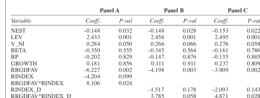
Consistent with the results presented in Panel A, we find that the cost of equity is negatively associ-ated with RRGDFAV and positively relassoci-ated to the interaction term. The dichotomisation of the vari-able RINDEX facilitates the interpretation of the results. When RINDEX_D takes the value of zero (0), the relationship between graph distortion and the cost of equity is given by β7 and is negative, both in Panels B and C. This means that for low disclosers, graph distortion is negatively related to the cost of equity. However, when RINDEX_D takes the value of one (1), the effect of graph dis-tortion is given by the addition of the coefficients on RRGDFAV and the interaction term (i.e. β7 + β9). This addition results in a negative figure (–0.413) in Panel B, which is much lower than the coefficient on RRGDFAV, and a positive figure (0.962) in Panel C. Thus, for transparent compa-nies, disclosure partially removes the effect of graph distortion (Panel B) or even transforms it into a positive effect (Panel C). These results indi-cate that disclosure moderates the relationship be-tween graph distortion and the cost of equity and provide support for our second hypothesis. Furthermore, differences between Panels B and C indicate that the moderating effect is increasing in Table 7
Regression of the cost of equity on risk proxies, graph distortion, and disclosure using fixed effects
Model 1: RPEG_PREM it+1(Panel A) = αi + β1NESTit+ β2LEVit+ β3V_NIit+ β4BETAit+ β5BPit+ β6GROWTHit
+ β7RRGDFAVit+ β8RINDEXit+ β9RRGDFAVit* RINDEXit+ εit
Model 2: RPEG_PREM it+1(Panels B–C) = αi + β1NESTit+ β2LEVit+ β3V_NIit+ β4BETAit+ β5BPit+ β6GROWTHit
+ β7RRGDFAVit+ β8RINDEX_Dit+ β9RRGDFAVit* RINDEX_Dit+ εit
Panel A Panel B Panel C
Variable Coeff. P-val Coeff. P-val Coeff. P-val
NEST –0.148 0.032 –0.148 0.028 –0.153 0.022 LEV 2.433 0.001 2.456 0.001 2.495 0.001 V_NI 0.284 0.050 0.266 0.066 0.276 0.058 BETA –0.350 0.555 –0.345 0.564 –0.161 0.786 BP –0.202 0.829 –0.147 0.876 –0.135 0.885 GROWTH 0.181 0.856 0.111 0.911 0.237 0.809 RRGDFAV –6.227 0.002 –4.198 0.003 –3.909 0.002 RINDEX –4.204 0.099
RRGDFAV*RINDEX 8.106 0.024
RINDEX_D –1.517 0.178 –2.093 0.143 RRGDFAV*RINDEX_D 3.785 0.058 4.871 0.028 Adj. R2 0.564 0.561 0.565
The sample consists of 259 firm-year observations for the period 1996–2002. The definition of variables is pro-vided in Table 2. Estimates of the firm-specific constant terms are omitted for readability.
the level of disclosure, so that when transparency is sufficiently high, the relationship between graph distortion and the ex-ante measure of the cost of equity becomes positive. Results suggest that while at low levels of transparency graph distor-tion remains undetected, high levels of disclosure uncover graph distortion, which results in an in-crease in the risk perceived by users. Hence, users’ predictions can only be potentially affected by graph distortion when the level of information pro-vided by the company is low.
So far we have used an ex-ante measure of the cost of equity based on analysts’ estimations of earnings per share. Hence, our results could be in-terpreted as evidence that graph distortion affects users’ (analysts’) perceptions of corporate per-formance. However, it is important to check that the market is able to correct individuals’ biases. With this aim, in the next section we present the results obtained using average ex-post returns as a proxy for the cost of equity.
4.2.2. Ex-post measure of the cost of equity (stock returns)
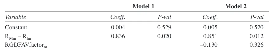
As a starting point in our ex-post analysis, we es-timate a one-factor asset-pricing model for each of the 68 companies in our sample.25The average co-efficients and adjusted R’s squared of these esti-mations are presented in Table 8 (Model 1).
Results show a mean beta of 0.84 and a mean ad-justed R-squared of 26.4%. We proceed by adding a factor aimed at representing favourable graph distortion (RGDFAVfactor). Specifically, we esti-mate the following equation:
Rjm – Rfm= aj+ bj(RMm– Rfm) (5)
+ cjRGDFAVfactorm+ εjm
where:
Rjm– Rfm= monthly excess return for firm j. RMm– Rfm= monthly excess return on the market portfolio
RGDFAVfactorm = return to the graph distortion factor mimicking portfolio
Average coefficients obtained from firm-specific estimations of Equation (5) are reported in Table 8 (Model 2). Results show that stock returns are not affected by the distortion of graphs includ-ed in the annual report. The coefficient of the RGDFAV factor is negative but it is insignificant-ly different from zero. Hence, we find support for our hypothesis H3. Results (unreported) are simi-lar when we construct the RGDFAV factor relay-ing on favourably distorted graphs representrelay-ing financial variables. Although these variables might exert a higher influence on users’ decisions than non-financial variables, results show that stock re-turns are not affected by the distortion of financial graphs. These results are in accordance with the EMH and suggest that decision makers (at the ag-gregated level) are able to see through distortion. Their decisions cannot be biased by means of ‘rosy’ graphs depicting a much more favourable view of corporate performance than that reflected in the fi-nancial statements. Nonetheless, results presented in the previous section show the existence of a negative and significant relationship between favourable graph distortion and the ex-ante meas-ure of the cost of equity. One way to explain these apparently contradicting findings is that individu-als’ perceptions can be biased because of distorted graphs, but the aggregation process performed by the stock market leads to unbiased decisions. Prior research shows that the aggregation of individual’s predictions leads to higher levels of accuracy (e.g. Solomon, 1982 and Chalos, 1985). Furthermore, Table 8
Firm-specific regressions of stock returns on the market portfolio and the graph distortion factor
Model 1: Rjm– Rfm= aj+ bj(RMm– Rfm) + εjm
Model 2: Rjm– Rfm= aj+ bj(RMm– Rfm) + cjRGDFAVfactorm+ εjm
Model 1 Model 2
Variable Coeff. P-val Coeff. P-val
Constant 0.004 0.529 0.005 0.520 RMm– Rfm 0.836 0.020 0.851 0.012 RGDFAVfactorm –0.130 0.326
R-squared 0.264 0.296
The table reports the average coefficient estimates obtained from the estimation of the asset-pricing models for each company included in our sample. A minimum of 18 monthly stock returns for the period June 1997 to May 2004 is required. The definition of variables is provided in Table 2.
25A minimum of 18 monthly returns is required in these
es-timations.