A new method to estimate the level and
distribution of household human capital with
application
Camilo Dagum
a,*, Daniel J. Slottje
b aDepartment of Statistics,Uni6ersity of Bologna,6ia Belle Arti 41,40126 Bologna, Italy bDepartment of Economics,Southern Methodist Uni
6ersity,Dallas,TX75275-0496, USA
Abstract
This study introduces a new approach that enables, for the first time, the estimation of national and personal human capital (HC) in money value. National HC is estimated on the basis of the life cycle mean earned income by age using sample survey data which are smoothed with local linear filters. Personal HC is treated as a dimensionless latent endoge-nous variable. The estimation of each economic unit HC as a latent variable is benchmarked by the estimation of the average national HC in order to obtain estimates in money value. A model is fitted to study the distribution of personal HC. This new approach is illustrated using data from the U.S. Federal Reserve Board sample survey on income and wealth distributions. The new theoretical developments and empirical results provide the framework to advance socioeconomic policies on issues of endogenous economic growth with economic efficiency and social equity, hence, to deal with the problems of poverty and socially unacceptable inequality. This study is integrated with a discussion and evaluation of alternative methods of HC estimation proposed in the literature, i.e. the prospective, retrospective, and educational stock. It includes a brief comment on the contributions of the Chicago School which specifies an earning income function within the HC conceptual framework, without dealing with HC estimation. © 2000 Elsevier Science B.V. All rights reserved.
JEL classification:J24; J41
Keywords:Prospective method; Retrospective method; Educational stock; Earned income function; Size distribution of human capital
* Corresponding author.
E-mail addresses:[email protected] (C. Dagum)., [email protected] (D.J. Slottje). 0954-349X/00/$ - see front matter © 2000 Elsevier Science B.V. All rights reserved.
1. Introduction
The concept of functional income distribution was introduced by Ricardo (1817). The first research on the personal (size) distribution of income was done by Pareto (1895, 1896, 1897). He was the first to specify, estimate and analyze a model of income distribution. Both the functional and personal income distributions are assumed to be generated by two variable factors, human capital (that generates earned income); and capital (that generates other incomes). The theoretical produc-tion funcproduc-tion that underlies both of these concepts of distribuproduc-tion includes labor as an argument. Unfortunately, labor is generally measured in these production functions as man-hours worked or as persons employed full-time per year. While it is useful to partition the labor force (into full-time, part-time and unemployed workers) for labor market studies, it can be misleading to do so when analyzing economic processes involving production, growth, distribution and social welfare. The usual specification of the production function is,
Q=F(L,K) (1a)
In virtually all micro and macro applications of the production function, what is really of interest is of course, employed human capital (H) and capital (K), not just a generic labor stockL. Output is produced, income is earned and input prices are set based on the quality of the experience, training and schooling embodied in labor (its skill set), not just based on the magnitude of the labor stockL. Denison (1967, 1974) was among the first to make this adjustment in empirical specifications of the production function and Dagum (1978) was among the first to note this in work on the functional income distribution. Thus, the production function should be specified as,
Q=F(H,K) (1b)
The purpose of our study is to quantify human capitalHand to examine its size distribution empirically. By doing so, a better understanding of the relationship between the functional income distribution and the personal income distribution can be achieved. The theoretical and applied relevance of an integration of these sub-fields becomes obvious when it is observed that the functional income distribu-tion deals with the factor price formadistribu-tion and the allocadistribu-tion of total income among the factors of production. Whereas, the personal income distribution deals with the allocation of total income among the set of families, households or their disaggrega-tion by various retained attributes.
y=8(h,k), 8h\0, 8k\0, (h,k)\0, (2)
wherey stands for personal income,hfor the stock of HC, andk for the stock of wealth (non-human capital), corresponding to the economic units which are the object of inquiry.
The IGF plays a fundamental role in the analysis and linking of the functional and personal income distribution, the integration of the micro and the macroeco-nomic processes concerning the generation and distribution of income, and in providing the basic analytical knowledge for the design of policies regarding growth and development. For further consideration on the IGF and its role to deal with the linking of the functional and personal income distribution, see Dagum (1994, 1999). This fundamental topic will not be discussed in this study because it falls outside the purpose of this research.
The processes considered above give a special role to investment in HC and in a socioeconomic infrastructure aimed at a more equitable income and wealth distri-bution, with less poverty and with the elimination of social exclusion. For these reasons, and sinceh is a latent variable, we have to have information aboutkand a selected set of indicators to arrive at a robust estimation of the personal or size distribution ofh. The most important sources of information towards this end are the sample surveys of income and wealth distribution data.
2. Human capital: a brief historical review
The concept of human capital was first introduced and estimated by Petty (1690). Cantillon (1755) discussed the concept of HC and estimated the cost of rearing a child until working age. Smith (1776) presented a clear analysis of the concept of HC and included it as a part of the ‘general stock (human and non-human capital) of any country or society’, where this general stock is composed of the following resources, (i) of all useful machines and instruments of trade which facilitate and abridge labor; (ii) of all those profitable buildings which are the means of procuring a revenue; (iii) of the improvements of land; and (iv) of the acquired and useful abilities of all the inhabitants or members of the society. Afterwards, he added, the ‘‘acquisition of such talents, by the maintenance of the acquirer during his education, study, or apprenticeship, always cost a real expense, which is acapital
fixed and realized, as it were, in his person’’.
Although Smith did not engage himself either in any human capital estimation or in the proposition of a particular approach to estimate it, he implicitly adopted the cost of production approach. He advanced the following five basic determinants of inequalities of earned income (Smith, 1776), ‘‘first, the agreeableness or disagree-ableness of the employment themselves; secondly, the easiness and cheapness, or the difficulty and expense of learning them; thirdly, the constancy or inconstancy of employment in them; fourthly, the small or great trust which must be reposed in those who exercise them; and, fifthly, the probability or improbability of success in them’’.
Since Smith until the middle of the 20th century, distinguished economists, statisticians and econometricians accepted the concept of HC as a proxy for genetic and acquired skills and abilities. Among them, we mention Bentham, Say, Senior, J.S. Mill, List, von Thunen, Engel, Walras, Marshall, I. Fisher, Pareto, Beneluce, Nicholson, de Foville, Barriol, Dublin, Lotka, Gini, Mortara, Pietra, J.M. Clark, Ros Jimeno and Sensini. With the exception of Bentham, Say, Senior, Mill, List, Walras and von Thunen, all the others dealt with some form of quantitative HC estimation. On the other hand, based on ethical considerations, Mill and Marshall objected the notion of HC. Similar position is taken by Perroux (1974), who used instead the concept of human resources.
More generally, as Willis (1986) observed, ‘‘the term ‘earnings function’ has come to mean any regression of individual wage rates or earnings on a vector of personal, market, and environmental variables thought to influence the wage’’.
Departing from the approach of Gibrat (1931), Rutherford (1955), Mandelbrot (1960, 1963), who considered chance as a dominant variable determining the levels of earnings, whereas individual choice was not, Mincer (1958, 1970) specified the first model of earned income derived from individual investment behavior, i.e. individual choice. He took ‘‘the length of training as the basic source of heterogene-ity of labor incomes’’ (Mincer, 1970). This training raises productivheterogene-ity and post-pones the entrance age into the labor market. The specification of Mincer’s earning function is derived from four highly simplifying assumptions, where the first and the fourth are only mathematical devices to rationalize an obvious explanatory variable, i.e. years of schooling, which suggests instead a direct specification based on factual observations.
The assumptions of Mincer (1970) are,
A.1: ‘‘In a competitive equilibrium, the distribution of earnings is such that the present values of future earnings discounted at the market rate of interest are equalized al the time training begins’’.
A.2: ‘‘The model is formulated in terms of training periods which are completed before earnings begin’’.
A.3: ‘‘No further investments in human capital are undertaken by individuals after completion of their schooling’’.
A.4: ‘‘The flow of their earnings is constant throughout their working lives’’. Becker (1975) extended Mincer’s approach by including postschool investments in HC, which can be disaggregated to deal with different types of investment, such as, training, health, and migration. After a sequence of simplified assumptions, Becker specified earned income as a function of years of schooling and postschool investments in HC, i.e.
logEt=logE0+rs+rPt, (3) where, in periodt, E stands for earnings, s for years of schooling, andP for net postschool investment, whereas E0 stands for raw earnings, i.e. earnings without schooling and postschool investment in HC; r, r and E0 are parameters to be estimated.
3. Human capital: methods of estimation
3.1.The prospecti6e approach
This was the first method used to estimate personal and national HC. Petty (1690) was the most prominent founder of the Political Arithmetic school of economics and a precursor to modern applied econometrics. He was the first author to apply the prospective method to estimate the HC of a nation with the purpose of assessing the loss sustained by a plague, by the slaughter of men in war, and by migration. His method purported to offer also a sound base for taxation and to evaluate the power of a nation.
Petty estimated the HC of England as the difference between his estimation of national income (£42 million) and property income (rent of land 8 millions and profit 8 millions) capitalized in perpetuity at a 5% interest rate, arriving at a total HC estimation of £520 million; or a per capita estimation of £80. Although Petty’s approach was a very crude one, it had the merit of raising the issue, giving an answer, and making an economic and social interpretation of the result obtained. A rigorous scientific approach, that applies actuarial mathematics to estimate individual human capital, was developed by Farr (1853). He provided the basic approach and the scientific standard to estimate the gross and the net economic value of a human being to offer it as a basis for an equitable taxation of individual physical and human capital stocks. Farr (1853) stated that ‘‘the characteristic of life property in wages, …, is that it is inherent in man, and is the value of his services — of the direct product of his skill and industry, …, [which] is not the less on that account property’’.
Observing the salary and the maintenance cost of agricultural laborers by age, and adopting a 5% discount rate and a life table, Farr estimated £349 to be the average gross value of an agricultural laborer, £199 to be the average maintenance cost, hence, he estimated £150 to be the average net HC value.
Wittstein (1867) applied Farr’s prospective method to estimate the HC of an individual at several ages. His results are distorted by the adoption of the unaccept-able postulate that at birth, the flow of incomes of an individual throughout his life and the expenses of a given individual’s maintenance are equal. This assumption contradicts human history which testimonies that, in average, individuals add to the national well-being of societies.
Marshall (1922) adopted Wittstein’s controversial postulate and stated that, ‘‘many writers assume, implicitly at least, that the net production of an average individual and the consumption during the whole of his life are equal, or in other words, that he would neither add to nor take from the national well-being of a country, …. On this assumption, the above two plans of estimating his value would be convertible; and then, of course, we should make our calculations by the latter and easier (the consumption) method’’.
A French actuarian, Barriol (1910) used the prospective method to estimate the social value of an individual. By social value, he meant the amount that an individual restores to society out of his earnings. Barriol’s social value would be equivalent to Farr’s present net value of an individual at birth.
de Foville (1905) estimated HC in France by capitalizing labor income net of consumption expenditures. Fisher (1927) applied Farr’s prospective method to estimate average U.S. human capital and then, by applying a mortality table, he advanced an estimation of the cost of preventable illness.
Following Farr’s seminal contribution, Dublin and Lotka (1930) published an influential research monograph on the money value of a human being. Their model is now discussed.
LetV(x) be the net value of a person of agex;6x=(1+i)−xthe present value
of a unit of money duexyears later, whereiis the discount rate;p(a,x)=l(a+x)/
l(x) the probability at age a of living to age a+x; l(x) the population of age x;
y(x) the annual earnings of a person of agex;E(x) the annual rate of employment at agex, hence,U(x)=1−E(x) is the annual rate of unemployment at agex; and
c(x) is the annual cost of living of a person at age x. For the sake of notational simplification, we work with age x, instead of x+1/2 as the representative age in a calendar year.
The net value of a human being (net HC) at agea is the present actuarial value of a flow of net annual expected earnings, i.e.
V(a)= %
x=a
6x−a[y(x)E(x)−c(x)]p(a,x) (4)
Hence, at birth,
V(0)= %
x=0
6x[y(x)E(x)−c(x)]p(0,x), (5)
i.e. Barriol’s social value of an individual.
It follows from Eq. (4) that the net cost at agea of rearing a person from birth to agea is,
C(a)= % a−1
x=0
(1+i)a−x[c(x)−y(x)E(x)]
p(x,a) (6)
The denominator in Eq. (6) means thatC(a) includes the per capita net cost for the surviving population at agea of those that died at age xBa.
It follows from Eqs. (4) – (6) that,
V(a)=(1+i) a
p(0,a)
!
%
x=a
6x[y(x)E(x)−c(x)]p(0,x)
"
=V(0)(1+i)a
p(0,a)+C(a).
Hence,
C(a)=V(a)−V(0)(1+i) a
The gross HC at agea is obtained from Eq. (4) after making c(x)=0 for allx, i.e.
Gross HC(a)= %
x=a
6x−ay(x)E(x)p(a,x) (8)
In the second half of the 20th century, little research was done using the prospective method. Among them, we mention the comprehensive estimates of Jorgenson and Fraumeni (1989). These authors proposed a new system of national accounts for the U.S. economy that included market and non-market economic activities with the purpose of assessing the role of capital formation in U.S. economic growth. Jorgenson and Fraumeni (1989) defined full labor compensation as the sum of market and non-market labor compensation after taxes. They assumed (p. 233) that expected incomes in future time periods are equal to the incomes of individuals of the same sex and education, but with the age that the individual will have in the future time period, adjusted for increases in real income. The authors estimated the human and non-human capital for the US from 1949 to 1984. They used hourly labor compensation annually for individuals classified by the two sexes, 61 age groups, and 18 education groups for a total of 2196 groups. Macklem (1997) estimated quarterly per capita HC for Canada, from 1963 to the second quarter of 1994. He computed aggregate HC as the expected present value of aggregate labor income net of government expenditures based on an estimated bivariate vector autoregressive (VAR) model for the real interest rate and the growth rate of labor income net of government expenditures.
3.2.The retrospecti6e approach
Although A. Smith implicitly proposed the cost of production (‘‘a man educated at the expense of much labor and time’’) as a main determinant of differential wages, Engel (1883) was the first to advance and apply the retrospective method of HC estimation. He was not attracted to the prospective method because of the weight he gave to outstanding outliers such as Goethe, Newton, and Benjamin Franklin. He argued that the HC of these extreme cases could not be estimated for lack of knowledge about their future earnings, instead, he said it was possible to estimate their rearing costs to their parents.
Studying the budget of Prussian working families, Engel adopted very crude assumptions to arrive at the estimation of the cost of production. He considered three (lower, middle, and upper) classes, assumed a costci(i=1, 2, 3) at birth of theith class, increasing it annually in an arithmetic progression until the age of 25. At 26, he considered that a human being was fully produced. For each year of age, Engel increased the costciat birth by the constant amountciqi, hence, the annual cost of rearing a person of agexB26, belonging to theith class, becomesci+xciqi. Adding the historical cost from birth up to the age xB26, he obtained
ci(x)=ci
1+x+qix(x+1)
as the cost of production of a human being up to the age xB26.
Engel assumedqi=q=0.10 (constant) and ci equal to 100, 200, and 300 marks for the lower, middle, and upper German social classes, respectively.
Besides the simplicity of Engel’s assumptions, his approach should not be taken as an estimation of individual HC. It is only a historical cost estimation that neglects to capitalize the imputed cost of past years and ignores the imputation of social costs such as education, health services, sanitation, recreation, and the social cost of mortality and emigration.
Until the third decade of the 20th century, Engel’s approach inspired much research which focused on the estimation of monetary losses of preventable illness and death, emigration and war. Among the authors that dealt with these issues were Pareto (1897), Beneluce (1904), Pareto (1905), Sensini (1908), Ros Jimeno (1931), Pietra (1931), Ferrari (1932), Mortara (1934). Gini (1931, 1954) made a cogent analysis of the components of economic cost of a human being.
More recently, Machlup (1962), Nordhaus and Tobin (1972), Kendrick (1976), Eisner (1978) employed the cost of production approach to the estimation of stocks and flows of (investment in) HC, opening the way to the construction of HC time series with the application of the perpetual inventory method.
3.3.The educational stock approach
Unlike the prospective and the retrospective methods that deal with HC estima-tion, this approach considers the educational attainment or school enrollment by countries or regions as proxies for HC. Hence, it circumvents the estimation of HC. Barro (1991), Mankiw et al. (1992) used measures of school enrollment; Romer (1989), Azariadis and Drazen (1990) used adult literacy rates; Psacharopoulos and Arriagada (1986) adopted as a proxy the average years of schooling embodied in the labor force; Lau et al. (1991) considered as the educational capital stock, the number of person-school years of the working age population; Nehru et al. (1995) estimated the educational stock of the working age population for 85 countries from 1960 to 1987. They defined it as the sum of primary, secondary and post-secondary education stock of the population between the ages 15 and 64. The series are built from enrollment data using the perpetual inventory method, adjusted for mortality.
of the Canadian working age population (15 – 64) weighted by an efficiency parame-ter defined as the proportion of wage income of workers withsyears of schooling andx years of experience in the total wage bill of the economy.
4. Proposal of a new approach to estimate the average human capital of a population and its distribution by size
The new approach presented in this paper to estimate HC further develops the method introduced by Dagum (1994), Dagum and Vittadini (1996). It estimates personal (such as households, families, member of the labor force, and working age population) HC, its size distribution, the average level of HC by age, and the average level of HC of the population. From this approach, we arrive at a specific monetary value of HC and not just at a proxy index number for HC.
The estimation of personal HC, its distribution, the average HC by age, and the average HC level of the population (of economic units) are obtained from sample surveys of income and wealth data as explained below in points 1 – 6.
1. From the information available in a sample survey, we choose what we retain as the most relevant indicators that determine the HC of each economic units. Unfortunately, the available sample surveys do not provide socioeconomic information of the parents of the household head and spouse, nor measure of intelligence, ability and other indicators of genetic endowment of the household head and spouse. From a selection of p indicators, we specify the following HC linear equation,
z=L(x1, x2, …, xp), (10)
where zstands for the standardized (zero mean and unit variance) HC latent variable, and x1, x2, …, xpare p standardized indicators.
2. Once Eq. (10) is estimated, to pass from z(i) in Eq. (10) to h(i) in an accounting monetary value, where istands for theith economic unit, we apply the following transformation:
h(i)=expzi. (11)
The average value of h(i) is
A6(h)= %i=1
n h(i)f(i)
%in=1f(i)
(12)
where n is the sample size and f(i) is the weight attached to the ith sample observation, because these observations are not purely random.
3. To estimate average personal HC, we proceed as follows,
3.2. For each agex we obtain the total earnings and the size of the population they represent.
3.3. The total earnings by age is equal to the sum of the products of the earnings of each economic unit of age x times the number of economic units it represents in the population, i.e. its weight. Dividing this total amount by the total weight by age, we obtain the average earnings by age. 3.4. To eliminate large random fluctuations, we smooth the average earnings and the total weights by age, applying a seven-term weighted moving average (3×5 ma). Hence, our smoothed average earning y(x) and its corresponding weight f(x) are our representative cross-section data for the estimation of HC. The levels of y(x) reveal mainly the ability, drive, determination, dynamism, choice (investment in education, on the job training, postschool investment, health, etc.), home, and social environ-ment of the average economic units of age x.
3.5. In the absence of temporal technological changes and without increases in HC productivity, the representative average earnings of the economic units of age x, t years later, is given by the average earnings y(x+t) of the economic units of agex+t. Hence, under these simplified assumptions, the cross-section and life-cycle average earnings are equal. Thus, given a discount rate i and the mortality table of a population, the HC of the average economic unit of age x is,
h(x)= % 70−x
t=0
y(x+t)p(x,x+t)(1+i)−t (13)
for x=20, 21, …, 70, i.e. for a working population age 20 – 70.
It follows from Eq. (13) that the weighted average of the population HC is,
A6HC(h)= %x=20
70
h(x)f(x)
%x=20 70 f(x)
(14)
3.6. In real life, economic processes incorporate technological changes, higher educational levels, hence, the productivity of HC increases through time yielding a process of economic growth. For these reasons, the cross-section average HCh(x) will not be equal to the life cycle (time series realization) of average HC at age x.
Assuming a HC productivity increase at the annual rate r, it follows from this assumption and Eqs. (13) and (14), that average HC at age x is
h*(x,r)= % 70−x
t=0
y(x+t)p(x,x+t)(1+r)t(1
+i)−t (15)
A6HC(h*)= %x=0
70
h*(x,r)f(x)
%x=0 70 f(x)
(16)
4. To arrive at the current monetary value of the HC estimation of the n sample observations we obtain the ratio between the average HC given by Eq. (14) and the average of the transformation (Eq. (11)) given by Eq. (12), and multiply it by h(i) as given by Eq. (11). Hence, the HC of the ith sample observation is,
HC(i)=h(i)A6HC(h)
A6(h) , i=1, 2, …, n. (17)
which gives the vector of human capital in the corresponding national monetary unit. It represents the empirical HC corresponding to the sample survey object of research.
5. To the vector of empirical HC obtained from Eq. (17) we fit the three-parameter Dagum (1977, 1996) model
F(h)=(1+lh−d)−b, h\0, (b,l)\0, d\1, (18)
or the four-parameter Dagum model
F(h)=a+(1−a)(1+lh−d)−b=[1+l(h−h0)−d]−b, h\h
0]0,
a"0, (b,l)\0, d\1, (19)
to obtain a parametric representation of the level of personal HC and an estimation of the degree of inequality in the distribution of HC, as measured by the Gini ratio.
6. Table 1 presents an illustration of the proposed new method of HC estimation. Step A in Table 1 deals with the development presented in 1 and 2. It is concerned with, (i) the specification and estimation of Eq. (10) for each economic unit in a sample survey as a standardized latent variable; (ii) applying Eq. (11), the latent variable is transformed into an accounting monetary unit, i.e. h(i); and (iii) applying Eq. (12), the average accounting monetary value of HC is estimated.
Step B deals with the prospective (actuarial mathematics) method of HC estimation. It is applied as follows (a) as explained in points 3(1) – (4), the flow of earned income by age,y(x), is obtained; (b) applying Eq. (13), we obtain the monetary estimation of the average HC by age, h(x), of the economic units considered; (c) applying Eq. (14) toh(x), we obtain the weighted average of the population HC. This weighted average is a cross-section estimation of the average HC because it did not incorporate the expected time path productivity increase of each economic unit. Consequently, the average HC by age follows a stationary process with a linear representation. Therefore, for large samples, both averages in time and frequency domain converge to the same value.
productiv-ity increase by age to obtain, applying Eq. (15), the life cycle estimation of HC by age and, applying Eq. (16), the corresponding HC population average.
The combination of Steps A and B allows the monetary estimation of each economic unit HC. This synthesis is explained in 4 and presented in Table 1. Point 5 specifies the three- and four-parameter Dagum probability distribu-tion funcdistribu-tion as a model of the size distribudistribu-tion of HC to fit the economic unit HC data obtained by application of Eq. (17).
Table 1
5. Methods of HC estimation: an evaluation
The two main approaches of HC estimation, i.e. the prospective and the retrospective methods, drawn inspiration from actuarial mathematics and from economics, respectively. The retrospective approach, first proposed and applied by Engel (1883), is an inappropriate analogy with the economic method of estimating the cost of goods and services, i.e. the price determination at factors cost. It is an inappropriate analogy because of the existence of incommensurable components entering into the production of HC. In effect, the cost of production of goods and services has clear and well identifiable inputs and prices for the raw materials, the intermediate inputs, the certain value added (wage, interest, and rent) of the factors of production, in the sense of Cantillon (1755), see also Dagum (1999) and the imputed profit (according to Cantillon, the uncertain remuneration) to arrive at an accurate price estimation at factors cost. Besides, given the technology and the input standards applied in the process of production, the goods or services of a given produced brand are indistinguishable. None of these features is present in the HC estimation as a cost of production. In effect, maternity costs, the cost of rearing a child, the cost of formal and informal education, the parents’ health, the health care choice, recreation and mobility cost, are important and not standard inputs of HC output. Besides, the cost of production approach completely ignores the genetic endowment, the home and the environment contributions to the stock of personal HC. It has to make also a meaningful imputation of public investment in education, health, recreation, mobility, information, and very specially, in research and development (R&D). The sociopolitical impacts of these public investments intro-duce a substantial distinction between the private and the social rates of return. Besides, the cost of education fulfills a multidimensional scope, contributing to a more civilized way of living, including a convinced tolerance and acceptance of what is different, such as religion, ideology, and race, making a decisive contribu-tion to a more efficient working of democratic societies and of economic processes. Engel’s approach cannot be construed as a human capital estimation. However, it provides a useful and important information about the economic cost of rearing a child since his/her conception until he/she enters into the labor market. It can consider different types of family’s socioeconomic backgrounds, hence, presenting the cost equation as a function of its corresponding levels of income, wealth, social environment, and educational levels of the child parents.
years of study and/or hiring a private tutor) to complete the same professional career, contradicting the fact that, compared with the latter, the former will have a smaller HC, defined as the power to generate a flow of income.
The prospective method as developed by Farr (1853) and adopted by Dublin and Lotka (1930) is theoretically rigorous. Accurate and timely mortality tables are available, the choice of a discount rate is not a serious problem (eventually, HC can be estimate for several levels of it) and the unemployment rate by age and years of schooling, although so far not available, can be calculated from a redesigning of the quarterly labor force and the consumer finance surveys. This method provides, indeed, the HC estimation at market price, since the labor market takes into account the economic unit attributes such as ability, intelligence, effort, drive, determination, and professional qualifications, as well as the institutional and technological structures of the economy in an interactive framework of HC supply and demand. The main drawback of this method, as applied by Farr, and Dublin and Lotka, is the lack of information and the inaccurate factual assumption about the flow of future earnings. One extreme and unacceptable assumption is the one advanced by Mincer (1970) when he assumed that the flow of earnings of a person withs years of schooling is constant throughout his/her working life.
An ingenious approach to overcome the limitations of the former assumptions about the flow of earnings was introduced by Jorgenson and Fraumeni (1989). They assumed that the earnings that a person of age x will receive at age x+t will be equal to the earnings of a person at age x+t with a similar profile (sex and education) adjusted for increases in real income, and weighted by the probability of survival. This approach is more rigorous, however, it is still insufficient because of the large variations of personal endowment introduced by nature and nurture, among persons of the same sex and education, introducing severe biases and inaccuracies in the process of imputing the expected future earnings.
Macklem (1997) approach introduces also biases and inaccuracies in his HC estimation throughout the specification and estimation of a bivariate vector autore-gressive model. The biases and inaccuracies are already present in the data on real interest rate and the growth rate of labor income net of government expenditures and on the corresponding data on labor income. Section 3.3 presented the contribu-tions that use a measure of educational enrollment, or an index number of educational stock, to represent the stock of HC of the working age population or of the labor force. The authors adopting this approach bypass the quantitative measurement of HC and retain only an important indicator, the educational stock of a population. This is a follow-up of Mincers’s classical contribution. While Mincer derived a microeconomic earnings function, these authors provided either a macroeconomic index number (time series or cross-section averages) of the educa-tional stock of the working age population as a qualitative indicator of the stock of HC.
population of economic units. This combination offers a robust statistical support to the estimation of HC. The main objection to the prospective approach does not apply to our approach because it works with average earnings by age. These averages allow an accurate representation of the capacity or power of the average economic unit by age to produce a flow of earnings because, under general conditions of stochastic regularity, the law of large numbers applies. The applica-tion of the prospective method to the smoothed values of the average earnings by age allows the estimation of the weighted average of HC, i.e. the average HC of the population. Besides, this average becomes our scaling or benchmarking factor to pass from the transformed latent variable estimation to the monetary values and the size (personal) distribution of HC.
6. A case study: the 1983 U.S. human capital
The proposed new method of HC estimation presented in Section 4 allows, (i) the HC estimation of each economic unit as a latent variable; (ii) the average HC by age; (iii) the average HC of the population of economic units; and (iv) using the estimations obtained in (i) – (iii), to pass from the HC estimation as a latent variable with zero mean and unit variance to the HC estimation in monetary values; and (v) to obtain from (iv) the size distribution of HC with mean given by (iii).
With the scope of testing the power and the validity of this approach, the method presented in Section 4, as outlined in Table 1 and in (i) – (v) above, is applied to estimate the HC of the 4103 household observations of the 1983 U.S. Federal Reserve Board (FRB) sample survey of consumer finances. Hence, the choice of indicators from this sample survey allows the specification of a multivariate equation to estimate the household HC as a latent variable.
6.1.Estimation of the 1983 U.S. a6erage household HC
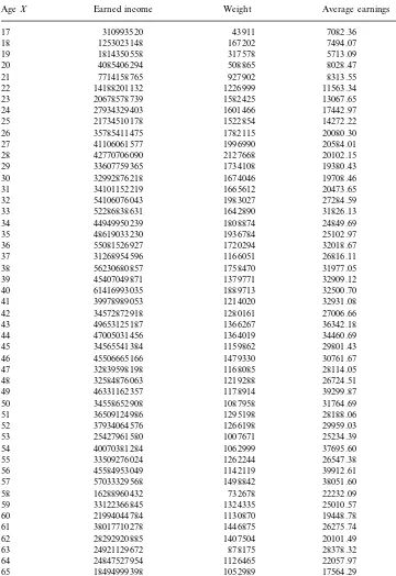
Using the magnetic tape of the 1983 FRB sample survey and the technical manual and code book prepared by Avery and Elliehausen (1988), we obtain, by age of the household head, (i) the households earned income; (ii) the weight each household represents in the U.S. population; and (iii) the average household earnings. These data are presented in Table 2.
Table 2
1983 U.S. household earned income by age of the head
Table 2 (Continued)
Average earnings
AgeX Earned income Weight
1116291
66 11036390439 9886.66
1204940 6276.71
7563060639 67
68 6512401439 1015925 6410.32
9059401881
69 968090 9358.02
70 3440934512 948991 3625.89
873677 9389.24
8203166986 71
72 1227720784 728488 1685.30
2793751660 1008679
73 2769.71
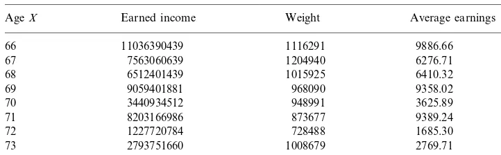
Because the maintenance cost c(x) is not considered, columns 4 and 5 of Table 3 present the level of gross HC by age at 6 and 8% discount rates, respectively, and because we did not make any assumption of productivity change by age, we call them ‘cross-section’ HC estimates. Therefore, to estimate the average household HC at agex, the average earnings of this representative household,tyears later, is assumed to be the average earnings of the households of agex+t.
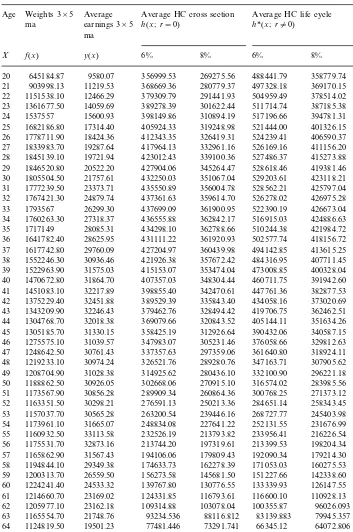
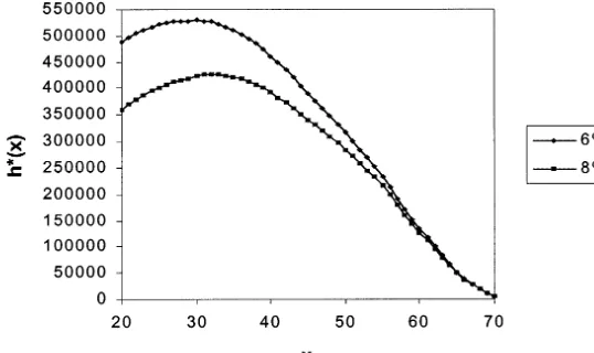
To obtain the life cycle HC estimation of the representative household by age of the head, we apply Eq. (15), where r stands for the annual rate of productivity growth. We assume thatr=0.03 for 205x529, because of the more intensive HC formation in this interval of age;r=0.02 for 305x554;r=0.01 for 555x564; and r=0 for x]65. The gross values of the average life cycle HC by age of the household head, for i=0.06 and 0.08, are presented in Fig. 3, and in Table 3, column 6, and 7.
Applying Eq. (14) to columns 4 and 5 of Table 3 and using the weights given in column 2, we obtain the 1983 U.S. average household HC, i.e. the cross-section averages,
A6HC(h)=$283 313, for i=0.06 and r=0; (20a)
A6HC(h)=$238 703, for i=0.08 and r=0; (20b)
The 1983 U.S. FRB sample survey gives the following average household wealth (Dagum, 1994),
A6K=$92 028.
Applying Eq. (16) to columns 6 and 7 of Table 3 and using the weights given in column 2, we obtain the estimates of the average life cycle HC of a 20 years old U.S. household head in 1983, i.e.
A6HC(h*)=$364 869, for i=0.06 and r"0; (21a)
A6HC(h*)=$303 336, fori=0.08 and r"0. (21b)
Table 3
1983 U.S. household human capital by age of the head (present values at 6 and 8% discount rates) Age Weights 3×5 Average Average HC cross section Average HC life cycle
h*(x;r"0)
20 645184.87 9580.07 356999.53 269275.56 488441.79 358779.74 368669.36 280779.37 497328.18 369170.15
1682186.80 405924.33 319248.98 521444.00 401326.15 25
1833983.70 417964.13 332961.16 526169.16 411156.20 27
28 1845139.10 19721.94 423012.43 339100.36 527486.37 415273.88 427904.06 345264.47 528618.46
1767421.30 437361.63 359614.70 526278.02 426975.28 32
1760263.30 436555.88 362842.17 516915.03 424886.63 34
28085.31
1717149 434298.10 362788.66 510244.38 421984.72 35
431111.22 361920.93 502577.74
28625.95 418156.72
36 1641782.40
29760.09
1617742.80 427204.97 360439.98 494142.85 413615.25 37
1470672.80 407357.03 348304.44 460711.75 391942.60 40
41 1451083.10 32217.89 398855.40 342470.61 447761.36 382877.53 389529.39 335843.40 434058.16
1305185.70 358425.19 312926.64 390432.06 340587.15 45
1248642.50 337357.63 297359.06 361640.80 318924.11 47
30974.24
1219233.10 326521.76 289280.76 347163.71 307905.62 48
314925.62 280436.10 332100.90
31028.38 296221.18
49 1208704.90
30926.05
1188862.50 302668.06 270915.10 316574.02 283985.56 50
1157037.70 263200.54 239446.16 268727.77 245403.98 53
248834.08
54 1173961.10 31665.07 227641.22 252131.55 231676.99 232526.19 213793.82 233956.41
1194844.10 174633.73 162278.39 171053.03 160275.53 58
1224241.40 139767.80 130776.55 133339.93 126147.55 60
1214660.70 23169.02 124331.85 116793.61 116600.10 110928.13 61
109314.88 103078.04 100355.87
23162.18 96026.093
62 1205977.10
21748.76
1165554.70 93234.536 88116.812 83139.883 79945.357 63
77481.446
64 1124819.50 19501.23 73291.741 66345.12 64072.806 62969.106 59521.144 50874.56
15956.31 49320.06
Table 3 (Continued)
Weights 3×5 Average Average HC life cycle
Age Average HC cross section
h*(x;r"0) ma earnings 3×5 h(x;r=0)
ma
8% 6%
y(x) 6% 8%
X f(x)
12796.08 51193.525 48334.018 38023.44 37016.188 66 1083580.30
41916.582 39526.982 27539.455
67 1075272.10 9841.40 26938.753
19374.914 33111.415
35114.252 19070.453
8004.14 68 1041606.30
6812.69 29765.067 28086.203 12484.341 12379.31 69 986735.40
6248.6197 23879.844 6248.6197
70 938314.60 6248.62 25287.276
Fig. 1. 1983 U.S. observed and smoothed (3×5 ma) household earned income by age of the head.
Fig. 3. 1983 U.S. household human capital by age of the head with productivity increase (life cycle) (at 6 and 8% discount rates).
Jorgenson and Fraumeni’s full (market and non-market) human and non-human wealth estimates are incommensurable with ours because of these authors’ inclusion of the non-market accounts with the scope of providing ‘‘a comprehensive perspec-tive on the role of capital formation in U.S. economic growth’’ (Jorgenson and Fraumeni, 1989). The incommensurability is strongly influenced by the authors’ very high values of the non-market labor income estimations, which are almost five times the market labor income estimations (see Jorgenson and Fraumeni, 1989 Tables 5.13 and 5.14), and the authors’ full labor income estimations for the period 1948 – 1984, which are between nine and 14 times the full property income (see Jorgenson and Fraumeni, 1989 Tables 5.15 and 5.16). This large fluctuation in the full labor/full property income ratio should be imputable to the method of estimating the households non-market labor outlays and labor incomes. Should this be the case, the assumptions leading to these estimations would require a thorough reassessment.
Jorgenson and Fraumeni provided a valuable and original contribution by incorporating the non-market activities and offering an ingenious approach to their estimations. Our observations and comments purport to point out the need of reassessing and refining their approach. Our observations are further supported by the following 1982 household averages obtained from Jorgenson and Fraumeni’s Table 5.32, for a population of household equal to 83 918 000,
1. the 1982 U.S. average of the full (market and non-market) household non-hu-man wealth is equal to $165 494;
2. the 1982 U.S. average of the full (market and non-market) household human wealth is equal to $1 989 924.
Frau-meni’s full human wealth estimation in 1982 is 556% (i.e. 6.56 times) higher than our 1982 average household market human wealth. Can this huge difference be imputable to the non-market human wealth? Jorgenson and Fraumeni’s contribu-tion does not provide enough informacontribu-tion to answer this quescontribu-tion. Besides, their full average household human wealth estimations for the period 1948 – 1984 are so high that, for a moderate level of human wealth inequality and rate of return, it would imply the practical inexistence of poverty or a very high percentage of HC idle capacity. In effect, at a reasonable 8% rate of return, the 1982 average full household human wealth of $1 989 924 would give an average household earned income of almost $160 000!
The estimations of Kendrick, (1976) regarding non-human and human wealth end in 1969. Using Jorgenson and Fraumeni’s rate of growth Kendrick’s 1969 estimations of the non-human and human wealth extrapolated to 1982 give $77 544 and $135 883, respectively. These estimations represent an 84.3% of the observed 1983 U.S. FRB average household non-human wealth, and a 44.8% of our life cyle average household human wealth estimation, using the 8% discount rate.
Macklem’s (1982) estimations for Canada, are,
(i.a) per capita non-human wealth in Canadian dollars of 1986 is equal to Can$40 906;
(ii.a) per capita human wealth in Canadian dollars of 1986 is equal to Can$238 043.
For a 3.2 average Canadian household size, we have,
(i.b) average household non-human wealth in Canadian dollars of 1986 is equal to Can$130 899;
(ii.b) average household human wealth in Canadian dollars of 1986 is equal to Can$761 738.
Taking into account the Canadian’s rate of inflation from 1982 to 1986 and the 1982 Canadian – U.S. exchange rate, we obtain an average household non-human wealth marginally higher than the U.S. while the Canadian average household human wealth is about twice our estimate for the US. There is not a good reason to account for so large difference. Besides, from 1963 to 1994, Macklem’s estima-tions present large, unacceptable and unsubstantiated fluctuaestima-tions. For instance, from 1963 to 1975, the human wealth estimations show an increasing trend followed by a decreasing trend until 1984, then an increasing one until 1988, then decreasing until 1990, followed by an increasing trend. Besides, the maximum human wealth estimation is obtained in 1988, which is very close to the 1975 estimation. These unbecoming fluctuations for an economy presenting a steady economic growth trend should be imputed to the limitations of the exogenous variables specified in the bivariate autoregressive model.
6.2.Estimation of HC of each sample obser6ation and its size distribution
household head;x6, years of schooling of the spouse; x7, number of children; x8, years of full-time work of the household head; x9, years of full-time work of the spouse;x10=k, total wealth; andx11=u, total debt. Hence, the latent variablezin Eq. (10) is specified as a linear function of qualitative and quantitative variables. Applying an iterative algorithm to estimate a latent variable as in Wold (1982) partial least squares and Dagum and Vittadini (1996), further developed by several authors to deal with the specification of qualitative and quantitative variables as in Young et al. (1976), Haagen and Vittadini (1998), Vittadini (1999), we obtain the following estimation ofzi, i=1, 2, …, 4103, where the numbers in parentheses are the Student-t:
zi= −0.222x1i−
(−1.3) 0.267(−25.1)x2i+0.115(6.0)x3i−0.087(−5.2)x4i+0.334(31.9)x5i+0.570(29.5)x6i +0.045x7i
(3.6) +0.042(2.6)x8i−0.088(−7.6)x9i+0.090(8.3)x10i+0.154(14.7)x11i; (22) wherezi andxij,j=1, 2, …, 11, are standardized variables. The corresponding R
2
andF values are,
R2
=0.618 and F(11, 4091)=602.9.
Given that we are working with a cross-section sample of 4103 observations, the coefficient of determination R2 and the F value are exceptionally high, hence, clearly accepting the goodness of fit of Eq. (22) even at the 1% level of significance. In effect, at the 5 and1% significance levels, theFcritical values with 11 and 4091 degrees of freedom are 1.31 and 2.30, respectively.
Applying the transformation (Eq. (11)) to the estimations ofziin (Eq. (22)), we obtain the accounting monetary estimations of hi, i=1, 2, …, 4103, each one having a weight that corresponds to the number of households each sample observation represents in the 1983 U.S. population. Dividing each hi by its mean obtained from Eq. (12) and multiplying by the average household HC given by Eq. (20a) or Eq. (20b), we obtain the household HC distribution in US dollars, with mean equal to $283 313, if the flow of average earnings is actualized at 6%, or with mean equal to $238 703, if it is actualized at 8% discount rate.
6.3.Fitting the household HC distribution
Applying the non-linear least squares method of parameters estimation, the sample estimation (data) of the household HC distribution at 8% discount rate are fitted to Dagum three- and four-parameter model given in Eqs. (18) and (19). The fitted three-parameter model Eq. (18) is,
F(h)=(1+3146.48h−2.3421 )−0.4101
, h\0, (b,l)\0, SSE=0.00199,
K-S=0.039, (23)
whereas for the four-parameter model (Eq. (19)), we have,
F(h)= −0.0762+1.0762(1+3134.81h−2.2929)−0.341,
h\h0]0,
wherehis measured in $10 000, SSE stands for the sum of the squares errors,K–S
for the Kolmogorov – Smirnov statistic, and h0 is the solution of F(h)=0 in Eq. (24), i.e.
h0=l1/d
1− 1 a1/b
−1
n
−1/d
=1.1326. (25)
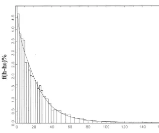
The HC histogram and its fitted probability density function corresponding to the estimated four-parameter Dagum model (Eq. (24)) are presented in Fig. 4, which shows further evidences of its excellent goodness of fit.
The asymptotic critical value of the K–S statistic at 10, 5, and 1% significance levels are K–S(0.10)=1.22/41031/2
=0.019, K–S(0.05)=1.36/41031/2
=0.021, and
K–S(0.01)=1.63/41031/2
=0.025, respectively. Hence, according to this approxi-mated criterion to test the goodness of fit, the four-parameter fitted model clearly accepts it whereas the three-parameter does not. We call it approximated criterion or a proxy test because we are working with the fitted model instead of an independently specified distribution, hence the significance level should be larger than in the case of two independently observed or specified distributions. The goodness of fit of the four-parameter model continues to be accepted even at the 10% significance level because of its very lowK–S statistic.
A way to test if there is a statistically significant reduction in the SSE, when passing from the three- to the four-parameter model, makes use of theF-test. Since we have one extra parameter and we fit both models to the HC data grouped in 47 class intervals, we have 42 degrees of freedom for the four-parameter model. Therefore,
F(1, 42)=(0.00199−0.00075) (0.00075/42) =69.5,
whereas the critical level at 5% significant level isF0.05(1, 42)=4.07. Hence, the null hypothesis that the four-parameter model does not significantly reduce the SSE of the three-parameter fitted model is strongly rejected.
Since the estimate of a is significantly different from zero, and is negative, the estimated model (Eq. (24)) is Dagum type III. Translating the ordinate to the point
h0=1.1326, we have,
F(h)=[1+3134.81(h−1.1326)−2.2929]−0.341,
h\1.1326. (26)
The solution F(h)=0.5 in Eq. (24) is the estimated median of the fitted distribution. It is equal to $163 539 whereas the median of the sample values ofh
is equal to $163 061, i.e. the model estimation and the sample value of the median are almost identical, further supporting the goodness of fit of Eq. (24). The mathematical expectation (the estimated mean) is equal to $255 367 and the sample mean is equal to $238 703, presenting a discrepancy of less than 7%.
The Gini ratio is G=0.528, which is smaller than the Gini ratio for the total wealth (G=0.636) and for the net wealth (G=0.681), and greater than the income inequality (G=0.444), which are estimated from the same household sample survey (Dagum, 1994).
7. Conclusion
The method of HC estimation proposed in this study makes a fruitful combina-tion of the latent variable methods of estimacombina-tion and the prospective method developed by Farr (1853).
The issue of obtaining accurate estimates of the expected flow of earned incomes by age is solved when working with sample surveys of income and wealth distributions, i.e. because of their large sizes, the law of large numbers applies.
Our HC estimation is compared with the best known HC estimates done in the last quarter of the 20th century, i.e. those obtained, for the US by Jorgenson and Fraumeni (1989) and by Kendrick (1976), and for Canada, by Macklem (1997). According to our recollection, it is the first time that the size distribution and model estimation of HC is done working with a sample survey of income and wealth distribution, thus enlarging the frontier of income and wealth research.
Basic contributions to the field of endogenous growth theory that incorporate the concept of HC were done by Romer (1986), Lucas (1988). Dagum (1978, 1980) introduced the IGF model as a function of HC and wealth; Dagum (1994) specified an IGF model as an equation in a causal model of income, HC, and wealth determination; and in Dagum (1998, 1999) it became a basic equation to link the functional and the personal income distributions, and to support the design of socioeconomic policies of growth with social equity. Besides, the proposed method of estimating the HC and its distribution among a population of economic units can be highly relevant to make further advances in the development of endogenous growth theory.
The method developed and applied in this research and the statistical information provided by the consumer finances and the employment and unemployment sample surveys, hopefully enlarged with some additional questions, can be fruitfully applied to estimate the human capital of the members of the labor force, to investigate its HC structure and distribution, to analyze the amount of idle HC, the unemployment rate of the labor force, and the main types of unemployed HC. These themes should be essential parts of any future socioeconomic research program of growth and development.
Acknowledgements
We thank an anonymous referee for his/her helpful comments on an early version of this paper. Research grant no. 9713037571001 from the Ministry of the Univer-sities and of Scientific and Technological Research (MURST) is gratefully acknowl-edged.
References
Azariadis, C., Drazen, A., 1990. Threshold externalities in economic development. Q. J. Econ. 105 (2), 501 – 526.
Avery, R.B., Elliehausen, G.E., 1988. 1983 Survey of Consumer Finances: Technical Manual and Codebook. U.S. Federal Reserve System, Washington, DC.
Barriol, A., 1910. La valeur sociale d’un individu. Revue Economique Internationale 552 – 555. Barro, R.J., 1991. Economic growth in a cross section of countries. Q. J. Econ. 106 (2), 407 – 443. Becker, G.S., 1962. Investment in human capital: a theoretical analysis. J. Political Econ. LXX (5),
9 – 49.
Becker, G.S., 1975. Human Capital, second ed. Columbia University Press and NBER, New York. Beneluce, A., 1904. Capitali sottratti all’Italia dall’emigrazione per l’estero. Giornale degli Economisti
2a. Serie Anno XV XXIX, 506 – 518.
Cantillon, R., 1755. Essay sur la nature du commerce en ge´ne´ral. Reprinted for Harvard University, Boston, p. 1892.
Dagum, C., 1977. A new model of personal income distribution: specification and estimation. Economie Applique´e XXX (3), 413 – 436.
Dagum, C., 1980. The generationa and distribution of income, the Lorenz curve and the Gini ratio. Economie Applique´e XXXIII (2), 327 – 367.
Dagum, C., 1983. Income distribution models. In: Kotz, S., Johnson, N.L. (Eds.), Encyclopedia of Statistical Sciences, vol. 4. Wiley, New York, pp. 27 – 34.
Dagum, C., 1994. Human capital, income and wealth distribution models and their applications to the USA, Proceedings of the American Statistical Association, Business and Economic Section, pp. 253 – 258.
Dagum, C., 1996. A systemic approach to the generation of income distribution models. J. Income Distributions 6 (1), 105 – 126.
Dagum, C., 1998. Fondements de bien-e´tre social et de´composition des mesures d’ine´galite´ dans la re´partition du revenu, Tenth Invited Lecture in Memory of Franc¸ois Perroux, Colle`ge de France. Economie Applique´e LI (4), 151 – 202.
Dagum, C., 1999. Linking the functional and personal distribution of income. In: Silber, J. (Ed.), Handbook of Income Inequality Measurement. Kluwer Academic Publishers, Hingham, MA, pp. 101 – 128.
Dagum, C., Vittadini, G., 1996. Human capital measurement and distributions, Proceedings of the Business and Economic Statistics Section, American Statistical Association, pp. 194 – 199.
de Foville, A., 1905. Ce que c’est la richesse d’un peuple. Bullettin de l’Institut International de Statistique XIV (3), 62 – 74.
Denison, E.F., 1967. Why Growth Rates Differ. The Brookings Institute, Washington, DC.
Denison, E.F., 1974. Accounting for United States Economic Growth 1929 – 1969. The Brookings Institute, Washington, DC.
Dublin, L.I., Lotka, A., 1930. The Money Value of Man. Ronald, New York.
Eisner, R., 1978. Total income in the United States 1959 and 1969. Rev. Income Wealth 24 (1), 41 – 70. Engel, E., 1883. Der Werth des Menschen. Verlag von Leonhard Simion, Berlin.
Farr, W., 1853. Equitable taxation. J. R. Stat. Soc. XVI, 1 – 45.
Ferrari, G., 1932. Il costo monetario dell’uomo, Atti del Secondo Congresso Internazionale per gli studi sulla popolazione, Roma.
Fisher, I., 1927. The Nature of Capital Income. Macmillan, London. Gibrat, R., 1931. Les ine´galite´s e´conomiques. Sirey, Paris.
Gini, C., 1931. Le basi scientifiche della politica della popolazione. Studio Editoriale Moderno, Catania. Gini, C., 1954. Patologia Economica, fifth ed. UTET, Turin.
Haagen, K., Vittadini, G., 1998. Restricted regression component decomposition. Metron LVI (1 – 2), 53 – 75.
Jorgenson, D.W., Fraumeni, B.M., 1989. The accumulation of human and nonhuman capital, 1948 – 84. In: Lipsey, R.E., Stone Tice, H. (Eds.), The Measurement of Saving, Investment, and Wealth, NBER Studies in Income and Wealth, vol. 52. The University of Chicago Press, Chicago, pp. 227 – 282. Kendrick, J.W., 1976. The Formation and Stocks of Total Capital. Columbia University Press, New
York.
Laroche, M., Me´rette, M., 1999. Measuring human capital in Canada, Research Paper. Department of Finance, Ottawa, Canada.
Lau, L., Dean, J., Jannison, T., Louat, F., 1991. Education and productivity in developing countries: an aggregate production function approach. In: Policy and Research Working Paper, WPS 612. World Bank, Washington, DC.
Lucas, R.E., 1988. On the mechanics of economic development. J. Monetary Econ. 22 (1), 3 – 42. Machlup, F., 1962. The Production and Distribution of Knowledge in the United States. Princeton
University Press, Princeton, NJ.
Macklem, R.T., 1997. Aggregate wealth in Canada. Can. J. Econ. 30 (1), 152 – 168.
Mandelbrot, B., 1960. The pareto-le´vy law and the distribution of income. Int. Econ. Rev. 1, 79 – 106. Mandelbrot, B., 1963. New methods in statistical economics. J. Political Econ. LXXXI (5), 421 – 440. Mankiw, N.G., Romer, D., Weil, D.N., 1992. A contribution to the empirics of economic growth. Q. J.
Econ. 107 (2), 407 – 437.
Marshall, A., 1922. Principles of Economics. Macmillan, New York.
Mincer, J., 1970. The distribution of labor incomes: a survey. J. Econ. Literature VIII (1), 1 – 26. Mortara, G., 1934. Costo e rendimento economico dell’uomo, Atti dell’Istituto Nazionale delle
Assi-curazioni, vol. VI, Roma.
Mulligan, C.B., Sala-i-Martin, X., 1997. A labor – income-based measure of the value of human capital: an application to the states of the United States. Jpn. World Econ. 9 (2), 159 – 191.
Nehru, V., Swanson, E., Dubey, A., 1995. A new database on human capital stock in developing and industrial countries: sources, methodology, and results. J. Dev. Econ. 46, 379 – 401.
Nicholson, J.S., 1891. The living capital of the United Kingdom. Econ. J. I (1), 95 – 107. Nordhaus, W.D., Tobin, J., 1972. Economic Growth. NBER, New York.
Pareto, V., 1895. La legge della domanda, Giornale degli Economisti, pp. 59 – 68.
Pareto, V., 1896. Ecrites sur la courbe de la richesse. Oeuvres Comple`tes de Vilfredo Pareto publie´es sous la direction de G.H. Bousquet et G. Busino. Librairie Droz, Gene´ve, p. 1965.
Pareto, V., 1897. Cours d’e´conomie politique, Nouvelle Edition publie´e sous la direction de G.H. Bousquet et G. Busino. Librairie Droz, Gene´ve, p. 1964.
Pareto, V., 1905. Il costo economico dell’uomo ed il valore economico degli emigranti. Giornale degli Economisti, 2a. Serie, Anno XVI XXX, 322 – 327.
Perroux, F., 1974. Le e´conomie de la ressource humain. Mondes en de´velopment 7, 17 – 81.
Petty, W., 1690. Political Arithmetick, reprinted in C.H. Hull, The Economic Writings of Sir William Petty.
Pietra, G., 1931. In: Casagrandi, O. (Ed.), Importanza sociale ed economica delle epidemie, Trattato italiano d’igiene. UTET, Torino.
Psacharopoulos, G., Arriagada, A.M., 1986. The educational composition of the labor-force: an international comparison. Int. Labor Rev. 125 (5), 561 – 574.
Ricardo, D., 1817. Principles of political economy, New edition by Piero Sraffa: Works and Correspon-dence of David Ricardo, Cambridge University Press, Cambridge, p. 1951.
Romer, P.M., 1986. Increasing returns and long-run growth. J. Political Econ. 94 (5), 1002 – 1037. Romer, P.M., 1989. Human Capital and Growth: Theory and Evidence, NBER Working Paper, N.
3173.
Ros Jimeno, J., 1931. Valor Economico del Hombre, Proceedings of the XXth Session of the International Statistical Institute.
Rutherford, R.S.G., 1955. Income distribution: a new model. Econometrica 23 (3), 277 – 294. Smith, A., 1776. The Wealth of Nations. The Modern Library, New York.
Schultz, T.W., 1959. Investment in man: an economist’s view. Soc. Sci. Rev. XXXIII (2), 109 – 117. Schultz, T.W., 1961. Investment in human capital. Am. Econ. Rev. LI (1), 1 – 17.
Sensini, G., 1908. Il metodo ordinario nel calcolo del costo di produzione dell’uomo. Giornale degli Economisti XXXVI, 481 – 496.
Vittadini, G., 1999. Analysis of qualitative variables in structural models with unique solutions. In: Vichi, M., Opitz, O. (Eds.), Classification and Data Analysis, Theory and Application. Springer, Berlin.
Wittstein, T., 1867. Mathematische Statistik und deren Anwendung auf National-Okonomie und Versicherung-wiessenschaft. Hahn’sche Hofbuchland-lung, Hanover.
Willis, R.J., 1986. Wage determinants: a survey and reinterpretation of human capital earnings fucntions. In: Ashenfelter, O., Layard, R. (Eds.), Handbook of Labor Economics, vol. I. Elsevier, New York, pp. 525 – 602.
Wold, H., 1982. Soft modeling: the basic design and some extensions. In: Joreskog, K.G, Wold, H. (Eds.), Systems Under Indirect Observation: Causality, Structure, Prediction, vol. 2. North-Holland, Amsterdam, pp. 1 – 54.
Young, F.W., De Leeuv, J., Takane, Y., 1976. Regressions with qualitative and quantitative variables: an alternating least squares method with optimal scaling features. Psychometrika 41 (4), 505 – 529.