Lieke et.al. Pollutant Dispersion in Some Fishing
POLLUTANT DISPERSION IN SOME FISHING COAST AREAS
OF EAST JAVA INDONESIA
Lieke RiadP· Ali Altway
21Chemical Engineering Department, University ofSurabaya, Surabaya, Indonesia 2Chemical Engineering, lnstitut Teknologi Sepuluh Nopember, Surabaya, Indonesia
Email : [email protected]
Abstract: The existence of pollutant in some coastal areas in Muncar has drawn attention from local government. The indicator of the existence of pollutant was measured as Chemical Oxygen Demand (COD), Total Suspended Solid (TSS), N-ammonia, and Fat and Oils. There are several fishery industries located nearby the coast. Sample were taken from the outlet discharge of several industries in three coastal areas which are located close each other in each cluster. The discharge of waste water from several industries which the samples taken flows to each river in each cluster. This paper reported. pollutant dispersion model in three rivers, named Kalimati, Kali Tratas,and Irigasi. Results showed that the rate of dispersion in irigasi river is the fastest compared to two other rivers. It took 2000 seconds for the COD and TSS to disappear at I 00 meters length distance, while it took 2000 seconds for N-ammonia and Fat and Oils to disappear at 60 meters length distance from the discharge spot in irigasi river. There is about 24.500 seconds for COD, TSS, N-ammonia and Fat and Oils to disappear at the distance of200 meters length and 4 meters width from the discharge spot in Kali Tratas. It also took about 24.500 seconds for COD, TSS, N-ammonia and Fat and Oils to disappear at the distance of 200 meters length and 2.4 meters width from the discharge spot in Kalimati.
Keyword: pollutant dispersion, muncar, fishery industry, waste water.
Abstrak: Keberadaan pantai muncar yang tercemar telah menarik perhatian pemerintah local. Indikator yang dapat menunjukkan adanya pencemaran tersebut ditunjukkan dengan nilai Chemical Oxygen Demand (COD), Total Suspended Solid (TSS), N-ammonia, and Fat and Oils. Ada beberapa industri perikanan yang terletak dekat dengan posisi pantai Muncar, Sampel diambil dari beberapa keluaran pembuangan limbah dari beberapa industri yang letak keluaran pembuangan sang at berdekatan di tiga area pantai. Keluaran limbah dari beberapa industri yang diambil mengalir ke sungai yang ada di masing-masing cluster. Tulisan ini menunjukkan model dispersi polutan di tiga sungai yaitu Kalimati, Kali Tratas dan sungai irigasi. Hasil simulasi menunjukkan laju dispersi di sungai irigasi adalah yang tercepat dibandingkan dengan laju dispersi di dua sungai yang lain. Waktu yang dibutuhkan untuk konsentrasi COD dan TSS mencapai nilai 0 ppm , pada jarak I 00 meter ke arah axial dari sumber pembuangan di sungai irigasi adalah 2000 detik. Dibutuhkan waktu yang sama untuk kandungan N-ammonia, minyak dan lemak yang ada di sungai irigasi mencapai nilai 0 ppm,padajarak 60 meter dari sumber pembuangan di sungai irigasi. Dibutuhkan 24500 detik untuk membuat konsentrasi COD,TSS, N-ammonia, minyak dan lemak mencapai 0 ppm di Kali Tratas padajarak 200 meter panjang sungai dan 4 meter Iebar sungai dari sumber pembuangan. Sedangkan, untuk Kalimati, dibutuhkan waktu 24500 detik untuk konsentrasi COD, TSS, N-ammonia, minyak dan lemak untuk mencapai 0 ppm, pada jarak 200 meter panjang sungai dan 2.4 meter Iebar sungai dari sumber pembuangan limbah.
Kata kunci: dsipersi polutan, muncar, industri perikanan, air limbah industri.
INTRODUCTION
There are several coast areas in Banyuwangi that have been identified as famous fishery indus-tries in East Java, Indonesia. There are around
130.000 inhabitants in the area. There are many fish processing industries which were located in several villages along the coast that connected to Bali Strait. The coast area is called Muncar. It was noted that those are around 70 big fishery indus-tries and hundred horne fishery indusindus-tries. The ac-tivity of those big industries are fish flour
process--A ing, cold storage, fish oil and fish cannery. The
) small industries produce fish fermented paste and
10
INDUSTRI ISSN 1693·0533
for waste water from home fish industries. The river which was visited are Kalimati, Irigasi, and Kali Tratas. The dimension in width and depth ofKali Tratas, Kalimati, Irigas rivers are 20 m x 1 m; 12 m x 1 m; 1.5 mx 0.8 m consecutively. The samples taken from several industries which are closed to the three rivers. The flow rate ofthe waste water discharged to the Kalimati river is 5200 m3/day, to the Tratas river is 500 ffil/day and to the Irigasi river is 3560 m3/day, there is about 5740 m3/day of waste water discharged to the sea which was not taken for the observation.
THEORY
The Dispersion Process
The two dimensional model (Figure 1) is used because we need to predict the mixing relatively close to the source which is concentrated at one bank, and to predict the depth-average concen-tration anywhere in the cross section. The two dimension model, depth-average equation is :
ィセKA⦅HィオcI@
at
ax
KセHィキcI@
ay
=
セHィ・Z@
ac)
+
セ@
(
h
Eac)
ax
Xax
ay
y ay
(1)
£y= 0.23 u
*
h;u= linear (longitudinal) velocity of the river stream ( LT1
); h =depth of the river (L); c= empirical mixing coefficient (U T1
); w =transverse velocity (LT1
)
ex=
5.93 u*
hp
= HᆪクNセエIOHセクI R@ has to be less than 0.5'Y= HᆪケNセエIOHセケI RL@ 'Y has to be less than 0.5
8y =Lin, L =width of the river y
p,
'Y =non-uniform velocity distribution coefficient/!:,x = distance between two computational points
in x-direction
8y= distance between two computational points in y-direction
The source ofthe waste water is modeled as a tracer which is injected instantaneously, then the idispersion equation is assumed to be ofthe form:
-Vol.11 No.1 : 10-14
y
t
X·Figure 1. Two dimensional model
+/!:,t =time between two computational intervals n =number of increment in y-direction y
a
a
at
(ACa)
+ox
(AUCa)
=セ@
(AK oca)
OX X OX
(2)
K
:e=
longitudinal mixing coefficient= 12.5 h. u (UT1)
Ca.= cross sectional average concentration(ML-3 ) U=cross sectional average velocity (LT1
) A= flow area (U)
The Convection Process
The convection which is expressed for the flow area A and for steady flow is
oACa
+
a(AUCa) =O (3)at
a:e
Some finite difference approximations to equation (3) represent a different equation ,
a ca.
+
U a ca. = K a.,.caot
a:e
na:e'li
a=0.258x
Kn<Kx
oc(.ax-a)
Kn=
---'---'-2dt
a = factor if /!:,x
"t
U 8tKn =artificial diffusion coefficient (L2T1 )
(4)
Kx =longitudinal dipersion coefficient (UT1 ) (M = mass, L= length, T= time)
A two dimensional model based on equation
(1) could be developed by writing a fmite difference algorithm to solve for convection and diffusionin the longitudinal (x) and transverse diffusion (y direction). By assuming the steady river flow conditions, the transverse·velocity w is small compared to the longitudinal velocity u. The river
Lieke et.al.
is divided into a series of adjacent stream tubes, in each the discharge is constant, steady river flow condition is used as assumption. An algorithm was
developed which stimulates two dimensional
mix-ing as the simultaneous occurrence of three
mecha-nisms, 1) longitudinal convection in each stream
tube, 2) longitudinal diffusion in each stream tube, 3) transverse diffusion between adjacent stream tubes (2 ), since the quasi-two-dimensional model recognizes only an average concentration in each stream tube. The resulting expression is :
oc a o ( oc)
A-+-(AuC) = - AE -
-{}t OX OX X OX
ac
ac
(5)(hEy ay)l + (hEy ay)r
the finite difference solution in equation ( 5) is done by dividing the river into a series of computational reaches separated by computational points.
Longitudinal Convection
It is calculated in each stream tube from its
upstream limit to its downstream limit. For pure convection, the equation is written :
A ac
+
a (Auc) = 0ar: ax (6)
The velocity in each one is different, セエ@ and セク@ will
be the same for all tubes
Longitudinal Diffusion
This diffusion proceeds in each stream tube from upstream to downstream boundary. The equation
IS:
A ac
=
セ@(
A £. !£..}ot
ax
Xax
(7)Transverse Diffusion
This diffusion occurred between stream tubes and along their entire length is calculated using :
oc
oc
oc
A-= -(hE -)l+(hE -)
Ot y Oy y Oy T (8)
Based on equation ( 1 ), which describes tracer mass
conservation at a point, must be integrated over the width of a stream tube, since the quasi two dimensional model which is proposed recognizes only an average concentration in each stream tube.
12
-Pollutant Dispersion in Some Fishing
The resulting expression is the following :
ac
a
a (
ac)
A-+ - (AuC)
= -AE -
-at ax
ax
Xax
ac
ac
(hEy ay)z
+ (
h
fya)r
(9)
MATERIALS AND METHODS
Samples were taken from the sampling points at the end of pipeline for waste water eftluent discharged from several industries which flow to Kalimati, Tratas and Irrigasi rivers. The samples were mixed for each river and analysed for Chemical Oxygen Demand (COD), TSS (Total Suspended Solid), N-ammonia, Fat and Grease. All samples were preserved prior laboratory analysis. COD was measured using closed reflux, colorimetric method, TSS was measured by dry weight method. N-ammonia was measured by titrimetric method (I), whereas Fat and Grease was measured using soxhlet extraction method ( 1 ). The dispersion ofpollutant is simulated using two-dimensional dispersion modeling using MATLAB. The two dimensional dispersion consider three mechanisms : 1) longitudinal convection; 2) longitudinal diffusion; 3) transverse diffusion. We used three mechanisms for pollutant dispersion in Kalimati and Kali Tratas, whereas we used two mechanisms (longitudinal convection and longitudinal di:Jfusion) for irigasi river.
RESULTS AND DISCUSSION
The characteristics and flow rate of waste water to each river is shown in Table 1.
INDUSTRI ISSN 1693-0533
nver.
Table 1. Characteristics of waste water discharged Kali Kalimati Irigasi Tratas
Initial COD,ppm 4320 8420 1200 Initial TSS,ppm 620 12430 595 Initial N-ammonia,ppm 60 3564 67 Initial Fat and Grease,ppm 952 41094 225 Flowrate ofriver, 0.398 0.11 0.1 nf/second
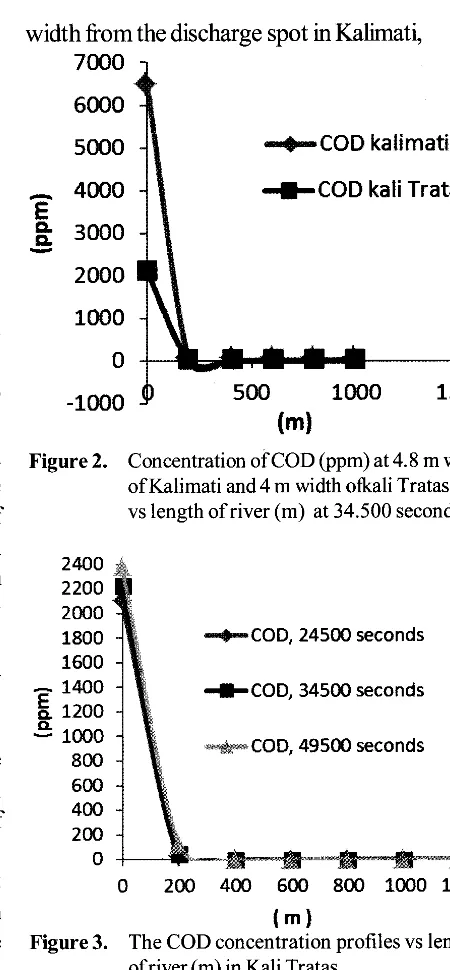
If we look at the Figure 2, the dispersion rate of COD inKalimati (at the position of4.8 m width) is slower compared to the distribution rate of COD in Kali Tratas (at the position of 4 m) for 34.500 seconds. It is due to the linear velocity in Kali Tratas is higher than that in Kalimati rivers. Figure 3 and Figure 4 showed the dispersion rate of COD, at different period were same both in Kalimati and Kali Tratas, which can be seen from the overlapping curve for concentration vs time profile. The same profiles occurred for TSS, N-ammonia, Fat and Oils both in Kalimati and Kali Tratas. Hence, the diffusivity for COD, TSS, N-ammonia Fat and oils in Kali Tratas were same, as well as that for Kalimati. Since the width ofthe irigasi river is not as wide kalimati and kali Tratas, the dipersion rate was simulated as a function of time and length of the river. At 2000 seconds, dispersion rate of COD, N-ammonia, TSS, Fat and Oils in Irigasi river were different for each pollutant with the highest dispersion rate was the COD dispersion rate and the lowest was Fat and Oils dispersion rate which can be seen in Figure 5. At 2000 seconds and 80 meters from the out-let discharge in Irigasi river, the COD concentra-tion has been reduced 94 %, which was from 334 ppm to 19.94 ppm. The TSS concentration has been reduced 94% from 166 ppm to 9.89 ppm. TheN -ammonia concentration has been re-duced 94 % from 19 ppm to 1.11 ppm, whereas the concentration ofF at and Oils has been reduced 94% from 63 ppm to 3.74 ppm
There is about 24.500 seconds for N-ammo-nia to disappear at the distance of 200 meters length and various position width from the 、ゥセᆳ
charge spot in Kali Tratas. It also took about 24.500 seconds N-ammonia to disappear at the idistance of200 meters length and various position
-Vol. 11 No. 1 : 10-14
width from the discharge spot in k。ャゥュ。エセ@
7000
-
E
a.. a..
-6000
5000
4000
3000
2000
1000
0
....,._COD kalimati
-COD kali Tratas
-1000 500 1000 1500
(m)
Figure 2. Concentration of COD (ppm) at 4.8 m width ofKalimati and 4 m width o1kali Tratas vs length of river (m) at 34.500 seconds
2400 2200 2000
1800 -+-COD, 24500 seconds 1600
-1400 [ 1200
セcodL@ 34500 seconds
..e:
1000800 セcodL@ 49500 seconds 600
400 200
0
+--__.,___ ". • •
% •0 200 400 600 800 1000 1200
( m)
Figure 3. The COD concentration profiles vs length ofriver(m) inKali Tratas
8000 7000 6000 -5000 [ 4000
c.
-3000 2000 1000
...,..COD, 24500 seconds ---COD, 34500 seconds
セcodL@ 49500 seconds 0 MャMMMMMMNMGヲゥャャMWBGQQQQセMキᄋセᄋャャャMMMセ@
0 500 1000 1500
( m)
Figure 4. The COD concentration profiles vs length of river (m) in Kalimati
[image:4.594.256.481.62.547.2] [image:4.594.254.477.67.279.2] [image:4.594.26.244.94.200.2])
Lieke et.al.
400 350 300 -250 [200
D..
-150 100 50 0
0 50
-.-coo
-TSS N-Ammonia
セf。エ@ and oil
100
( m)
[image:5.599.59.268.63.247.2]150
Figure 5. Concentration of pollutants vs length of river (m) at 2000 seconds in Irigasi river
-
3500 3000MッセMMカ]ッ@
2500
•••••• y=2.4 m
-2000 E
a. - - - y=4.8m
セ@ 1500
-+
y=7.2m 1000 -11- y=9.6m500 0
0 500 1000 1500
( m)
Figure 6. Concentration of N-ammonia profile vs length of river at various width of Kali Tratas river (y)
30
40
l
セG@
I
20 .c.
10
0 500
--1--•y=O
... y=4 m
- , - y=Bm
-+
·y=12 m••-Hi•• v= 16m
1000 1500
( m)
Figure 7. Concentration ofN-ammonia profilevs length of river at various width ofKalimati river (y)
セᄋ@ 14
-Pollutant Dispersion in Some Fishing
CONCLUSIONS
The pollutant dispersion model showed that the high concentration of COD, TSS, N-ammonia, Fat and Oils will be reduced to lower concentra-tion due to the diluconcentra-tion of river water which has a certain linear velocity. The dispersion model has been simulated using transverse diffusion and lon-gitudinal convection and lonlon-gitudinal diffusion model for both Kalimati and Kali Tratas . The dispersion model has been simulated using longi-tudinal convection and longilongi-tudinal diffusion model for irigasiriver. The dispersion rate of COD, TSS, N-ammonia, Fat and Oils at different period time were same both in Kalimati and Kali Tratas. The dispersion rate of COD, N-ammonia, TSS, Fat and Oils in I rigasi river were different for each pollutant with the highest dispersion rate was the COD dispersion rate and the lowest was the dis-persion rate of Fat and Oils.
REFERENCES
APHA. (1998). Standard methods for the examination of water amd waste water, 201
h ed., edited by L.S.Clesceri, A.E Greenberg, A.D. Eaton, p 361-363.
Cunge J.A, HollyF.M,Verwey A. (1980). Prac-tical Aspects of Computational River Hy-draulics. Pitman Advanced Publishing
Ltd.Boston, pp 312-340.
Czemuszenko , W . (1987) . " Dispersion of pollutants in rivers" ,Hydrological Sciences-,Vol
32, pp 59-67.
[image:5.599.40.506.266.781.2]