arXiv:1709.06071v1 [cs.GT] 18 Sep 2017
Managing Price Uncertainty in Prosumer-Centric Energy Trading:
A Prospect-Theoretic Stackelberg Game Approach
Georges El Rahi, S. Rasoul Etesami, Walid Saad, Narayan Mandayam, and H. Vincent Poor
Abstract— In this paper, the problem of energy trading be-tween smart grid prosumers, who can simultaneously consume and produce energy, and a grid power company is studied. The problem is formulated as a single-leader, multiple-follower Stackelberg game between the power company and multiple prosumers. In this game, the power company acts as a leader who determines the pricing strategy that maximizes its profits, while the prosumers act as followers who react by choosing the amount of energy to buy or sell so as to optimize their current and future profits. The proposed game accounts for each prosumer’s subjective decision when faced with the uncertainty of profits, induced by the random future price. In particular, the framing effect, from the framework of prospect theory (PT), is used to account for each prosumer’s valuation of its gains and losses with respect to an individual utility reference point. The reference point changes between prosumers and stems from their past experience and future aspirations of profits. The followers’ noncooperative game is shown to admit a unique pure-strategy Nash equilibrium (NE) under classical game theory (CGT) which is obtained using a fully distributed algorithm. The results are extended to account for the case of PT using algorithmic solutions that can achieve an NE under certain conditions. Simulation results show that the total grid load varies significantly with the prosumers’ reference point and their loss-aversion level. In addition, it is shown that the power company’s profits considerably decrease when it fails to account for the prosumers’ subjective perceptions under PT.
I. INTRODUCTION
One key enabler of smart grid energy trading and man-agement schemes is the presence of prosumers, i.e., smart grid customers capable of generating and storing their own energy. Indeed, the notable increase in penetration of solar photovoltaic (PV) panels and storage devices at the prosumer side of the grid will lead to novel demand-side energy management (DSM) schemes that will help alleviate the extremely expensive peak consumption hours and match consumption demand to the intermittent renewable energy supply of the grid [1].
A number of recent works [2]–[4] have studied the role of storage devices in grid energy management. For example, the authors in [2] propose a storage scheduling and management
Georges El Rahi and Walid Saad are with Department of Electrical and Computer Engineering, Virginia Tech, Blacksburg, VA email: (gel-rahi,walids)@vt.edu.
S. Rasoul Etesami and is with Department of Industrial Engineering, Uni-versity of Illinois at Urbana-Champaign, IL (email: [email protected]). Narayan Mandayam is with Department of Electrical Engineering, Rut-gers University, North Brunswick, NJ (e-mail: [email protected]). H. Vincent Poor is with Department of Electrical Engineering, Princeton University, Princeton, NJ (e-mail: [email protected]).
This research was supported in part by the NSF under Grants ECCS-1549894, ACI-1541105, ECCS-1549881, CNS-1446621, and ECCS 1549900.
model, with the goal of minimizing peak hour consumption. In [4], consumer-based storage scheduling is proposed in an attempt to match energy consumption to the expected power output of a central wind generation unit. In addition, the work in [3] studies the topic of optimal offerings for wind power generators, through the application of a common storage device. Moreover, the work in [5] adopts a stochas-tic optimization and robust optimization approach to study demand response for residential appliances under uncertain real-time prices.
Game-theoretic methods have been widely applied in the existing DSM literature, given the coupled interactions be-tween prosumers as discussed in [4], [6]–[10]. For instance, the authors in [6] propose a load scheduling technique with a dynamic pricing strategy related to the total consumption of the grid. More particularly, a number of works [7]–[10] have used the framework of Stackelberg games in order to study the hierarchical interactions between the power company and the grid’s consumers. For example, the authors in [7] propose a Stackelberg game approach to deal with demand response scheduling under load uncertainty based on real-time pricing in a residential grid. Similarly, the authors in [8] and [10] use a Stackelberg game approach between one power company and multiple users, competing to maximize their profits, with the goal of flattening the aggregate load curve. On the other hand, the authors in [9] propose a Stackelberg game approach between company and consumers, while studying the impact that a malicious attacker could have, through the manipulation of pricing data. In addition, the works in [11] and [12] have used a Stackelberg game approach to characterize the demand response of consumers with respect to the retail price. In particular, the authors adopted stochastic and robust optimization methods to study energy trading with uncertain market prices. Moreover, a Stackelberg game for energy sharing management of microgrids with photovoltaic prosumers has been proposed in [13].
energy, while accounting for its subjective perceptions, using a PT framework. In [18], a PT framework is used for DSM to identify optimal customer participation time. However, these works [16], [18], [19] do not typically study the conflicting hierarchical interaction between the prosumers and the power company and instead focus on the consumer side of the grid. These works also fail to account for the uncertainty associated with variable or dynamic pricing, which is ex-pected to play a major role in DSM [1]. Even though the combination of Stackelberg games and PT has been applied in other research fields including wireless communication [20], [21], security games [22], [23], and transport theory [24], such combination has not been addressed in demand-side energy management problems and from an algorithmic perspective. In particular, these earlier works mainly focus on the weighting effect of PT while here, we consider the framing effect.
A. Contributions
The main contribution of this paper is a novel hierarchical framework for optimizing energy trading between prosumers and a grid power company, while explicitly taking into account the uncertainty of the future energy price. Our work differs from most of the existing literature on energy trading [2]–[13], [16]–[24] in several aspects: 1) It models the behavior of prosumers who can both generate and consume energy under price uncertainty and using a Stackelberg game, 2) It provides a simple distributed algorithm with polynomial convergence rate to the unique Stackelberg equilibrium point, and 3) It captures the subjective decision making behavior of the prosumers usingframing effect in PT.
In particular, we formulate a single-leader, multiple-follower Stackelberg game, in which the power company, acts as a leader who declares its pricing strategy in or-der to maximize its profits, to which prosumers, acting as followers, react by choosing their optimal energy bid. We define a prosumer’s utility function that captures the profits resulting from buying/selling energy at the current known price, as well as the uncertain future profits, originating from selling stored energy. In contrast to CGT, we develop a PT framework that models the behavior of prosumers when faced with the uncertainty of future profits. In particular, we account for each prosumer’s valuation of its gains and losses, compared to its own individual utility evaluation perspective, as captured via PT’s framing effect [14], by introducing a utility reference point. This reference point represents a prosumer’s anticipated profits and originates from previous energy trading transactions and future aspirations of profits, which can differ in between prosumers [15]. We show that, under CGT, the followers’ noncooperative game admits a unique pure strategy Nash equilibrium (NE). Moreover, under PT, we derive a set of conditions under which the pure strategy NE is shown to exist. In particular, we propose distributed algorithms that allow the prosumers and power company to reach an equilibrium under both CGT and PT. Simulation results show that the total grid load, under PT, decreases for certain ranges of prosumers’ reference points
and increases for others, when compared to CGT. The results also highlight the impact of this variation on the power company’s profits, which significantly decrease, when it fails to account for the prosumers’ subjective perceptions under PT.
The rest of this paper is organized as follows. Section II presents the system model and formulates the Stackelberg game model. In section III, we present the game solution under CGT and provide a distributed algorithm which can quickly reach the Stackelberg solution of the game. We extend our results to games under PT in Section IV. Section V presents our simulation results, and finally conclusions are drawn in Section VI.
II. SYSTEM MODEL
Consider the setN ofN grid prosumers. Each prosumer
n∈ N owns an energy storage unit of capacityQmax,n, and
a solar PV panel which produces a daily amount of energy
Wn. Each prosumer has a known load profile Ln that must be satisfied and an initial stored energy Qn available in a storage device, originating from an excess of energy at a previous time.
In our model, the power company requires prosumers to declare the amount of energy that they will be buying or selling at the start of the period as done in day-ahead scheduling models used in DSM literature such as in [4] and [6]. We letxnbe the amount of energy declared by prosumer
n, wherexn >0 implies an amount of energy that will be bought andxn<0will represent the amount of energy that will be sold.xn= 0 indicates that no energy is traded.
The price of selling or buying one unit of energy is related to the total energy declared by all prosumers. In our pricing model, each prosumer is billed based on the amount that is declared. We assume that the prosumers are truthful and have no incentive to deviate, given the possible penalties that will be incurred. Next, as done in [18], [25], and [26], we choose a so-called fairness pricing for buying/selling energy which is proportional to the prosumers’ aggregate demand and given by:
ρ(xn,x−n) =ρbase+α
X
n∈N
xn, (1)
where ρbase and α are design parameters set by the power company. For simplicity, we assume that α is fixed and positive, and that the company only variesρbaseto control the amount of energy bough/sold by the prosumers.1In (1),x
−n
is a vector that represents the amount of energy declared by all the prosumers in the set N \ {n}. The price of unit of energyρis regulated and must be within a range[ρmin, ρmax]. Here, we assume that the structure of this pricing function is pre-determined by the utility company and announced a priori to all the prosumers. This function is chosen based on
1Note that in this function we can also allow the utility company to adjust
the idea that a higher aggregate demand by the prosumers must naturally increase the energy prices.
The future price of energy is perceived to be unknown by the prosumers, given the uncertainty related to future solar energy generation and the pricing strategy of the power company. The future price of energy is thus modeled by a random variable ρf. For simplicity, we assume that ρf
follows a uniform distribution[ρmin, ρmax]. However, most of our analysis can be extended to the case in whichρf follows more general distributions.
The set of possible values ofxn for each prosumer nis Xn={xn∈R:xn,min≤xn≤xn,max}.xn,min =−Wn−
Qn+Ln is a prosumer’s maximum sold/minimum bought energy.xn,max=−Wn−Qn+Ln+Qmax,n, is the maximum
energy that prosumer n can purchase. For a chosen energy bidxn, the prosumer’s utility function will be:
Un(xn,x−n, ρbase) =−
ρbase+α(xn+
X
m∈N \n
xm)xn
+ (Wn+Qn−Ln+xn)ρf.
(2)
In (2), the first term represents the revenue/cost of prosumer
n at the current time, while the second term represents the future monetary value associated with unsold energy. In particular, Wn +Qn −Ln +xn is the amount of energy that prosumer n will have in its storage in the future. The prosumers’ actions are coupled through the energy price and they will thus be competing to maximize their respective revenues. On the other hand, the power company will purchase (sell) the energy bough (sold) by the prosumers in the energy market at the current market clearing priceρmar. Given the current market price, the power company’s utility function is given by:
Upc(x, ρbase) = ρbase+αX n∈N
xn
! X
n∈N
xn−ρmar
X
n∈N
xn,
(3)
where the first term represents the revenue that the utility company earns by selling (buying) P
nxn energy units to
prosumers at the price ofρbase+αPnxn, while the second term is the cost of purchasing P
nxn energy units at the
clearing price ofρmar from the energy market.
The power company’s revenues are clearly affected by the prosumers and their energy bids. On the other hand, since the prosumers react to the power company’s choice of ρbase, the prosumers’ utility is directly affected by the power company’s action. We thus model the energy trading problem as a hierarchical Stackelberg game [27] with the power company acting as leader, and the prosumers acting as followers.
A. Stackelberg game formulation
We formulate a single-leader, multiple-follower Stack-elberg game [27], between the power company and the prosumers. The power company (leader), will act first by choosingρbaseto maximize its profits. The prosumers, having
received the power company’s pricing strategy, will engage in a noncooperative game. In fact, the final price of energy is proportional to the grid’s total load, to which each prosumer contributes. We first formulate the prosumers’ problem under CGT as follows:
max
xn
UCGT
n (x, ρbase) :=Eρf[Un(xn,x−n, ρbase)] (4)
s.txn ∈[xmin,n, xmax,n].
In (4), prosumer n attempts to maximize its expected profits, given the actions of other prosumers and the power company. The previous formulation assumes all prosumers to be rational expected utility maximizers. Moreover, the power company’s problem will be:
max
ρbase
Upc(x, ρbase), s.tρbase∈[ρmin, ρmax]. (5) To solve this game, one suitable concept is that of a Stackel-berg equilibrium (SE) as the game-theoretic solution of our model.
Definition 1. A strategy profile (x∗, ρ∗base) is a Stackelberg equilibriumif it satisfies the following conditions:
UnCGT(x∗n,x∗−n, ρ∗base)≥UnCGT(xn,x∗−n, ρ∗base) ∀n∈ N,
min
x∗ Upc(x
∗, ρ∗
base) =max
ρbase
min
x∗ Upc(x
∗, ρ
base), (6)
wherex∗n is the solution to problem(4)for all prosumers in
N, andρ∗
baseis the solution to problem(5).
Remark 1. Note that in Definition 1, in the case where
the followers’ problem admits a unique solution x∗, the second condition in (6) reduces to Upc(x∗, ρ∗base) =
maxρbaseUpc(x∗, ρbase).
It is worth noting that our Stackelberg formulation is based on astatic game. However, our solution to this problem is based on the notion of a repeated game approach in which the prosumers frequently interact with the utility company in order to find their equilibrium strategies. This is practically important as it is a step toward analyzing more complex senarios in which the smart grid’s environment dynamically changes from one time instant to the other. For instance, one can consider a multi-stage game where for each prosumer
n, Wn and Ln dynamically vary with timet, while Qn is affected by Wn, Ln, and action xn taken at previous and current times. As such, to capture this dynamic nature, our proposed static game model can be expanded to a dynamic
stochastic game[28]–[30] with transition equations describ-ing the evolution of the states, corresponddescrib-ing to Wn(t),
Ln(t), and Qn(t), with respect to time depending on the control inputsx(t) := [x1(t), ..., xn(t)]and previous states.
In this case, the state of the game at time t consists of
obtained at the stationary states of the stochastic game.2 In other words, our repeated single stage game analysis can be viewed as a solution to the multi-stage stochastic game which has reached its stationary condition (i.e., at the stationary state, it appears as if one is repeatedly playing the same stationary game). In particular, the optimal stationary strategies can be extracted from our static game analysis under the stationarity condition.
III. GAMESOLUTION UNDERCGT
The analysis under CGT assumes that all prosumers are expected utility maximizers. Thus, we seek to find a solution that solves both problems (4) and (5), while satisfying (6). First, we start by solving the follower’s problem while assuming the the leader’s action is fixed to ρbase. We now introduce the following notations:
θ:=ρbase−
ρmax+ρmin
2 , x¯−n:=
X
k6=n xk,
δn:= (Wn+Qn−Ln)ρmax+ρmin
2 , n∈ N. Here, the expected utility of prosumern∈ N will be:
UCGT
n (xn,x¯−n, ρbase) =−αxn2−(θ+αx¯−n)xn+δn.
(7)
Next, we denote by xr
n the best response of player n,
which is the solution of problem(4), given that all the other players choose a specific strategy profilex−n. The following
theorem explicitly characterizes the best response of each prosumern.
Theorem 1. The best response of playernis given by:
xr
n(¯x−n) =
− θ
2α−
¯
x−n
2 if −
θ
2α−
¯
x−n
2 ∈[xn,min, xn,max],
xn,min if −2θα−¯x−2n ≤xn,min,
xn,max else.
(8)
Proof. See Appendix I.
In fact, one can rewrite the best responses of all the players in Theorem 1 in a combined single matrix form. We define Ato be ann×nmatrix with all entries equal to -12 except the diagonal entries which are0, i.e.,Aij =−1
2 ifj6=i, and
Aij = 0, otherwise. Leta=−θ
2α1where1is the vector of
all1’s. Then, we can rewrite (8) for all players as
xr= ΠΩa+Ax, (9)
whereΠΩ[·]is the projection operator on thendimensional
cube Ω := Q
n∈N
[xn,min, xn,max] in Rn. Our analysis will
later use this closed-form representation of the best response dynamics.
2In a stochastic game framework, a stationary strategy consists of
obtaining the optimal strategy for a certain state regardless of the history of the game or the particular time instant at which the game is played.
Algorithm 1 The relaxation learning algorithm
Given that at time step t = 1,2, . . . players have requested
(x1(t), . . . , xn(t))units of energy, at the next time step playern∈ N
requestsxn(t+ 1)energy units given by
xn(t+ 1) = (1−√1
t)xn(t) +
1 √
tx
r n(t),
wherexrn(t)denotes the best response of playern, given the actions of
all other playersx−n(t)at time stept.
A. Existence and uniqueness of the followers’ NE under CGT
One key question with regard to the prosumers’ game is whether such a game admits a pure-strategy NE. This is important as it allows us to stabilize the demand market in an equilibrium where each prosumer is satisfied with its payoff, as shown next.
Theorem 2. The prosumers’ game admits a unique
pure-strategy NE.
Proof. See Appendix II.
B. Distributed learning of the followers NE
Next, we propose a distributed learning algorithm which converges in a polynomial rate to the unique pure-strategy NE of the prosumers’ game as formally stated in Algorithm 1. At each stage of Algorithm 1, prosumernselects its next action as a convex combination of its current action and its best response at that stage. One of the main advantages of Algorithm 1 is that it can be implemented in a completely distributed manner as each prosumer needs only to know its own actions and best response function, and does not require any information about others’ actions. Moreover, the prosumers do not need to keep track of their actions history which is the case in many other learning algorithms. Note that Algorithm 1 can be viewed as a special case of more general algorithms known asrelaxationalgorithms [31].
The idea behind Algorithm 1 is that each player initially puts more weight on its best response in order to explore faster other possible actions with better payoffs. As the time elapses, the prosumers’ actions become closer to their optimal actions and, hence, the prosumers exploit their current actions by putting more weight on their own actions. While the exploration coefficient√1
tcan be replaced by other
possible coefficients, we have chosen √1
t to optimize the
speed of convergence. Finally, note that the implementation of Algorithm 1 is made possible by a bidirectional com-munication between the power company and the prosumers, provided by the smart meters. In fact, at each iteration, the prosumer would send the power company its current strategy, and would receive the updated energy price.
Next, we consider the following definition which will be handy in proving our main convergence result in this section:
Definition 2. Given annplayers game with utility functions
{un(·)}n∈N and any two action profiles x and y, the
Nikaido-Isoda function associated with this game is given byΨ(x,y) :=P
The Nikaido-Isoda function measures the social income due to selfish deviation of individuals. This function admits several key properties. As an example we always have Ψ(x,x) = 0,∀x. Moreover, given a fixed action profile x, Ψ(x,y) is maximized when yn, equals the best response of player n with respect to x−n. In particular, for such a
best response action profiley,Ψ(x,y) = 0if and only ifx is a pure strategy NE of the game. While the Nikaido-Isoda function has been used earlier to prove convergence of certain dynamics to their equilibrium points [31], [32], however it usually fails to provide an explicit convergence rate. In the following theorem we leverage the Nikaido-Isoda function associated to the prosumers’ game to measure the distance of outputs of Algorithm 1 from the Nash equilibrium, and hence obtain an explicit bound on the convergence rate of this algorithm.
Theorem 3. If every prosumer updates its energy request
bid based on Algorithm 1, then their action profiles will jointly converge to an pure strategy NE. After t steps the joint actions will be an ǫ-NE where ǫ = O(t−1
4) (i.e., the convergence rate to an NE isO(t−14)).
Proof. See Appendix IV.
As it has been shown in Appendix II, the prosumers’ game is aconcave game[33], which is known to admit a distributed learning algorithm for obtaining its NE points (see, e.g., [33, Theorem 10]). However, in general obtaining distributed learning algorithms with provably fast convergence rates to NE points in concave games is a challenging task. Therefore, one of the main advantages of Theorem 3 is that it establishes a polynomial convergence rate for the relaxation Algorithm 1 leveraging rich structure of the prosumers’ utility functions.
Remark 2. In fact, one of the advantages of our formulation
compared to similar models such as [12] is its computa-tional tractability as it admits polynomial time distributed algorithms for finding its equilibrium points, regardless of the number of players in the game (Theorem 3).
C. Finding the Stackelberg Nash equilibrium under CGT
While Algorithm 1 achieves a unique pure strategy for the prosumers’ game under CGT, our final goal is to obtain the Stackelberg equilibrium of the entire game. For this purpose, we leverage Algorithm 1 using one of the following methods to construct the SE of the entire market under CGT:
1) Method 1: The Stackelberg equilibrium of the game can be found by solving the following non-linear optimiza-tion problem. Let x∗(ρbase) be the unique NE obtained by the followers when the power company’s action isρbase. Note thatx∗(ρbase)is a well-defined continuous function ofρbase. First, the power company solves the following optimization problem a priori to find its unique optimal action ρ∗
base and announces it to the prosumers. The problem is defined as:
max
ρbase
Upc(x∗(ρbase), ρbase)
s.t. x∗(ρbase) = ΠΩ[a+Ax∗(ρbase)]. (10)
In fact, one can characterize the unique pure-strategy NE of the prosumers’ game given in (10) in more detail. Since at equilibrium every player must play its best response in (9), therefore, an action profilex∗ is an equilibrium if and only if we have x∗ = ΠΩ[a+Ax∗], which means x∗ =
argminkz −(a+Ax∗)k2,z
∈ Ω . Since the former is a convex optimization problem, we can write its dual as
max D(µ,ν) :=−1
4kµ−νk
2+(µ
−ν)′(a+Ax∗)−µ′1
µ,ν≥0,
whereµ= (µ1, . . . , µn)andν = (ν1, . . . , νn)are the dual
variables corresponding to the constraintszn ≤xn,max and
zn ≥ xn,min, respectively. We denote the optimal solution
of the dual by (µ∗,ν∗). Since, we already know that x∗
is the optimal solution of the primal, due to the strong duality the values of the primal and dual must be the same, i.e., D(µ∗,ν∗) = k(I−A)x∗−ak2. Moreover, the KKT
conditions must hold at the optimal solution [34], which, together with D(µ∗,ν∗) = k(I −A)x∗ − ak2 provide
the following system of 3n equations with 3n variables (x∗,µ∗,ν∗) which characterizes the equilibrium point x∗ n
using dual variables:
D(µ∗,ν∗) =k(I−A)x∗−ak2, µ∗n(x∗n−xmax,n) = 0,
νn∗(x∗n−xmin,n) = 0, ∀n∈ N. (11)
Solving these equations can be used to derive the unique pure-strategy NE of the followers’ game.
We next present a second method, which does not require the power company to solve the non-linear inequalities in (11). In addition, the second method allows the players to reach the SE quickly and efficiently in 1/ǫ5 steps and will
be mainly used in our simulation results in Section V.
2) Method 2: Given any smallǫ >0for which the power company and the prosumers want to find their ǫ-SE with precisionǫ(i.e., no one can gain more thanǫby deviating), the company partitions its action interval and sequentially announces prices ρbase=kǫ, k= 1, . . . ,⌊1ǫ⌋. For each such priceρbase, prosumers obtain theirǫ-equilibrium in no more than 1
ǫ4 steps, and the company must repeat this process at
most 1
ǫ steps and choose the action that maximized its utility.
The running time in this case will be ǫ15 to find an ǫ-SE.
Our analysis thus far assumed that all prosumers are fully rational and their behavior can thus be modeled using CGT. However, this assumption might not hold , given that prosumer are humans that can have different subjective valuations on their uncertain energy trading payoffs. Next, we extend our result using PT [14] to model the behavior of prosumers when faced with the unknown future price of energy and thus the actual value of the stored energy.
IV. PROSPECT THEORETIC ANALYSIS
UnPT(xn,x¯−n, ρbase) =
(cρmax+d−Rn)β+ +1−(cρmin+d−Rn)β++1
c(β++ 1)ρ
d
, ifRn< ρminc+d,
(cρmax+d−Rn)β+ +1
c(β++ 1)ρ
d −
λn
(−cρmin−d+Rn)β −+1
c(β−+ 1)ρd , ifρminc+d < Rn< ρmaxc+d,
λn(−cρmax−d+Rn)β −+1
−λn(−cρmin−d+Rn)β −+1
c(β−+ 1)ρd , ifρmaxc+d < Rn.
(12)
when subjected to uncertain payoffs. The most prominent of such studies was that done by Kahneman and Tversky within the context of prospect theory [14], which won the 2002 Nobel prize in economic sciences.
The utility framing notion is one of the two main tenets of prospect theory. As observed in real-life experimental studies, utility framing states that each individual perceives a utility as either a loss or a gain, after comparing it to its individual reference point [14]. The reference point is typi-cally different for each individual and originates from its past experiences and future aspirations of profits. Furthermore, individuals tend to evaluate losses in a very different manner compared to gains. The main axioms of utility framing are summarized as follows:
• Individuals perceive utility according to changes in
value with respect to a reference point rather than an absolute value.
• Individuals assign a higher value to differences between
small gains or losses close to the reference point in comparison to those further away. Te effect is referred to as diminishing sensitivity, and is captured by the coefficientsβ+ andβ−.
• Individuals feel greater aggravation for losing a sum
of money than satisfaction associated with gaining the same amount of money. This phenomenon is referred to as loss aversion and is captured by the aversion coefficientλ.
It is worth noting that PT differs from other risk mea-sures such asConditional Value at Risk (CVaR) [35] which evaluates the market risk based on the expected value of the risk at some future time. The underlying assumption in evaluating CVaR is that the risk is measured based on the conventional expectation of the future uncertain price, while in PT, the expectation is replace by subjective perception of the individuals which up to some extent introduces a notion of bounded rationality into the model.
A. Energy Trading Analysis through Utility Framing
In our model, a prosumer’s uncertainty originates from the unknown future energy price and power company pricing strategy. Consequently, we will analyze the effect of the key notion ofutility framingfrom PT. Utility framing states that a utility is considered a gain if it is larger than the reference point, while it is perceived as a loss if it is smaller than that reference point. This reference captures a prosumer’s anticipated profits and originates from past energy trading transactions and future aspirations of profits, which can differ in between different prosumers [15]. LetRnbe the reference point of a given prosumern. Thus, to capture such subjective
perceptions, we use PT framing [15] to redefine the utility function:
V(Un(x, ρbase)) = (
(Un(x, ρbase)−Rn)β
+
ifUn(x, ρbase)> Rn,
−λn(Rn−Un(x, ρbase)β
−
ifUn(x, ρbase)< Rn, (13)
whereβ−, β+
∈(0,1]andλ≥1.V(·) is a framing value function, concave in gains and convex in losses with a larger slope for losses than for gains [15]. The expected utility function of prosumern under PT, for a given action profile x, is given by (12) where c := Wn +Qn +xn −Ln,
d:=−(ρbase+α(xn+ ¯x−n))xn, andρd:=ρmax−ρmin.
B. Existence and uniqueness of the NE under PT
To study the existence of the followers’ NE under PT, we analyze the concavity of the utility function in (12). The concavity of the PT utility function provides a sufficient condition to conclude the existence of at least one pure-strategy NE [33, Theorem 1]. Here, we note that prosumer
n’s expected utility function can take multiple forms over the product action space Ω, depending on the conditions in (12). It is thus challenging to prove that the utility function is concave, which makes it extremely difficult to analyze the existence and uniqueness of the followers’ NE. Thus, we inspect a number of conditions under which the PT utility function is concave. Here, for simplicity and to provide more closed-form solutions, we disregard the diminishing sensitivity effect and thus set β+ = β− = 1.
The following theorem provides sufficient conditions under which the prosumers’ game under PT admits a pure NE.
Theorem 4. In either of the following cases, the prosumers’
game under PT admits at least one pure strategy NE: • Case 1:∆1>0,andxr1< xn,min, xn,max< xr2.
• Case 2:∆2<0,orxn,max< xr3,or xr4< xn,min.
• Case 3: (∆2 > 0, xr3 < xn,min, xn,max < xr4), and
(∆1 < 0,orxn,max < xr1 or xr2 < xn,min), and
xmax,n<1−ba11
, where
kn:=Wn+Qn−Ln,
∆1:= (ρmin−ρbase−αx¯−n)2+ 4α(knρmin−Rn),
∆2:= (ρmax−ρbase−α¯x−n)2+ 4α(knρmax−Rn),
xr1,r2:=± √
∆1+ (ρmin−ρbase−αx¯−n)
2α ,
xr3,r4:=± √
∆2+ (ρmax−ρbase−αx¯−n)
2α ,
m1:= 64(Wn+Qn−Ln), a1= 48α2(1−λn),
b:= (176α2kn+ 32α(ρbase−ρmax+αx¯−n))(1−λn).
Reference point ($)
-8 -6 -4 -2 0 2 4 6 8
Total grid load (kWh)
125 130 135 140 145 150
PT CGT
Fig. 1. Total grid load under expected utility theory and prospect theory.
As an immediate corollary of Theorem 4, under any of the above conditions, one can again obtain the SE of the entire market for PT prosumers using the same procedure used under CGT (i.e., using Algorithm 1 in the prosumers’ side together with either of the methods in Subsection III-C). This is simply because, under any of the conditions in Theorem 4, the prosumers’ game again becomes a concave game which is sufficient for the convergence of Algorithm 1. It is worth noting that, in general, using PT rather than CGT will change the results pertaining to the existence of an NE (see e.g., [36]). However, Theorem 4 provides a sufficient condition under which the same existence results derived for CGT still hold under PT.
Finally, whenever the concavity of the game cannot be guaranteed, we propose a sequential best response algorithm, that build on our previous work in [37]. This is a special case of Algorithm 1, where xn(t+ 1) = xr
n(t), and where
players update their strategy sequentially instead of simul-taneously. An analytical proof of existence/convergence is challenging, given that no proof for the game’s concavity could be derived, as previously discussed. However, when it converges, this algorithm is guaranteed to reach an NE. In fact, as observed from our simulations in Section V, the algorithm always converged and found a pure-strategy NE, for all simulated scenarios.
V. SIMULATIONRESULTS AND ANALYSIS
For our simulations, we consider a smart grid withN = 9 prosumers, unless otherwise stated, each of which having a load Ln arbitrarily chosen within the range [10,30] kWh. In addition, the storage capacity Qmax,n is set to 25 kWh
and α = 1/N. β+ and β− are taken to be both equal to
0.88 and λ = 2.25, unless stated otherwise [15]. We set,
ρbase= $0.04andRn = $1, unless stated otherwise. When the leader’s action is not fixed, method2from Section III-C was used to find the SE.
Fig. 1 compares the effect of different prosumer reference points on the total energy sold or bought for both CGT and PT, while fixing the power company’s action. For CGT, a prosumer’s reference point is naturally irrelevant. For the PT case, for a reference point below−$2, the prosumers’ action profile is not significantly affected compared to CGT, since most potential payoffs of the action profile are still viewed as gains, above the reference point. As the reference point increases from−$2to$0.5, the total energy consumed will
Reference Point (Dollars)
-3 -2 -1 0 1 2 3 4 5
Total grid load (kWh)
110 115 120 125 130 135 140 145 150
PT with λ = 2 PT with λ = 4 PT with λ = 6
Fig. 2. Effect of varying the loss multiplierλ.
Reference point ($)
-3 -2 -1 0 1 2 3 4 5
Power company's profits ($)
2 3 4 5 6 7
Assuming rational prosumers Accounting for non-rational behavior
Fig. 3. Power company’s profits
decrease from around 145 kWh to 130 kWh, since some of the potential payoffs of the current action profile will start to be perceived as losses, as they cross the reference point. Given that losses have a larger weight under PT compared to CGT, the expected utility of the current strategy profile will significantly decrease thus causing the followers to exhibit a risk-averse behavior. In fact, as some of the potential future profits are perceived as losses, a prosumer will sell more energy at the current time slot. As the reference point increases from$0.5 to$2, the present profits are now perceived as losses, and prosumers will start exhibiting risk-seeking behavior. In fact, each prosumer will consider the present profit as insignificant and will thus store more energy in the hope of selling it in the future at higher prices. Finally, as the reference point approaches $8, the effect of uncertainty will gradually decrease, given that all profits are now perceived as losses. We note that even a small difference in perception ($1.5) caused the total grid load to shift from 145 kWh to 130 kWh. This highlights the importance of behavioral analysis and prosumer subjectivity when assessing the performance of dynamic pricing strategies.
Fig. 2 shows the effect of the loss multiplierλon the total energy purchased, for a fixed power company strategy. The loss multiplier maps the loss aversion of prosumers when assessing their utility outcomes. The effect of framing is more prominent as the loss multiplier increases. For instance, the prosumers will exhibit more risk averse behavior for a reference point in the range of [−$0.5,$2.5]. As seen from Fig. 2, as λ increase from 2 to 6, the total load would decrease by up to 14%. In fact, to avoid the large losses, the prosumers will decrease the energy they purchase at the current risk free energy price.
Number of prosumers (N)
10 20 30 40 50
Total grid load (kWh)
0 200 400 600 800 1000
CGT
PT with Rn = $1 PT with Rn = $3
Fig. 4. Total grid load for different number of prosumers
Power company base price (cents/kWh)
-10 -5 0 5 10 15
Load per prosumer group (kWh) 0
50 100 150 200
Rational group Group with R
n = $3
Group with R
n = $1
Total grid load
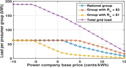
Fig. 5. Load of different groups in a single grid.
which the power company accounts for prosumer irrationality to the scenario in which the power company assumes that prosumers are rational. In both scenarios, the prosumers are irrational. For a reference point below $1, the company’s profits are barely affected. However, as the reference point crosses $1, the company’s profits start to show a clear decrease between the two scenarios. In fact, as the power company is not accounting for the prosumer’s actual subjec-tive behavior, its pricing strategy is no longer optimal. As was seen in Fig. 1, this is the reference point range where the total consumption mostly differs between CGT and PT. The decrease in profits reaches a peak value of 15 % at a reference point of $2. Clearly, the power company will experience a decrease in profits, if it neglects the subjective perception of prosumers.
Fig. 4 shows the total grid load energy consumption as function of the number of prosumers. The figure highlights the difference in consumption between rational prosumers and subjective prosumers with Rn = $1, which increases significantly with the number of prosumers in the grid. This difference reaches 100 kWh for 50 prosumers. This high-lights the impact of irrational behavior, which is prominent for larger grids.
Fig. 5 shows the energy consumption of different groups of prosumers, with different reference points, inside a single grid. For a very small ρbase, the different groups have equal consumption. As ρbase is increased to −5 cents, the prosumers withRn= $1start to decrease their consumption at equilibrium, while the other groups’ consumption remains unchanged. This is similar to what was discussed in Fig 1, where prosumers with reference points close to $1, exhibit
Number of prosumers
10 20 30 40 50 60 70
Iterations until convergence
10 15 20 25 30 35
Fig. 6. Number of iterations for convergence
risk averse behavior and thus lower energy consumption. On the other hand, rational prosumers will start decreasing their consumption at ρbase = 2 cents, while risk seeking prosumers (Rn= $3) will start decreasing their consumption atρbase= 5 cents.
Fig. 6 shows the number of iterations needed for the best response algorithm to converge to a followers’ NE for different number of prosumers, under PT. Clearly, the best response algorithm converges, for all these cases. In addition, the number of iterations needed for convergence is reasonable, even as the number of prosumers significantly increases from10to70.
VI. CONCLUSION
In this paper, we have proposed a novel framework for analyzing energy trading of prosumers with the power grid, while accounting for the uncertainty of the future price of energy. We have formulated the problem as a Stackelberg game between the power company (leader), seeking to maximize its profits by setting its optimal pricing strategy, and multiple prosumer (followers), attempting to choose the optimal amount of energy to trade. The prosumers game was shown to have a unique pure strategy Nash equilibrium under classical game theoretic analysis. Subsequently, we have used the novel concept of utility framing from prospect theory to model the subjective behavior of prosumers when faced with the uncertainty of future energy prices. Simulation results have highlighted the impact of behavioral considerations on the overall energy trading process.
As a future avenue of research, one can extend our model to a more dynamic multi-stage game that not only utilizes further capabilities of the storage devices (e.g. load shifting over time periods), but also admits efficient algorithms for obtaining its equilibrium points. In particular, devising in-centive compatible mechanisms for our model in the form of multi-stage dynamic game is an interesting future problem.
REFERENCES
[1] S.-C. Chan, K. M. Tsui, H. Wu, Y. Hou, Y.-C. Wu, and F. F. Wu, “Load-price forecasting and managing demand response for smart grids: Methodologies and challenges,”IEEE Signal Processing Magazine, vol. 29, no. 5, pp. 68–85, 2012.
[3] E. Bitar, R. Rajagopal, P. Khargonekar, and K. Poolla, “The role of co-located storage for wind power producers in conventional electricity markets,” inProceedings of the IEEE American Control Conference, San Francisco, CA, June 2011, pp. 3886–3891.
[4] C. Wu, H. Mohsenian-Rad, and J. Huang, “Wind power integration via aggregator-consumer coordination: A game theoretic approach,” in Proc. IEEE PES Innovative Smart Grid Technologies (ISGT), Washington, DC, USA, January 2012, pp. 1–6.
[5] Z. Chen, L. Wu, and Y. Fu, “Real-time price-based demand response management for residential appliances via stochastic optimization and robust optimization,”IEEE Transactions on Smart Grid, vol. 3, no. 4, pp. 1822–1831, 2012.
[6] N. Hajj and M. Awad, “A game theory approach to demand side management in smart grids,” inIntelligent Systems’. Springer, 2014, pp. 807–819.
[7] J. Chen, B. Yang, and X. Guan, “Optimal demand response scheduling with stackelberg game approach under load uncertainty for smart grid,” inIn proceedings of the IEEE Third International Conference on Smart Grid Communications (SmartGridComm), 2012, pp. 546–551. [8] M. Yu and S. H. Hong, “Supply–demand balancing for power
manage-ment in smart grid: A stackelberg game approach,”Applied Energy, vol. 164, pp. 702–710, 2016.
[9] S. Maharjan, Q. Zhu, Y. Zhang, S. Gjessing, and T. Bas¸ar, “Dependable demand response management in the smart grid: A stackelberg game approach,”IEEE Transactions on Smart Grid, vol. 4, no. 1, pp. 120– 132, 2013.
[10] F.-L. Meng and X.-J. Zeng, “An optimal real-time pricing for demand-side management: A stackelberg game and genetic algorithm ap-proach,” in2014 International Joint Conference on Neural Networks (IJCNN), 2014, pp. 1703–1710.
[11] W. Wei, F. Liu, and S. Mei, “Energy pricing and dispatch for smart grid retailers under demand response and market price uncertainty,”
IEEE transactions on smart grid, vol. 6, no. 3, pp. 1364–1374, 2015. [12] M. Zugno, J. M. Morales, P. Pinson, and H. Madsen, “A bilevel model for electricity retailers’ participation in a demand response market environment,”Energy Economics, vol. 36, pp. 182–197, 2013. [13] N. Liu, X. Yu, C. Wang, and J. Wang, “Energy sharing management
for microgrids with PV prosumers: A Stackelberg game approach,”
IEEE Transactions on Industrial Informatics, 2017.
[14] D. Kahneman and A. Tversky, “Prospect theory: An analysis of decision under risk,”Econometrica, vol. 47, no. 2, pp. 263–292, March 1979.
[15] A. Tversky and D. Kahneman, “Advances in prospect theory: Cumu-lative representation of uncertainty,”Journal of Risk and uncertainty, vol. 5, no. 4, pp. 297–323, October 1992.
[16] Y. Wang, W. Saad, N. B. Mandayam, and H. V. Poor, “Integrating energy storage into the smart grid: A prospect theoretic approach,” inProc. of IEEE International Conference on Acoustics, Speech and Signal Processing (ICASSP), Florence, Italy, May 2014, pp. 7779– 7783.
[17] W. Saad, A. L. Glass, N. B. Mandayam, and H. V. Poor, “Toward a consumer-centric grid: A behavioral perspective,” In Proceedings of the IEEE, vol. 104, no. 4, pp. 865–882, 2016.
[18] Y. Wang, W. Saad, N. B. Mandayam, and H. V. Poor, “Load shifting in the smart grid: To participate or not?”IEEE Transactions on Smart Grid, to appear, 2016.
[19] Y. Wang, W. Saad, A. I. Sarwat, and C. S. Hong, “Reactive power compensation game under prospect-theoretic framing effects,” IEEE Transactions on Smart Grid, 2017.
[20] L. Xiao, J. Liu, Y. Li, N. B. Mandayam, and H. V. Poor, “Prospect theoretic analysis of anti-jamming communications in cognitive radio networks,” inIn proc. of the IEEE Global Communications Conference (GLOBECOM), 2014, pp. 746–751.
[21] Y. Yang, L. T. Park, N. B. Mandayam, I. Seskar, A. L. Glass, and N. Sinha, “Prospect pricing in cognitive radio networks,”IEEE Transactions on Cognitive Communications and Networking, vol. 1, no. 1, pp. 56–70, 2015.
[22] R. Yang, C. Kiekintveld, F. Ord´o˜nEz, M. Tambe, and R. John, “Improving resource allocation strategies against human adversaries in security games: An extended study,”Artificial Intelligence, vol. 195, pp. 440–469, 2013.
[23] D. Kar, F. Fang, F. Delle Fave, N. Sintov, and M. Tambe, “A game of thrones: when human behavior models compete in repeated stackelberg security games,” inProceedings of the 2015 International Conference on Autonomous Agents and Multiagent Systems. International
Foun-dation for Autonomous Agents and Multiagent Systems, 2015, pp. 1381–1390.
[24] Q. Han, B. Dellaert, W. van Raaij, and H. Timmermans, “Inte-grating prospect theory and stackelberg games to model strategic dyad behavior of information providers and travelers: Theory and numerical simulations,” Transportation Research Record: Journal of the Transportation Research Board, no. 1926, pp. 181–188, 2005. [25] A.-H. Mohsenian-Rad, V. W. Wong, J. Jatskevich, and R. Schober,
“Optimal and autonomous incentive-based energy consumption scheduling algorithm for smart grid,” inInnovative Smart Grid Tech-nologies (ISGT), 2010. IEEE, 2010, pp. 1–6.
[26] C. Wang and M. De Groot, “Managing end-user preferences in the smart grid,” in Proceedings of the 1st International Conference on Energy-Efficient Computing and Networking. ACM, 2010, pp. 105– 114.
[27] Z. Han, D. Niyato, W. Saad, T. Bas¸ar, and A. Hjorungnes, Game Theory in Wireless and Communication Networks: Theory, Models, and Applications. Cambridge University Press, 2012.
[28] A. M. Finket al., “Equilibrium in a stochasticn-person game,” Jour-nal of Science of the Hiroshima University, Series ai (Mathematics), vol. 28, no. 1, pp. 89–93, 1964.
[29] L. S. Shapley, “Stochastic games,” Proceedings of the National Academy of Sciences, vol. 39, no. 10, pp. 1095–1100, 1953. [30] S. R. Etesami, W. Saad, N. Mandayam, and H. V. Poor, “Stochastic
games for smart grid energy management with prospect prosumers,”
arXiv preprint arXiv:1610.02067, 2016.
[31] J. B. Krawczyk and S. Uryasev, “Relaxation algorithms to find Nash equilibria with economic applications,”Environmental Modeling and Assessment, vol. 5, no. 1, pp. 63–73, 2000.
[32] F. Facchinei and C. Kanzow, “Generalized Nash equilibrium prob-lems,”4OR: A Quarterly Journal of Operations Research, vol. 5, no. 3, pp. 173–210, 2007.
[33] J. B. Rosen, “Existence and uniqueness of equilibrium points for concaven-person games,”Econometrica: Journal of the Econometric Society, pp. 520–534, 1965.
[34] D. Bertsekas, A. Nedi´c, and A. Ozdaglar, Convex Analysis and Optimization. Athena Scientific, 2003.
[35] R. T. Rockafellar and S. Uryasev, “Optimization of conditional value-at-risk,”Journal of risk, 2, pp. 21–42, 2000.
[36] L. P. Metzger and M. O. Rieger, “Equilibria in games with prospect theory preferences,” 2010.
[37] G. E. Rahi, A. Sanjab, W. Saad, N. B. Mandayam, and H. V. Poor, “Prospect theory for enhanced smart grid resilience using distributed energy storage,”arXiv preprint arXiv:1610.02103, 2016.
APPENDIXI PROOF OFTHEOREM1
First, we analyze the strictly concave expected utility of prosumer n in (7). By taking the second derivative of (7) with respect toxn, we get: ∂UnEUT
∂2x
n =−2α, which is a strictly
negative term, asα > 0. The optimal solution is either an interior point obtained by solving the necessary and sufficient optimality condition given by ∂U
EUT n
∂xn = 0, or is at one of
the boundaries, in case the interior solution is not feasible. Solving the optimality solution gives a unique solutionxr
n=
n maximizes each prosumer’s expected utility
function given that it lies in the feasible range ofXn.
APPENDIXII PROOF OFTHEOREM2
First, we show that the followers’ game is aconcave game
with closed and convex action sets in which the utility of player n is a concave function of its own action xn, for any fixed actions of others x−n. From (7), one can see
closed convex set. Using [33, Theorem 1], we can show that the prosumers’ game admits at least one pure strategy NE. For NE uniqueness, we use [33, Theorem 2] to show that the prosumers game is diagonally strictly concave. This means that one can find a fixed nonnegative vector r ≥ 0 such that for every two action profiles xo,x˜ ∈ X
We letIbe the identity matrix, andJ be a square matrix with all entries equal to 1. Then we can writeg(x,r) =Kx+c, whereK:=−α(I+J).Kis a negative definite matrix due to the positive definiteness ofI+Jand the fact that−α <0. By checking the diagonally strict concavity condition we get
(˜x−xo)′g(˜x,r) + (xo−x˜)′g(xo,r)
= (˜x−xo)′[Kxo+c] + (xo−x˜)′[Kx˜+c] =−(˜x−xo)′K(˜x−xo)>0, (14)
where the last inequality is due to the negative-definiteness of the matrix K. Using [33, Theorem 2] the NE will be unique.
APPENDIXIII
AUXILILIARY LEMMA FOR THE PROOF OFTHEOREM3
Lemma 1. There exists a constant K > 0 for which the
Nikaido-Isoda function Ψ(x,y) associated with the pro-sumers’ game satisfies Ψ(x,y) ≤ Kkx−yk. Moreover, Ψ(x,y)is convex inxand strongly concave inysuch that
Ψ(x, λy˜+ (1−λ)ˆy) =λΨ(x,y˜) + (1−λ)Ψ(x,yˆ)
+αλ(1−λ)kyˆ−˜yk2
, ∀λ∈[0,1]. (15)
Proof. For any two action profiles of the prosumers x = (x1, . . . , xn)∈ Ωand y = (y1, . . . , yn)∈Ω, the
Nikaido-Isoda function adopted for the utility in (7) will be:
Ψ(x,y) : = X
where the first inequality is due to the Cauchy-Schwarz inequality, andK :=p
n(θ+α(n+ 1)Bmax)2 is an upper
bound constant for the second term of the last equality. To
show the convexity ofΨ(x,y) with respect to x, let J be the n×n matrix with all entries equal to 1. Using (16), a simple calculation shows that ∇2
xxΨ(x,y) = 2αJ, where
∇2
xxΨ(x,y) denotes the Hessian matrix of Ψ(x,y) with
respect to variable vectorx. Sinceα >0andJ is a positive semi-definite matrix, this shows that ∇2
xxΨ(x,y) > 0,
which implies Ψ(x,y) is a convex function of x. Finally using (7), one can easily check that the equality in (15) holds, which shows that Ψ(x,y) is strongly concave with respect to its second argumenty.
APPENDIXIV PROOF OFTHEOREM3
We show that limt→∞x(t) = x∗, from Algorithm 1,
wherex∗ is a pure-strategy NE for the prosumers. To show that, we measure the distance of an action profilex(t)and its best response ΠΩa+Ax(t) using the Nikaido-Isoda
function and show that this distance decreases ast becomes large. In particular, we show that at the limit, this distance equals zero which shows that the limit point is an NE of the game.
Using the first part of Lemma 1, we have
Ψxr(t),xr(t+ 1)≤Kkxr(t)−xr(t+ 1)k
where the first equality is due to Lemma 1, and the last inequality is due to first part of Lemma 1 and the fact that xr(t) maximizes Ψ(x(t),·). Multiplying both sides of the
above inequality by α
2K2√t and defining c:=
α(n−1)D
4K and
at:= α
2K2√tΨ(x(t),x
r(t)), we get
at+1≤at−a2t+ c
t√t. (19)
Our goal is to show thatat<√2c×t−34 for allt≥ 100 c2,
in which case by definition ofatwe obtainΨ(x(t),xr(t)) = O(t−14). This not only shows thatlim
t→∞Ψ(x(t),xr(t)) =
0, implying that{x(t)} converges to a pure strategy NE of the prosumers game (note that Ψ(x,xr) = 0 if and only if
x is a NE), but it also shows that after t steps, the action profile of the prosumersx(t)is anǫ-NE of the game where
ǫ = O(t−14) (this is due to Ψ(x(t),xr(t)) = O(t− 1 4)
im-plies Un(xr
n(t),x−n(t), ρbase)−Un(xn(t),x−n(t), ρbase) =
O(t−1
4) for all n ∈ N, meaning that given the action
profile x(t), no prosumer can increase its utility by more thatO(t−1
4)by playing its best response).
We complete the proof using induction ontto show that
at<√2c×t−3
4. Assume that this relation is true fort. Then
at+1≤at−a2t + c t√t ≤√2ct−34−2ct−
3 2+ c
t√t =√2ct−34−ct−
3 2.
Let f(z) : [1,∞) → R be a function defined by f(z) = √
2cz−3
4 −√2c(z+ 1)− 3 4 −cz−
3
2. We only need to show
thatf(z)<0,fort≥100
c2 . By writing the Taylor expansion
of the first two terms of f(z) forz ≥1, we have f(z)≤ 7√2cz−7
4 −cz− 3
2, which is less than 0 for t ≥ 100 c2 . This
completes the induction and shows that at=O(t−34).
APPENDIXV PROOF OFTHEOREM4
We first find the conditions under which the expected utility function is uniform over each prosumer’s action space. We then find the additional condition to ensure that the function is strictly concave.
Case 1:To haveRn< ρminc+d, for all of prosumern’s actions, we first rewrite the inequality in terms ofxn:
−αx2n+ (ρmin−ρb−αx¯−n)xn+ (ρminKn−Rn)<0, wherekn =Wn+Qn−Ln. By analyzing the second order polynomial, and its roots,r1andr2, we get the condition for
case1. Under such a condition, the expected utility function of prosumernunder PT, simplifies toUPT
n (xn,x¯−n, ρbase) =
UEUT
n (xn,x¯−n, ρbase)−Rn. This is clearly a concave func-tion, given that,UEUT
n (xn,x¯−n, ρbase)has been shown to be concave, andRn is a constant.
Case 2: In order to have Rn > ρmaxc +d, for all
of prosumer n’s actions, we follow a similar approach in order to find the condition for case 2. Under this con-dition, the expected utility function under PT simplifies
to UPT
n (xn,x¯−n, ρbase) = λ(UnEUT(xn,x¯−n, ρbase)−Rn),
which is also strictly concave, given thatλis strictly positive.
Case 3: To have ρminc+d < Rn < ρmaxc+d, for all of prosumer n’s actions, we follow a similar approach in order to find the condition for case 3. We next analyze the concavity of the expected utility function, given in the second line in (12). The second derivative is given by:
∂Un,P T ∂2x
n = a1
m1x
n−a1m1−bm1 m2
1
− (λ−1)a
2 2
(Qn−Ln+Wn+xn)3,
where a2 = (Rn −(knρbase) +α(L2n +Q2n +w2n)−
2LnQnα+Lnαx¯−n−Qnαx¯−n−2Lnαwn+2Qnαwn. Note
that− (λ−1)a
2 2
(Qn−Ln+Wn+xn)3 is negative for allxn. Next, we find
the range ofxn for which a1 m1xn−
a1m1−b1m1 m2
1
is negative as well. Given that a1
m1 is negative, the utility function is thus