arXiv:1711.06641v1 [cs.GT] 17 Nov 2017
The Complexity of Multiwinner Voting Rules with Variable
Number of Winners
Piotr Faliszewski
AGH University
Krakow, Poland
Arkadii Slinko
University of Auckland
Auckland, New Zealand
Nimrod Talmon
Weizmann Institute of Science
Rehovot, Israel
November 20, 2017
Abstract
We consider the approval-based model of elections, and undertake a computational study of voting rules which select committees whose size is not predetermined. While voting rules that output committees with a predetermined number of winning candidates are quite well studied, the study of elections with variable number of winners has only recently been initiated by Kilgour [18]. This paper aims at achieving a better understanding of these rules, their computational complexity, and on scenarios for which they might be applicable.
1
Introduction
We study the setting where a group of agents (the voters) want to select a set of candidates (a committee) based on these agents’ preferences. Agents are asked which candidates they approve of for the inclusion into the committee and this input data needs to be aggregated. However, as opposed to the quickly growing body of work on electing committees of a fixed size [14, 15, 3, 1, 17], here we are interested in rules that derive both the size of the winning committee and its members from the voters’ preferences. Recently, Kilgour [18] and Duddy et al. [13] initiated a systematic study of such voting rules; here we are interested in the complexity of computing their winners and in experimentally analyzing the sizes of the elected committees (for some early axiomatic results, we also point the reader to the work of Brandl and Peters [9]).
1.1
When Not To Fix the Size of the Committee?
There is a number of settings where it is not natural to fix the size of the committee to be elected and it is better to deduce it from the votes. Since so far committee elections with variable number of winners did not receive much attention in the AI literature, below we provide a number of examples of such settings. We do not mention this repeatedly, but one may wish to automate the processes in the examples below using AI techniques.
but we have a number of easy to evaluate (but imperfect) criteria that the selected items should satisfy (these criteria are soft and it may be that the best item actually fails some of them). We view each criterion as a voter (who “approves” the items that satisfy it) and we seek a committee, hopefully of a small size, of candidates from which the qualified expert will choose the final item.1
Initial screening is closely related to shortlisting [4, 14]. We use a different name for it to emphasize that we do not fix the number of candidates to choose, as is the case with shortlisting.
Finding a Set of Qualifying Candidates. Finding a set of candidates that satisfy all or almost all criteria is a common problem. Real-life examples include selecting baseball players for inclusion into the Hall of Fame and selecting students to receive an honors degree. In the former case, eligible voters (baseball writers) approve up to ten players and those approved by at least 75% of the voters are chosen to the Hall of Fame. In the latter case, the voting process is typically implicit; the university announces a set of criteria of excellency—which act as voters, “approving” the students that satisfy them2—and set rules such as “a student receives an honors degree if he or she meets at
least five out of six criteria”. It is often desirable that the selected committee is small (say, at most a few people for the Hall of Fame and some not-too-large percentage of the students for the honors degree), but this is not always the case. E.g, consider the task of selecting people for an in-depth medical check based on a number of simple criteria that jointly indicate elevated risk of a certain disease; everyone who is at risk should be checked regardless of the number of those patients.
One of the first procedures formally proposed for the task of selecting a group of qualifying candidates was the majority rule (MV), suggested by Brams, Kilgour, and Sanver [8]. The majority rule outputs the committee that includes all the candidates that are approved by at least half of the voters (satisfy at least half of the criteria). It is, of course, natural to consider MV with other thresholds, as, for example, in the Hall of Fame example.
Partitioning into Homogeneous Groups. For the case of partitioning candidates into homoge-neous groups, we can no longer focus only on one of the groups (the committee), but rather we care about a partition into two groups so that each of them contains candidates that are as similar as possible. A prime example here is partitioning students in some class into two groups, e.g., a group of beginners and a group of advanced ones (say, regarding, their knowledge of a foreign language; depending on the setting, it may or may not be important to keep the sizes of these two groups close). The students are partitioned in this way to facilitate a better learning environment for everyone; in the context of voting, the issue of partitioning students was raised by Duddy et al. [13].
Finding a Representative Committee. An elected committee is representative if each voter approves at least one committee member (who then can represent this voter). The idea of choosing a representative committee of a fixed size received significant attention in the literature (see the works of Chamberlin and Courant [10], Monroe [21], Elkind et al. [14], and Aziz et al. [2] as some examples). However, as pointed out by Brams and Kilgour [7], committees of fixed size simply cannot always provide adequate representation. Thus, in some applications, it is natural to elect committees without prespecified sizes (while in others, fixing the committee size may be necessary). A representative committee may be desired when some authorities are revising existing regu-lations and need to consult citizens, for which purpose they would like to select a representative focus groups in various cities. The people in a focus group do not have to represent the society proportionally (their role is to voice opinions and concerns and not to make final decisions), but
1
One of the authors of this paper was once tasked with the problem of classifying a collection of daggers for a museum. The solution was to compute a number of partitions of the set of daggers into clusters, evaluate their qualities without reference to ethnographical knowledge on the daggers, and to present the best ones to the museum’s experts, who chose one partition that led to an ethnographically meaningful classification.
2
should cover all the spectrum of opinions in the society. Usually, small representative committees are more desirable than larger ones.
1.2
Our Contribution
Our main goal is to study computational aspects of voting rules tailored for elections with a variable number of winners. This direction was pioneered by Fishburn and Pekeˇc [16], who introduced the class of threshold rules and studied their computational complexity (somewhat surprisingly, only for the case when the committee size is fixed). We are not aware of other computational studies that followed their work.
In this paper we study the threshold rules of Fishburn and Pekeˇc [16], as well as a number of other rules, including those discussed by Kilgour [18]. We obtain the following results:
1. For each of the rules, we establish whether finding a winning committee under this rule is in P or is NP-hard (in which case we seek FPT algorithms parameterized by the numbers of candidates and by the number of voters).
2. We evaluate experimentally the average sizes of committees elected by our rules. We consider a basic model of preferences, where each voter approves each candidate independently, with some probabilityp(we focus onp=1/2but for some representative rules we consider a larger
spectrum of probability values).
We only make preliminary comments regarding suitability of our rules for the tasks outlined above. While specifying the applications is important to facilitate future research, we believe that we are still at the level of identifying voting rules and gathering basic knowledge about them.
2
Preliminaries
An approval-based election E = (C, V) consists of a set C = {c1, . . . , cm} of candidates and a collectionV = (v1, . . . , vn) of voters. Voters express their preferences by filling approval ballots. The
approval ballot of a voter specifies the subset of candidates that this voter approves. To simplify notation, we denote votervi’s approval ballot also asvi (whether we mean the voter or the subset of approved candidates will always be clear from the context). A collectionV of voters, interpreted as a collection of approval ballots in a certain election, is called the preference profile. For a given subsetS of the candidates from setC, byS we mean the candidates not inS, i.e.,S=C\S. By theapproval scoreof a candidate in an election, we mean the number of voters that approve of this candidate.
A voting rule for elections with a variable number of winners is a function R that, given an electionE = (C, V), returns a family of subsets of C (the set of committees which tie as winners). The main point of difference between the type of voting rules that we study here and the voting rules typically studied in the context of multiwinner elections is that we do not fix the size of the committee to be elected and we let it be deduced by the rule.
For an overview of multiwinner election procedures using approval balloting, we point to the works of Kilgour [17, 18], both for the discussions of rules with fixed and variable number of winners; Duddy et al. [9] and Brandl and Peters [13] discuss the polynomial-time computable Borda mean rule (not included in our discussion).
Our hardness results follow by reductions from the NP-complete problem Set Cover. An
instance of Set Coverconsists of a set U ={u1, . . . , un} of elements, a familyS ={S1, . . . , Sm}
3
Simple Approval Rule
We start our discussion by considering the Approval rule (AV), one of the arguably simple rules for the setting with variable number of winners.
Approval Voting (AV). Under AV we output the (unique) committee of candidates with the highest approval score.
In essence, AV is the single-winner Approval rule which instead of breaking ties (among winning candidates) outputs all the candidates with the highest score. The rule is, of course, polynomial-time computable.
Proposition 1. There is a polynomial-time algorithm that computes the unique winning committee under the AV rule.
We should expect the winning committees for this rule to be very small and, indeed, the following experiment confirms this intuition (the AV rule is so simple that the experiment is not really neces-sary; we include it for the sake of completeness and to provide the setup for experiments regarding less intuitive rules).
Experiment 1. We consider elections with m= 20 candidates andn= 20 voters, where for each candidate c, each voter approves c with probability p = 1/2. We have generated 10,000 elections
and the average committee size was 1.52 with standard deviation 0.89. (See Table 1 for the list of average committee sizes in this setting for our rules; to see how the number of voters affects the average committee sizes, we also included experiments for 20candidates and100voters). We repeat this experiment for all the rules in this paper.
Remark 1. We have chosen a fairly small number of candidates and voters for our experiments as the results for such elections are fast to compute (even for NP-hard voting rules) and, yet, they appear to be sufficient to show the effects that we are interested in. We chose the model where each candidate is approved or disapproved independently by each voter because it is the most basic scenario which, we believe, one should start with (other scenarios should be considered in future works).
4
(Generalized) Net-Approval Voting
In the framework where the size of the target committee is fixed, one may ask for a committee of candidates whose sum of approval scores is the highest. To adapt this idea to the variable number of winners, Brams and Kilgour [7] suggested the Net-Approval Voting (NAV) rule. This rule pays attention not only to approvals but also to disapprovals.
Net Approval Voting (NAV). The score of a committeeS in electionE= (C, V) under NAV is defined to beP
vi∈V |S∩vi|−|S∩vi|
; the committees with the highest score tie as co-winners.
Note that this rule is very close to the MV rule [8] mentioned in the introduction; the winning committees under NAV consist of all candidates approved by a strict majority of the voters and any subset of those approved by exactly half of the voters (MV includes all candidates approved by at least half of the voters).
Corollary 2. There is a polynomial-time algorithm that computes the unique smallest3 winning
committee under the NAV rule.
3
Experiment 2. Repeating Experiment 1 for NAV, we obtain 8.25 as the average size of the small-est elected committee with standard deviation 2.19. This confirms the intuition that slightly fewer than half of the candidates would be elected in a typical election, where each candidate is approved independently with probability 1/2 (since in the smallest winning committee it is necessary to be
approved by more than half of the voters). We also computed the average size of a NAV com-mittee for the case where voters approve candidates with other probabilities. Specifically, for each
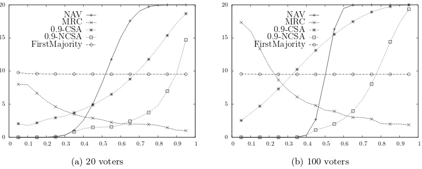
p∈ {0.05,0.1, . . . ,0.95}we generated10,000elections with20candidates and20voters, where each voter approves each candidate with probabilityp, and we computed the average size of the NAV com-mittee. We repeated the same experiment for20candidates and100voters. The results are presented in Figure 2. We see that when the number of voters becomes large, the graph becomes very close to the step function. This means that NAV should only be used in very specific settings (such as the baseball Hall of Fame example).
It turns out that, using the main idea behind the NAV rule, it is possible to express many different voting rules. Below we suggest a language for describing such rules.
Generalized NAV. Letf andg be two non-decreasing, non-negative-valued functions,f, g:N→
N, such that f(0) = g(0) = 0. We define the (f, g)-NAV score of a committee S in election
E= (C, V) to be:
P
vi∈V f(|S∩vi|)−g(|S∩vi|)
.
The committees with the highest score tie as co-winners. The intuition for this rule is that we would like to be able to count approvals and disapprovals differently. E.g., this can be explained as follows: at times, the lack of approval of a candidate is not really a disapproval but lack of information about him/her or simply no firm opinion.
Remark 2. It would also be reasonable to include the terms f′(|S∩v
i|)and−g′(|S∩vi|)(for two
additional functions f′ and g′) in the definition of the score above. The first term, for example,
would reflect the utility that votervi has from exclusion of candidates whom he/she did not approve. (f, g)-NAV rules are quite diverse. For example, iff and g are linear functions (e.g., f(x) = x and g(x) = 2x) then (f, g)-NAV is a variant of the MV rule with a different threshold of approval (for the given example, a candidate would be included in the committee if it were approved by at least a 2/3 fraction of the voters; thus, we refer to this rule also as 2/3-NAV). Such rules seem
quite appropriate for the task of choosing a set of qualifying candidates as, for each candidate c, the decision whether to include c in the committee or not is made based on approvals for c only (indeed, the decision if a patient should be sent for an in-depth medical check should not depend on the health of other patients).4 Below we show that for nonlinear functionsf and g, (f, g)-NAV
rules might no longer have this independence property.
Let us consider the functiont1(x), wheret1(0) = 0 andt1(k) = 1 for eachk≥1. Then, the rule
(t1,0)-NAV, where we write 0 to mean the function that takes value 0 for all its inputs, seeks
com-mittees where each voter approves at least one committee member. In consequence, the committee that consists of all candidates is always winning under this rule (and, of course, also polynomial-time computable). However, it is far more interesting to seek the smallest (t1,0)-NAV winning committee
and we refer to the rule that outputs such committees as the Minimum Representation Rule (MRC). A more intuitive description of this rule follows.
Minimal Representing Committee rule (MRC). Under the MRC rule, we output all the com-mittees of smallest size such that each voter (with a nonempty approval ballot) approves at least one of the committee members.
4
Intuitively, MRC is very close to the approval variant of the Chamberlin–Courant rule [10, 23, 5]; we refer to the approval-based Chamberlin–Courant rule as CC. Under CC, we are given an approval election E = (C, V), a committee size k, and our goal is to find a committee of sizek such that as many voters as possible approve at least one of the committee members (for the case of CC, typically the fact that a voter approves a candidate is interpreted as saying that the voter would feel represented by this candidate). MRC is, in a sense, a variant of CC where we insist that each voter be represented, but we want to keep the committee as small as possible.
Since computing an MRC winning committee means, in essence, solving the minimization version of the Set Cover problem, we next proposition follows (missing hardness proofs are available in
the supplementary material).
Proposition 3. Given an electionE and a positive integerk, it isNP-hard to decide if there is an MRC winning committee of size at mostk.
Proof. It suffices to note that our problem is equivalent to theSet Cover problem. To see this,
consider a Set Cover instance with I = (U,S, k), where U ={u1, . . . , un} is a set of elements,
S ={S1, . . . , Sm} is a family of subsets ofU, andk is an integer. We form an electionE = (C, V) where for each setSi we have a candidatesi and for each elementuj we have a voter that approves exactly those candidates si for whichuj ∈Si. There is a winning MRC committee of size at most kif and only if there is a collection of at most ksets that coverU.
Fortunately, computing MRC winning committees is fixed-parameter tractable (is in FPT) when parameterized by either the number of candidates or the number of voters (we omit the proof due to space restriction, but mention that the ideas are similar to those that we use for Theorem 9).
Proposition 4. The problem of deciding if there is an MRC winning committee of size at most k
(in a given election E) is in FPT, when parameterized either by the number of candidates or the number of voters.
Proof. The result for the number of candidates follows via a straightforward brute-force algorithm. For parameterization by the number of voters, we invoke the “candidate types” idea of Chen et al. [11]: There are at most 2n “candidate types” (where the type of a candidate is simply the set of voters that approve of him or her). Then, we observe that it suffices to consider at most one candidate of each type, since a winning committee certainly never contains two candidates of the same type because we could remove one). In FPT-time, we try all possible committees of at most 2n candidates (of different types).
Experiment 3. By applying Experiment 1 to MRC, we obtain that the average committee size is
2.68with standard deviation0.46. Since the rule isNP-hard, we have used the brute-force algorithm to try all possible committees. We also present results for other probabilities of approving each candidate (see Figure 2). A positive feature of this rule is that the size of a winning committee does not depend much on the number of voters.
We can also use the standard greedy algorithm forSet Coverto find approximate MRC
com-mittees; indeed, we view this algorithm as a voting rule in its own right.
Experiment 4. By connection to Set Cover, GreedyMRC is guaranteed to find a committee that is at most a factorO(logm)larger than the one given by the exact MRC (where mis the number of candidates). In our experiment, with approval probabilities in {0.05,0.1, . . . ,0.95}, the average sizes of the GreedyMRC committees where no more than 8% larger than the average sizes of the MRC ones (for the case of 20 voters) or no more than 11% larger (for the case of 100 voters).
MRC and GreedyMRC appear to be well suited for choosing small committees of representative; our experiments confirm this intuition.
Recall that the functiont1(x) is such thatt1(0) = 0 andt1(k) = 1 for eachk≥1. Then, consider
the (0, t1)-NAV rule, which elects all the committees that contain candidates approved by all the
voters. While the empty set is trivially a winning committee under this rule, it is more interesting to ask about the largest winning committee; we refer to the rule that outputs the largest winning (0, t1)-NAV rule as the unanimity rule:
Unanimity Voting (UV). Under the unanimity rule, we output the committee of all the candi-dates approved by all the voters.
While computing the smallest (t1,0)-NAV winning committee is hard (Proposition 4), it is easy
to compute the (unique) largest (0, t1)-NAV winning committee in polynomial time (i.e., there is a
polynomial-time algorithm for UV).
Experiment 5. As expected, in our experiment it never happened that some candidate was approved by all the voters (the probability of some candidate being approved by all 20 voters is 20·2−20 and
we considered only 10,000 elections).
Both for (t1,0)-NAV and for (0, t1)-NAV, it is trivial to computesome winning committee (the
set of all candidates in the former case and the empty set in the latter). In general, however, this is not the case.
Theorem 5. There exists an (f, g)-NAV rule for which deciding if there exists a committee with at least a given score isNP-hard.
Proof. We consider specific functionsf andgand show that for the corresponding (f, g)-NAV rule it is NP-hard to decide if there exists a committee with at least a given score. The specific functions f andg we consider are as follows:
f(x) = (
0, x= 0
4, x≥1 g(x) =
0, x= 0 1, x= 1 2, x≥2
To show NP-hardness, we reduce from the NP-hard X3C problem. In it, we are given sets
S={S1, . . . , Sn}over elementsb1, . . . , bn. Each set contains exactly three integers and each elements
is contained in exactly three sets. The task is to decide whether there is a set of setsS′ ⊆ S such
that each elementbi is covered exactly once. We assume, without loss of generality, thatn >39. Given an instance of X3Cwe create an election as follows. For each setSjwe create a candidate
Sj. For each element bi we create three voters: vi1 vi2, and v3i; v1i and vi2 are referred to as set
voters whilev3
i is referred to asantiset voter. Both votersvi1andvi2approve exactly the candidates corresponding to the sets which contain bi, while the voter v3
whether a committee with score at least 7n exists. This finishes the description of the reduction. Next we prove its correctness.
LetC be a committee for the reduced election and letbi be some element of theX3C instance. First we show thatC has at least six candidates in it. If it is not the case, then, since each set Sj covers exactly three elements, it follows that there are at leastn−18 elements not covered byC.
Letbi be an element not covered by C. Then, the votersv1i,vi2, andv3i corresponding tobigive at most 2 points toC. IfC=∅then each voter corresponding tobi gives 0 points toC. Otherwise, ifC6=∅, then each set voter (each ofvi1orvi2) gives at most−1 points toC, while the antiset voter gives at most 4 points. Thus, the voters corresponding tobi give at most 2 points to C.
There are at most 18 elements which are covered by C. For each bi which is covered byC, each of the votersv1
i,v2i, andv3i corresponding tobigive at most 4 points tobi(since this is the maximum number of points any voter gives to any committee). Thus, the voters corresponding tobi give at most 12 points toC.
Summarizing the above two paragraphs, we have that the total score ofCwhich has at most six candidates is at most (3k−18)·2 + 18·12. Since we assume, without loss of generality, thatn >39, we have that this quantity is strictly less than 7n. Therefore, from now on we assume thatChas at least six candidates in it.
Thus, let C be a committee with at least six candidates in it and let bi be an element. Let Vi = {vi1, vi2, v3i} and consider the following four cases depending on the number of times bi is covered by the setsSj corresponding to the candidates inC.
• bi is not covered byC: In this case, the score given toCbyViis at most (−2)+(−2)+4 = 0.
To see this, observe that each of the set voters (v1
i, v2i) gives toCexactly−2 points, since they do not approve any candidate fromCbut disapprove all candidates inC; further, observe that the antiset voter (v3
i) gives toC at most 4 points, as this is the maximum number of points any voter can give to any committee.
• bi is covered exactly once byC: In this case, the score given toCbyViis 2 + 2 + 4−1 = 7.
To see this, observe that each of the set voters (v1
i, vi2) gives toC exactly 2 points, since they approve one candidate from C (the one candidate corresponding to the one set coveringbi) and disapprove all other candidates in C; further, observe that the antiset voter (v3
i) gives to C exactly 3 points, since it approves at least one candidate inC and disapprove exactly one candidate in C (the one candidate corresponding to the one set coveringbi).
• biis covered more than once byC: In this case, the score given toCbyViis 2+2+4−2 = 6.
To see this, observe that each of the set voters (v1
i, vi2) gives toC exactly 2 points, since they approve more than one candidate from C (the two or three candidates corresponding to the two or three sets covering bi) and disapprove all other candidates in C; further, observe that the antiset voter (vi3) gives toC exactly 2 points, since it approves at least one candidate in C and disapprove two or three candidates inC(the two or three candidates corresponding to the two or three sets coveringbi).
As there are exactlynelements, it follows from the case analysis above that a committeeCwith score at least 7nshall correspond to an exact cover.
5
(Net-)Capped Satisfaction and FirstMajority
Kilgour and Marshall [19] introduced the following rule in the context of electing committees of fixed size, and Kilgour [18] recalled it in the context of elections with a variable number of winners, suggesting its net version.
Capped Satisfaction Approval (CSA). The Capped Satisfaction Approval (CSA) score of a committee S is defined to be P
vi∈V
|S∩vi|
|S| . The committees with the highest score tie as
co-winners.
Net Capped Satisfaction Approval (NCSA). The NCSA rule uses the “net” variant of CSA score; specifically, the score of a committee S is defined to be P
vi∈V
|S∩vi|
|S| − |S∩vi|
|S| and the
committees with the highest score tie as co-winners.
In the definitions above, the idea behind dividing the scores by the size of the committee is to ensure that committees which are too large will not be elected. Unfortunately, for the rules as defined by Kilgour [18], this effect is too strong, leading mostly to committees containing only the candidate(s) with the highest approval score. We explain why this is the case and suggest a modification.
Consider an election E = (C, V) with candidate set C = {c1, . . . , cm} and preference profile V = (v1, . . . , vn). Let s(c1), . . . ,s(cm) be the approval scores of the candidates, and, without loss
of generality, assume that s(c1) ≥ s(c2) ≥ . . . ≥ s(cm). Note that, if there are no ties regarding
the approval scores, then for each k, the highest-scoring CSA committee of size k is simplySk =
{c1, . . . , ck}and its score isPvi∈V never increases with k and, so, typically CSA outputs very small committees (which contain only the candidates with the highest approval score; the same reasoning applies to NCSA). Thus, we introduce the q-CSA and the q-NCSA rules, where q is a real number, 0 ≤ q ≤ 1, and (a) the
NCSA, whereas 0-NCSA is NAV and 0-CSA is a rule that outputs the committee that includes all the candidates that receive any approvals.
By the reasoning above, for each rational value ofq, bothq-CSA andq-NCSA are polynomial-time computable (using notation from previous paragraph, it suffices to consider the committees S1, S2, . . . , Smand output the one with the highestq-CSA orq-NCSA score, respectively).
Proposition 6. For each rational value of q, there is a polynomial-time algorithm that, given an election, computes a winning committee for q-CSA and for q-NCSA.
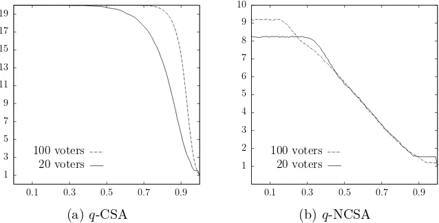
Experiment 6. To obtain some better understanding of the influence of the parameterqon the size of the committees elected according to q-CSA and q-NCSA, we have repeated Experiment 1 (with approval probabilityp=1/2) for these rules for qvalues between0and1 with step0.01. The sizes of
the average committee that we obtained are presented in Figure 1. The figures show results for the case of20candidates and either20or100voters. While the average committee size forq-NCSA does not depend very strongly on the number of voters (and its dependence onq is appealing), the results for q-CSA are worrying. Not only does the rule elect (nearly) all candidates for most values of q, but also for the values where it is more selective (e.g., q= 0.9), the average size of its committees depends very strongly on the number of voters. In Figure 2 we show average sizes of0.9-CSA and of
1
Figure 1: Average committee sizes (y-axis) underq-CSA andq-NCSA rules for different values ofq (x-axis); see Experiment 1 for information on how the elections were generated.
worries regardingq-CSA rules. While the dependence of the average committee size on the candidate approval probability for 0.9-NCSA has the same nature irrespective of the number of voters (it is, roughly speaking, convex both for20 and100voters), the same dependence for0.9-CSA changes its nature (from roughly convex for the case of20voters to roughly concave for the case of100voters). In Table 1 we also show average committee sizes for0.5-CSA and0.5-NCSA for the candidate approval probability p=1/2.
Given the above experiments, we believe that for practical applications, where we may have limited control on the number of candidates, the number of voters, and the types of the votes cast, choosing an appropriate value of the parameterqforq-CSA rules (e.g., to promote committees close to a particular size) would be very difficult. On the other hand, q-NCSA might be robust enough as to be practical.
One could consider generalized variants of the q-CSA andq-NCSA rules in the same way as we have considered generalized NAV rules. We leave this as future work and we conclude the section by considering a different rule of Kilgour [18], which is not an (N)CSA rule, but which is somewhat similar since it also chooses a certain number of candidates with the highest approval scores.
FirstMajority. Consider an election with candidatesC ={c1, . . . , cm}. For each ci ∈ C denote of voters then this rule may return more than one committee, corresponding to the various possible ways of reordering the candidates.
The very definition of FirstMajority gives a polynomial-time algorithm for computing its winning committees.
Experiment 7. Under our experimental setup (see Experiment 1), on the average, the FirstMajority rule outputs committees of size9.51(with standard deviation0.43). Further, the size of the committee is almost independent of the number of voters and the candidate approval probability (see Figure 2).
6
Threshold Rules
We conclude our discussion by considering the threshold rules of Fishburn and Pekeˇc [16]. Let t:N→Nbe some function referred to as thethreshold function. Thet-Threshold rule is defined as
follows.
t-Threshold. Consider an electionE = (C, V). Under the t-Threshold rule, we say that a voter
vi ∈ V approves a committee S if |S ∩vi| ≥ t(|S|). The t-Threshold rule outputs those committees that are approved by the largest number of voters.
We consider the following three (in some sense extreme) examples of threshold functions: (a) the unit function tunit = t1 (recall the discussion of generalized net-approval rules); (b) the majority
function,tmaj(k) =k/2; and (c) the full function,tfull(k) =k.
Thetunit-Threshold rule is very similar to MRC because, under the tunit threshold function, a
voter approves a committee if it includes at least one candidate that this voter approves. Thus the rule outputs all committeesS such that each voter with a nonempty approval ballot approves some member of S (MRC outputs the smallest of these committees). Thus finding the largest winning committee is easy (take all the candidates), but finding the smallest one is hard (as then we have the MRC rule).
On the other hand, the tfull-Threshold rule outputs exactly those committees S that (a) each
candidate inS has the highest approval score and (b) all the candidates inS are approved by the same group of voters. It seems, however, that AV is a simpler and more natural rule than the tfull-Threshold rule.
Finally, we consider thetmaj-Threshold rule, introduced and studied by Fishburn and Pekeˇc [16];
tmaj-Threshold winning committees receive broad support from the voters, and—as suggested by
Fishburn and Pekeˇc—should be “of moderate size”. Computingtmaj-Threshold winning committees
is NP-hard, but there are FPT algorithms.
Theorem 8. The problem of deciding if there is a nonempty committee that satisfies all the voters under thetmaj-threshold rule isNP-hard.
Proof. We give a reduction from theSet Coverproblem. Let our input instance be I= (U,S, k),
whereU ={u1, . . . , un} is a set of elements,S ={S1, . . . , Sm} is a family of subsets ofU, and kis a positive integer. Without loss of generality, we can assume thatm > k(otherwise there would be a trivial solution for our input instance).
We form an election with the candidate setC=F∪ S, whereF ={f1, . . . , fk} is a set of filler candidates andS is a set of candidates corresponding to the sets from theSet Coverinstance (by
a small abuse of notation, we use the same symbols forSand its contents irrespective if we interpret it as part of theSet Coverinstance or as candidates in our elections). We introducekn+ 2 voters:
1. The first voter approves of all the filler candidates and the second voter approves all the set candidates. We refer to these voters as the balancing voters.
We claim that there is a nonempty committee S such that every voter approves at least half of the members ofS (i.e., every voter is satisfied) if and only if Iis ayes-instance.
Let us assume thatSis a committee that satisfies all the voters. We note thatSmust contain the same number of filler and set candidates. If it contained more set candidates than filler candidates then the first balancing voter would not be satisfied, and if it contained more filler candidates than set candidates, then the second balancing voter would not be satisfied. Thus, there is a number k′
such that|S|= 2k′,k′≤k, andS contains exactlyk′ filler andk′ set candidates.
We claim that these k′ set candidates correspond to a cover of U. Consider some arbitrary element ui and some filler candidatefj such thatfj does not belong to S (since m > k≥k′ such candidates must exist). There is a voter that approves all the filler candidates exceptfj and all the set candidates that containui. Thus, the committee contains exactlyk′−1 filler candidates that
this voter approves and—to satisfy this voter—must contain at least one set candidate that contains ui. Since ui was chosen arbitrarily, we conclude that the set candidates fromS form a cover of U. There are at mostkof them, soI is ayes-instance.
On the other hand, if there is a family ofk′≤ksets that jointly coverU, then a committee that
consists of arbitrarily chosenk′ filler candidates and the set candidates corresponding to the cover
satisfies all the voters.
Theorem 9. Let t be a linear function (i.e., t(k) = αk for some α ∈ [0,1]). There are FPT
algorithms for computing the smallest and the largest winning committees under the t-Threshold rule in FPTtime for parameterizations by the number of candidates and by the number of voters. Proof. For parameterization by the number of candidates it suffices to try all possible committees. For parameterization by the number of voters, we combine the candidate-type technique of Chen et al. [11] and an integer linear programming (ILP) approach. Thetype of candidatecis the subset of voters that approvec. For an election withn voters, each candidate has one of at most 2n types. We describe an algorithm for computing a committee approved by at least N voters (where N is part of the input; it suffices to try all values ofN ∈[n] to find a committee with the highest score). We focus on computing the largest winning committee.
LetE= (C, V) be the input election withnvoters. We form an instance of the ILP problem as follows. For each candidate typei, i∈ [2n], we introduce integer variablex
i (intuitively xi is the number of candidates of type ithat are included in the winning committee). For eachi∈[2n], we form constraint 0≤xi ≤ni, whereni is the number of candidates of typeiin electionE. We also add constraintP
i∈[2n]xi≥1 as the winning committee must be nonempty.
For each voterj ∈[n], we define an integer variable vj (the intention is that vj is 1 if the jth voter approves of the committee specified by variablesx0, . . . , x2n−1 and it is 0 otherwise; see also
comments below). For eachj∈[n], we introduce constraints 0≤vj≤1, and:
P
i∈types(vj)xi
−tP i∈[2n]xi
≥ −(1−vj)n, (1)
where types(vj) is the set of all candidate types approved by voter vj. To understand these con-straints, note thatP
i∈[2n]xi is the size of the selected committee,Pi∈types(vj)xi is the number of
0 5 10 15 20
0 0.1 0.2 0.3 0.4 0.5 0.6 0.7 0.8 0.9 1
NAV MRC 0.9-CSA
0.9-NCSA
FirstMajority
(a) 20 voters
0 5 10 15 20
0 0.1 0.2 0.3 0.4 0.5 0.6 0.7 0.8 0.9 1
NAV MRC 0.9-CSA
0.9-NCSA
FirstMajority
(b) 100 voters
Figure 2: Average committee sizes for some of our rules (20 candidates and either 20 or 100 voters; approval probability is on the x-axis).
rule avg. committee size± complexity
its std. deviation
(20 voters) (100 voters)
2/3-NAV 1.02±1.01 0.01±0.09 P
AV 1.52±0.89 1.20±0.50 P
0.9-NCSA 1.52±0.89 1.50±0.78 P
MRC 2.63±0.48 4.08±0.26 NP-hard
GreedyMRC 2.75±0.46 4.55±0.53 P tmaj-Thr (min) 2.75±1.33 2.05±0.34 NP-hard
0.5-NCSA 5.57±2.14 5.57±2.18 P 0.9-CSA 5.63±3.02 14.67±2.75 P
tmaj-Thr (max) 7.68±3.27 2.20±0.78 NP-hard
NAV 8.25±2.19 9.19±2.23 P
FirstMajority 9.51±0.43 9.50±0.25 P 0.5-CSA 19.74±0.52 20.00±0.00 P
Table 1: Average committee sizes (see Experiment 1 for information on how the elections were generated). Rules are sorted with respect to the average committee size for 20 voters (results in bold are those that would change their position if we sorted for the average committee size with 100 voters). tmaj-Thr. (min) andtmaj-Thr (max) refer to the smallest and largest committees under the
tmaj-Threshold rule.
To compute the largest committee approved by at leastN voters, we find a feasible solution (for the above-described integer linear program) that maximizesP
i∈[2n]xi(we use the famous FPT-time algorithm of Lenstra [20]).
Experiment 8. In our experiments, the average size of the smallesttmaj-Threshold committee was
case of100voters the difference between the sizes of the largest committee and the smallest committee are much more modest (see Table 1).
Largest winning committees under tmaj-Threshold are typically of even size (if S is a winning
committee of odd size then it still wins after adding an arbitrary candidate).
7
Conclusion and Further Research
We have argued that elections with variable number of winners are useful and we have analyzed a number of such rules already present in the literature and provided generalizations for some of them, finding polynomial algorithms in most cases, but also identifying interesting NP-hard rules. Further analysis (both axiomatic and computational) is the most pressing direction for future research. We also note that in many practical cases there is a societal preference on the size of the committee to be elected, which is usually single-peaked. Incorporating this preference into the voting rules is an interesting direction of research. Finally, as in principle multiwinner voting rules with variable number of winners cluster the candidates into two sets (those in the winning committee, and the rest), adapting ideas from data and cluster analysis might prove useful in designing other rules better tailored for this task.
References
[1] G. Amanatidis, N. Barrot, J. Lang, E. Markakis, and B. Ries. Multiple referenda and multiwin-ner elections using Hamming distances: Complexity and manipulability. InProceedings of the 14th International Conference on Autonomous Agents and Multiagent Systems, pages 715–723, 2015.
[2] H. Aziz, M. Brill, V. Conitzer, E. Elkind, R. Freeman, and T. Walsh. Justified representation in approval-based committee voting. Social Choice and Welfare, 2017. To appear.
[3] H. Aziz, S. Gaspers, J. Gudmundsson, S. Mackenzie, N. Mattei, and T. Walsh. Computational aspects of multi-winner approval voting. In Proceedings of the 14th International Conference on Autonomous Agents and Multiagent Systems, pages 107–115, 2015.
[4] S. Barber`a and D. Coelho. How to choose a non-controversial list withknames. Social Choice and Welfare, 31(1):79–96, 2008.
[5] N. Betzler, A. Slinko, and J. Uhlmann. On the computation of fully proportional representation.
Journal of Artificial Intelligence Research, 47:475–519, 2013.
[6] D. Binkele-Raible, G. Erd´elyi, H. Fernau, J. Goldsmith, N. Mattei, and J. Rothe. The com-plexity of probabilistic lobbying. Discrete Optimization, 11(2):1–21, 2014.
[7] S. Brams and M. Kilgour. Satisfaction approval voting. InVoting Power and Procedures, pages 323–346. Springer, 2014.
[8] S. Brams, M. Kilgour, and R. Sanver. A minimax procedure for negotiating multilateral treaties. InDiplomacy games, pages 265–282. Springer, 2007.
[10] B. Chamberlin and P. Courant. Representative deliberations and representative decisions: Pro-portional representation and the Borda rule.American Political Science Review, 77(3):718–733, 1983.
[11] J. Chen, P. Faliszewski, R. Niedermeier, and N. Talmon. Elections with few voters: Candidate control can be easy. In Proceedings of the 29th AAAI Conference on Artificial Intelligence, pages 2045–2051, 2015.
[12] R. Christian, M. Fellows, F. Rosamond, and A. Slinko. On complexity of lobbying in multiple referenda. Review of Economic Design, 11(3):217–224, 2007.
[13] C. Duddy, A. Piggins, and W. Zwicker. Aggregation of binary evaluations: a Borda-like ap-proach. Social Choice and Welfare, 46(2):301–333, 2016.
[14] E. Elkind, P. Faliszewski, P. Skowron, and A. Slinko. Properties of multiwinner voting rules.
Social Choice and Welfare, 2017. Doi: 10.1007/s00355-017-1026-z.
[15] P. Faliszewski, P. Skowron, A. Slinko, and N. Talmon. Committee scoring rules: Axiomatic clas-sification and hierarchy. InProceedings of the 25th International Joint Conference on Artificial Intelligence, pages 250–256, 2016.
[16] P. Fishburn and A. Pekeˇc. Approval voting for committees: Threshold approaches. http://citeseerx.ist.psu.edu/viewdoc/download?doi=10.1. 1.727.465&rep=rep1&type=pdf, 2004. Retrieved: February 3rd, 2017.
[17] M. Kilgour. Approval balloting for multi-winner elections. In Handbook on Approval Voting. Springer, 2010. Chapter 6.
[18] M. Kilgour. Approval elections with a variable number of winners. Theory and Decision, 81(2):1–13, 2016.
[19] M. Kilgour and E. Marshall. Approval balloting for fixed-size committees. In M. Machover D. Felsenthal, editor, Electoral Systems: Paradoxes, Assumptions, and Procedures. Springer, 2012.
[20] H. Lenstra, Jr. Integer programming with a fixed number of variables. Mathematics of Opera-tions Research, 8(4):538–548, 1983.
[21] B. Monroe. Fully proportional representation. American Political Science Review, 89(4):925– 940, 1995.
[22] I. Nehama. Complexity of optimal lobbying in threshold aggregation. In Proceedings of the 4th International Conference on Algorithmic Decision Theory, pages 379–395. Springer-Verlag
Lecture Notes in Computer Science #9346, September 2015.