Nuclear Theory authors titles recent submissions

(1)

Constraining the Mass & Radius of Neutron Stars in

Globular Clusters

A. W. Steiner

1,2⋆

_{, C. O. Heinke}

3

_{, S. Bogdanov}

4

_{, C. Li}

3,5

_{, W. C. G. Ho}

6

_,

A. Bahramian

3,7

_{, and S. Han}

1

1 _{Department of Physics and Astronomy, University of Tennessee, Knoxville, TN 37996, USA} 2 _{Physics Division, Oak Ridge National Laboratory, Oak Ridge, TN 37831, USA}

3 _{Dept. of Physics, University of Alberta, CCIS 4-183, Edmonton, AB T6G 2E1, Canada}

4 _{Columbia Astrophysics Laboratory, Columbia University, 550 West 120th Street, New York, NY 10027, USA} 5 _{Key Laboratory for Particle Astrophysics, Institute of High Energy Physics,}

Chinese Academy of Sciences, 19B Yuquan Road, 100049 Beijing, PR China

6 _{Mathematical Sciences, Physics & Astronomy and STAG Research Centre, University of Southampton,} Southampton, SO17 1BJ, UK

7 _{Department of Physics and Astronomy, Michigan State University, East Lansing, MI 48824, USA}

18 September 2017

ABSTRACT

We analyze observations of eight quiescent low-mass X-ray binaries in globular clusters and combine them to determine the neutron star mass-radius curve and the equation of state of dense matter. We determine the effect that several uncertainties may have on our results, including uncertainties in the distance, the atmosphere composition, the neutron star maximum mass, the neutron star mass distribution, the possible presence of a hotspot on the neutron star surface, and the prior choice for the equation of state of dense matter. We find that the radius of a 1.4 solar mass neutron star is most likely from 10 to 14 km and that tighter constraints are only possible with stronger assumptions about the nature of the neutron stars, the systematics of the observations, or the nature of dense matter. Strong phase transitions are preferred over other models and interpretations of the data with a Bayes factor of 8 or more, and in this case, the radius is likely smaller than 12 km. However, radii larger than 12 km are preferred if the neutron stars have uneven temperature distributions.

Key words: Dense matter – stars: neutron – X-rays: binaries – Globular clusters

1 INTRODUCTION

With the exception of small corrections from rotation and magnetic fields, the neutron star mass-radius relation is expected to be universal (Lattimer & Prakash 2001). All neutron stars in the universe lie on the same curve, and the determination of that curve informs the study of many neutron star phenomena. The Tolman-Oppenheimer-Volkov equations provide a one-to-one correspondence between the mass-radius relation and the equation of state (EOS) of dense matter, a quantity directly connected to quantum chromodynamics, the theory of strong interactions. In par-ticular, the mass-radius curve is connected to the relation-ship between pressure and energy density. Since neutron star temperatures are expected to be much smaller than the Fermi momentum of the particles which comprise the

⋆ _{awsteiner@utk.edu}

neutron star core, neutron stars probe the EOS at zero tem-perature. There is strong interest in both determining the mass-radius curve from observations and determining the equation of state of cold and dense matter from nuclear ex-periments and theory.

A critical parameter is the nuclear saturation density, the central density of matter inside atomic nuclei. Nuclear experiments and nuclear theory are extremely successful at determining the nature of matter at and below the satura-tion density. On the other hand, experiments which probe matter more dense than the saturation density are limited by the fact that they do so at the cost of introducing a large temperature (see, e.g., Tsang et al. 2012). Theory is also currently limited to lower densities: uncertainties are only well-controlled where the Fermi momentum is small enough to employ chiral effective theory or accurate phenomeno-logical interactions calibrated to nuclei (see recent reviews

Gandolfi et al. 2015;Hebeler et al. 2015).

(2)

The central density of all neutron stars, however, is likely to be larger than four times the nuclear saturation density (Steiner et al. 2015;Watts et al. 2016). Thus, unless there is a dramatic advance which enables one to construct the cold EOS from experiments which probe hot and dense matter, or there is an unexpected dramatic improvement in nuclear theory-based calculations of dense matter, observa-tions of neutron star masses and radii are likely to be the best probe of cold and dense matter.

1.1 The quiescent LMXB method to constrain NS

radii

One promising method to constrain the NS radius is spectral fitting of NSs in low-mass X-ray binaries during periods of little to no accretion, called “quiescence”. Low-mass X-ray binaries (LMXBs) are binary systems containing a NS (or a black hole; we will not discuss those systems here) and a low-mass star (less than 1-2 times the mass of our Sun), where the orbit is tight enough that material can be pulled from the low-mass star down onto the NS. In the major-ity of LMXBs, the material falling from the companion star piles up in an accretion disk around the NS, where it builds up for months to years until the disk becomes dense and hot enough to become partly ionized, leading to increased viscosity and flow of matter down onto the NS (e.g.Lasota 2001). During these “outbursts”, the falling material con-verts its potential energy into radiation, primarily in X-rays where the LMXBs typically radiate many 1000s of times the bolometric luminosity of our Sun. These outbursts are de-tectable across the Galaxy with the use of (low-sensitivity) all-sky X-ray monitors.

Between outbursts, as the disk builds up, the NS is much dimmer, radiating ∼1-100% of the Sun’s bolomet-ric luminosity (1031–1033erg/s). During quiescence, the NS emits heat deposited in the crust and core during outbursts as blackbody-like radiation (Brown et al. 1998). The (ion-ized) atmosphere quickly stratifies, with the lightest ac-creted element on top; this topmost layer (typically hydro-gen) determines the details (spectrum, angular dependence) of the emitted radiation field (Zavlin et al. 1996;Rajagopal & Romani 1996). In addition to this thermal, blackbody-like radiation, quiescent NS LMXBs often also produce nonther-mal X-rays, which can typically be modelled (in the 0.5-10 keV band) with a power-law of photon index 1-2. The nature of the nonthermal X-rays are not clear, though they appear to generally be produced by low-level accretion in quiescence (Campana et al. 1998;Chakrabarty et al. 2014). Continued accretion can also produce thermal blackbody-like emission (Zampieri et al. 1995; Deufel et al. 2001; Rutledge et al. 2002a;Cackett et al. 2010).

By measuring the X-ray flux and temperature of an object at a known distance, the radius of the emitting object can be calculated. Including the redshifting ef-fects of general relativity means that the quantity actu-ally measured is the radius as seen at infinity, R∞=R(1 +

z)=R/p

1−2GM/(Rc2_{), such that the outcome is a}

con-strained strip across the mass-radius plane. Since the final spectrum has different dependences on the surface gravity in the atmosphere and on the redshift, it is possible that future, larger effective-area missions may tightly constrain both mass and radius.

Work in this direction has concentrated on quiescent LMXBs in globular clusters for three reasons. First, quies-cent LMXB radius measurements depend on knowing the distance, since to first order we constrain the quantity (R/D). Typical LMXBs in our galaxy have poorly known distances (factors of 2 are not uncommon), while globular cluster distances can be known as well as∼6% (e.g. Wood-ley et al. 2012). Dense globular clusters produce close ac-creting binaries in dynamical interactions (e.g.Benacquista & Downing 2013), making them excellent targets to search for quiescent LMXBs (identifiable through their unusual soft spectra,Rutledge et al. 2002b). Finally, unlike the ma-jority of quiescent LMXBs found outside globular clusters (through recent outbursts), quiescent LMXBs identified in globular clusters tend to have relatively simple spectra, dom-inated by thermal surface emission with little or no power-law component (Heinke et al. 2003b).

A number of quiescent LMXBs have been studied in some depth with the Chandra _{and/or XMM-Newton}

ob-servatories, of which several provide potentially useful con-straints on mass and radius. These include quiescent LMXBs in the globular clustersωCen (Rutledge et al. 2002b;Webb & Barret 2007; Heinke et al. 2014), NGC 6397 (Grindlay et al. 2001; Guillot et al. 2011; Heinke et al. 2014), M28 (Becker et al. 2003;Servillat et al. 2012), M13 (Gendre et al. 2003; Webb & Barret 2007; Catuneanu et al. 2013), NGC 6304 (Guillot et al. 2009a, 2013), and M30 (Lugger et al. 2007; Guillot & Rutledge 2014). Deep observations of the relatively bright (few 1033_{erg/s) quiescent LMXB X7 in 47}

Tuc gave apparently tight constraints and a large inferred ra-dius (Heinke et al. 2006a), but suffered significantly from an instrumental systematic uncertainty, pileup. Pileup occurs at relatively high count rates, when the energy deposited from two photons is incorrectly recorded as coming from one photon (Davis 2001); some combined photons are inter-preted as signals from cosmic rays, and rejected. Although it is possible to model the effects of pileup, this modeling introduces systematic errors that are difficult to quantify;

Guillot et al.(2013) pointed out that due to the large frac-tion (∼20%) of piled-up photons in X7 in these data, these systematics were quite large. Recently, newChandra obser-vations of 47 Tuc X7 in a mode using a shorter frame time to dramatically reduce pileup have provided more reliable radius constraints (Bogdanov et al. 2016).

1.2 Previous combined constraints using

quiescent LMXBs

Since each quiescent LMXB provides a constraint covering a large range of mass and radius, several groups have sought to combine constraints from several systems to constrain the locus of mass and radius points for neutron stars. These works have made different assumptions about the composi-tion of the NS atmospheres, and used different methods to combine the constraints from different systems.Guillot et al.

(2013) simultaneously fit five quiescent LMXB spectra, forc-ing all five to have the same radius, arguforc-ing for a NS radius of 9.1+1−1..35 km for the set. The choice of a single radius for

(3)

Carlo method to sample the parameter space, and allowed uncertainties in the distances to the globular clusters, vari-ation in the extinction column to each source, and for the possible presence of a hard power-law spectral component (even if not confidently detected).

A key assumption in Guillot et al.’s work was that all quiescent LMXBs have pure hydrogen atmospheres. This is reasonable if the donor stars are hydrogen-rich, since the ac-creted elements will stratify in less than a minute (Alcock & Illarionov 1980;Hameury et al. 1983), unless accretion con-tinues at such a rate as to replace the photosphere in this time (Rutledge et al. 2002a) Such an accretion rate would produce an accretion-derived X-ray luminosity of order 1033 erg/s; since accretion is fundamentally a variable process, the lack of detected variability on timescales of years to decades in most globular cluster quiescent LMXBs (includ-ing the objects used in these analyses) argues that the ther-mal emission in these objects comes from stored heat in the NS, and thus that the accretion rate is low enough that the atmosphere is stratified (Heinke et al. 2006a;Walsh et al. 2015;Bahramian et al. 2015).

However, the donor stars may not be hydrogen-rich. Be-tween 28 and 44% of luminous globular cluster LMXBs have orbital periods less than 1 hour (Bahramian et al. 2014), indicating that these NSs accrete from white dwarfs, and suggesting that a similar fraction of quiescent LMXBs may also have white dwarf donors. Detailed calculations of plau-sible evolutionary scenarios show that the transferred mass will be devoid of hydrogen, and dominated by helium, or carbon and oxygen, depending on the composition of the donor star (Nelemans & Jonker 2010). (Note that binary evolution starting with a slightly evolved secondary star, which would be likely to contain some hydrogen in the trans-ferred mass, cannot explain the observed period distribu-tion of short-period LMXBs in globular clusters; e.g. van der Sluys et al. 2005.) It is possible that accreted matter could spallate nuclei on impact, releasing protons(Bildsten et al. 1993), though spallation might require infalling pro-tons (in’t Zand et al. 2005), and there is no evidence of spallation-produced H in observed thermonuclear bursts in extremely short-period LMXBs (Cumming 2003;Galloway et al. 2008). Finally, diffusive nuclear burning may also con-sume the hydrogen at the photosphere (Chang & Bildsten 2004).

Since helium and carbon atmospheres shift the emit-ted X-ray spectra to slightly higher energies with respect to hydrogen atmospheres, the inferred radii (if fit with hy-drogen atmospheres) would be smaller than the true radii (Rajagopal & Romani 1996;Ho & Heinke 2009). For carbon atmospheres, the radius difference (a factor of∼two) is large enough that identification should be immediate (none have yet been seen), but the effects of helium atmospheres are more subtle. Several works have considered fits of specific quiescent LMXBs to either H or He atmospheres ( Servil-lat et al. 2012;Catuneanu et al. 2013;Heinke et al. 2014), finding increases of the radius from the fits of∼20-50%.

Other works have combined the individual results for quiescent LMXBs in a Bayesian formalism. Steiner et al.

(2010) combined mass-radius constraints from three ther-monuclear burst systems (Ozel et al. 2009¨ ; G¨uver et al. 2010a,b) with results from three quiescent LMXBs (Heinke et al. 2006b; Webb & Barret 2007). Steiner et al. used a

Bayesian framework to combine the results, introducing a parametrized equation of state (incorporating causality con-straints, the minimum NS maximum mass, and the low-density nuclear equation of state), and preferred radii (for 1.4 M⊙ NSs) between 11 and 12 km. Lattimer & Steiner

(2014b) used a similar Bayesian framework (accounting for the discovery of a 2 M⊙ NS, which increased the minimal

NS maximum mass) to reconsider the results ofGuillot et al.

(2013). Lattimer & Steiner estimated an average bias in the inferred radius of a He-covered NS applied to H atmosphere models of 33%. They took estimates of the probability distri-bution functions ofGuillot et al.(2013), altered them by al-lowing He atmospheres and alternative choices of interstellar extinction (both alterations performed by analytically esti-mating the impact), and combined them, finding a preferred radius range of 10.45−12.66 km.

¨

Ozel et al. (2016) also combined thermonuclear burst constraints with quiescent LMXB constraints, using an alternative Bayesian formalism that maps the measured masses and radii to the pressures at three fiducial densities. Ozel et al. combined individual constraints on six quiescent LMXBs, assuming a hydrogen atmosphere for all systems except the NGC 6397 system, for which they assumed a he-lium atmosphere, finding a preferred radius between 10.1 and 11.1 km. Finally,Bogdanov et al.(2016) obtained new constraints on the mass and radius of the quiescent LMXBs X7 and X5 in 47 Tuc, and combined these constraints with the results ofOzel et al.¨ (2016) to find a preferred radius in the range 9.9-11.2 km.

The goal of this work is to carefully analyze the quies-cent LMXB sample, allowing each quiesquies-cent LMXB to have either a hydrogen or helium atmosphere, except when in-dependent evidence indicates a particular composition. We combine these measurements in a Bayesian framework, pro-ducing results for different assumptions about the NS equa-tion of state, and different assumpequa-tions about the quiescent LMXB population.

2 DATA ON INDIVIDUAL QUIESCENT

LMXBS

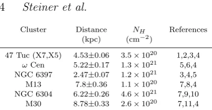
We briefly describe the data used to study each quiescent LMXB, and our best estimates of the distance to each glob-ular cluster. We summarize the key information about these sources in Table1.

2.1 47 Tuc: X7 and X5

47 Tuc is an excellent target due to its relatively short dis-tance, relatively bright quiescent LMXBs, and relatively low

NH (the amount of interstellar gas absorbing soft X-rays).

The core is sufficiently dense with X-ray sources that only

Chandraobservations can fully resolve the sources. The two relatively bright quiescent LMXBs in 47 Tuc, X5 and X7, are bright enough that deepChandra _{observations in 2000}

and 2002 suffered substantial (∼20%) pileup. We therefore obtained 181 kiloseconds of new Chandra _{observations in}

(4)

Cluster Distance NH References

(kpc) (cm−2₎

47 Tuc (X7,X5) 4.53±0.06 3.5×1020 _1,2,3,4

ωCen 5.22±0.17 1.3×1021 _5,6,4 NGC 6397 2.47±0.07 1.2×1021 _3,4,5 M13 7.8±0.36 1.1×1020 _7,8,4 NGC 6304 6.22±0.26 4.6×1021 _7,9,10

M30 8.78±0.33 2.6×1020 _7,11,4

Table 1. List of clusters containing the quiescent LMXBs we analyze, with the best measurements of their distances andNH

columns, and references pertaining to those. References: 1)

Bog-danov et al.(2016), 2) Bergbusch & Stetson(2009), 3)Hansen

et al. (2013), 4) Harris (1996), 2010 update, 5) Heinke et al.

(2014), 6)Bono et al. (2008), 7) Recio-Blanco et al.(2005), 8)

Sandquist et al.(2010), 9)Piotto et al.(2002), 10)Guillot et al.

(2013), 11)Dotter et al.(2010)

X7 and X5; we use those M-R constraints in our combined analysis.

X5 shows eclipses with an 8.67 hour period, and dips, stronger at lower energies, due to varying local extinction (Heinke et al. 2003a). These indicate that X5 is viewed nearly edge-on, so that the companion star eclipses X-rays from the NS, and that material from the dynamic accretion disk is often present along the line of sight.

Bogdanov et al.(2016) also compiled a list of literature determinations of the distance to 47 Tuc, by a variety of methods, and compiles a weighted mean of the distance de-terminations. To limit the effect of flaws in any one method, they conducted “jackknife” tests, where they removed all measurements taken with one method, to assess the system-atic errors, finding a final distance of 4.53+0.08

−0.04 kpc for 47

Tuc.1 _{We use Bogdanov et al’s distance estimate, but}

as-sume symmetric errors, taking 0.06 kpc as the 1-sigma error uncertainty.

2.2 ω Cen

ωCen is a relatively nearby and low-density globular clus-ter, for which eitherChandra orXMM-Newtoncan resolve the known quiescent LMXB. We use Chandra _{data on} _ω

Cen from 2000 (69 kiloseconds) and 2012 (225 kiloseconds), along with the XMM-Newton _{data from 2001 (40}

kilosec-onds), reduced as described byHeinke et al.(2014). It is often easier to establish the relative distance scale of several globular clusters than an absolute scale. We use the well-established relative difference in distances between

ωCen and 47 Tuc (ωCen is 16(±3)% farther than 47 Tuc,

Bono et al. 2008) to calculate the distance to ω Cen as 5.22±0.17 kpc. This is consistent with the horizontal branch distance of 5.2 kpc ofHarris(1996)2_{, the dynamical distance}

estimate of 5.19+0₋₀._.07₀₈kpc ofWatkins et al.(2015), and in the middle of the other distance estimates discussed byHeinke et al.(2014).

1 _{Bogdanov et al.}₍₂₀₁₆_{) also addressed the discrepancy with the}

dynamical distance estimate of Watkins et al. (2015), showing why Watkins’ value is discrepant, and noting that when Watkins et al. use a larger dataset, the discrepancy disappears.

2 _{http://physwww.physics.mcmaster.ca/}_∼_{harris/mwgc.dat}

2.3 NGC 6397

NGC 6397 is the second nearest globular cluster, with a very dense core. We useChandra_{observations taken in 2000 (49}

kiloseconds), 2002 (55 kiloseconds), and 2007 (240 kilosec-onds), reduced as described byHeinke et al.(2014) (similar toGuillot et al.(2011)).

As forωCen, we use the relative distance measurements to NGC 6397 and 47 Tuc (that NGC 6397 is at 54.5±2.5% of 47 Tuc’s distance,Hansen et al.(2013)) to calculate NGC 6397’s distance at 2.47±0.07 kpc. This is in agreement with the dynamical distance estimate of 2.39+0.13

−0.11kpc ofWatkins et al.(2015), and with most other recent distance estimates discussed inHeinke et al.(2014).

2.4 M13

M13 is a relatively low-density cluster with very low extinc-tion. It was the subject of extensive ROSAT observations (46 kiloseconds) in 1992 with the PSPC camera, which accu-rately measured the absorption of the low-energy spectrum (though ROSAT has much poorer spectral resolution in gen-eral). We use this ROSAT PSPC spectrum, 2002 XMM-Newton _{observations (34.6 kiloseconds), and 2006} Chan-draobservations (54.7 kiloseconds), reduced as described by

Catuneanu et al.(2013) (similar toWebb & Barret(2007)). The distance to M13 has been extensively discussed by

Sandquist et al. (2010), who estimate 7.65±0.36 kpc (rec-onciling distance estimates using the tip of the red giant branch with horizontal branch estimates), while the homo-geneous relative distance estimates of Recio-Blanco et al.

(2005) (which perfectly matches our distance estimate to 47 Tuc) gives a distance of 7.8±0.1 kpc. We use Recio-Blanco’s distance, but conservatively use the larger distance uncer-tainty, 7.8±0.36 kpc.

2.5 NGC 6304

The quiescent LMXB in NGC 6304 is located in the core of its cluster near other sources (Guillot et al. 2009b), so we use only the deep Chandra _{observation of 2010 (98.7}

kiloseconds), extracted followingGuillot et al.(2013), using CIAO 4.7 and CALDB 4.6.9.

The distance to NGC 6304 is uncertain due to its rela-tively high extinction, and thus high uncertainty on its ex-tinction. Using the distance modulus ofRecio-Blanco et al.

(2005) and the extinction estimate of Piotto et al. (2002) (followingGuillot et al. 2013) gives a distance of 6.22±0.26 kpc.

2.6 M30

The quiescent LMXB lies in the extremely dense core of the distant, but low-extinction, globular cluster M30, and can only be resolved byChandra. We use the 2001Chandra

observation (49 kiloseconds), and extract the data following

Lugger et al.(2007) (alsoGuillot & Rutledge 2014), using CIAO 4.7 and CALDB 4.6.9.

(5)

for 47 Tuc, we adopt this. We note that it is also in agree-ment with other estimates by, e.g.,Dotter et al.(2010) (8.8 kpc).

2.7 M28

The quiescent LMXB in M28 (source 26 of Becker et al. 2003) lies in the core of this relatively nearby, dense clus-ter. We use threeChandra observations from 2002 (42 kilo-seconds) and two from 2008 (199.6 kilokilo-seconds), reduced as described inServillat et al.(2012), using CIAO 4.7 and CALDB 4.6.9.

We use the estimate of the distance to M28 of 5.5±0.3 kpc, derived from the brightness of the horizontal branch (Testa et al. 2001) calibrated byHarris(1996, 2010 revision).

3 X-RAY SPECTRAL FITTING

For the spectral fitting, we used the XSPEC software ( Ar-naud 1996). We experimented with merging spectra taken with the same detector close in time, or fitting them simul-taneously; with grouping the data into bins of >20,>50, or other numbers of counts; with analyses using χ2 _or

C-statistics. In general, such changes do not make substantial differences to the final results.

For all spectra, our spectral fits included a neutron star atmosphere, either NSATMOS (hydrogen,Heinke et al. 2006a) or NSX (helium, Ho & Heinke 2009). We included

NH through the TBABS model (with the extinction free to

vary), using element abundances from Wilms et al.(2000) and photoelectric cross-sections from Verner et al. (1996). We include a power-law in the spectral fitting, although it is not required for any quiescent LMXB, with the pho-ton index fixed to 1.5, as typical for power-law components in quiescent LMXBs (Campana et al. 1998; Cackett et al. 2010;Chakrabarty et al. 2014). We add systematic errors, of magnitude 3%, to all spectra, accounting for instrumen-tal calibration uncertainties, followingGuillot et al.(2013);

Bogdanov et al. (2016). Our spectral fits were performed assuming the nominal best-fit distances, with distance un-certainties convolved with the probability density functions (from the spectral fits) during the Bayesian MCMC calcu-lation (see below).

Bogdanov et al.(2016) found that the inclusion of pileup in spectral modelling forChandra _{observations of X7 in 47}

Tuc made a significant difference to the final radius contours, even at pileup fractions as low as 1%. For this reason, we include pileup in allChandraspectral fits; this is particularly relevant for the NGC 6397 spectral fits, since previous fits (Guillot et al. 2013;Heinke et al. 2014) did not include pileup for this source. The M28 quiescent LMXB has the highest fraction of piled-up events, with about 5% of photons piled up (Servillat et al. 2012).

A crucial uncertainty is the chemical composition of the atmosphere of the quiescent LMXB. In the Bayesian MCMC analysis below, we analyze the spectra of each qui-escent LMXB with both hydrogen and helium atmospheres with two exceptions. The first exception is the quiescent LMXBωCen which has a firm detection of hydrogen in its spectrum (Haggard et al. 2004). The second is X5, which

has a long orbital period (Heinke et al. 2003a) suggesting a hydrogen-rich donor (see section1.2).

3.1 Systematic Uncertainties

There are remaining systematic uncertainties which we have not robustly controlled. Perhaps the largest uncertainty is the possible effect of hot spots upon the inferred radius. Many neutron stars show pulsations, implying the presence of hotter regions on their surface; examples include young pulsars (De Luca et al. 2005), old millisecond pulsars ( Bog-danov 2013), young neutron stars without pulsar activity (Gotthelf et al. 2010), and accreting neutron stars (Patruno et al. 2009). Hot spots may be produced by the accretion of material onto a magnetic pole, collision of relativistic elec-trons and posielec-trons with the pole during pulsar activity, or preferential leakage of heat from the core along paths with particular magnetic field orientations (Potekhin & Yakovlev 2001). Elshamouty et al. (2016) explored the effect of hot spots on quiescent LMXB spectra, focusing on the cases of X7 and X5 in 47 Tuc. Elshamouty et al. used deepChandra

observations at high time resolution to search for pulsations from these two sources. Considering a range of possible mag-netic latitudes and inclinations, they derived limits on the hot spot temperature, and then derived limits on the bias that might be inferred by fitting a single-temperature neu-tron star atmosphere to a neuneu-tron star that has hot spots. Unfortunately, existing data poses only weak limits, such that the spectroscopically inferred radius could be biased downwards up to 28% smaller than the true radius. We will consider biases up to this level in some of our analyses.

Another concern is variability in the absorbing column. As mentioned above, X5 in 47 Tuc is a nearly edge-on sys-tem that shows varying photoelectric absorption.Bogdanov et al.(2016) shows that if periods of enhanced absorption (signified by dips in the count rate) are removed, the inferred radius of X5 grows significantly. When time periods includ-ing different absorption values are combined and fitted with a single absorber, the spectrum appears intrinsically more curved (and thus at a hotter temperature). However, we can-not be sure that we have removed all the periods of enhanced photoelectric absorption; short periods of enhanced absorp-tion would not supply enough counts to enable unambiguous determination of a dip. We thus suspect that the spectral fits to X5 may be biased downwards by varying photoelec-tric absorption. This problem might affect other quiescent LMXBs as well. Though no other quiescent LMXB among our sample shows eclipses, absorption dips have been seen in LMXBs that are not seen edge-on (cf.Galloway et al. 2016

andMata S´anchez et al. 2016), although to date these dips have only been seen during outburst.

4 BAYESIAN INFERENCE FOR NEUTRON

STAR MASSES AND RADII

(6)

bins for each neutron star data set. In this work, we con-vert the X-ray spectrum for each source into a probability distribution for the neutron star with radiusR, massM, at distanceDwith atmosphere compositionX

D(R, M, D, X) = exp

−χ2(R, M, D, X)/2

(1)

In essence, this exponential of a sum is equivalent to a prod-uct over Gaussians for each energy bin for the X-ray spec-trum which is fit.

Note that this assumes that the uncertainties between energy bins in the spectrum and uncertainties between ob-jects are both uncorrelated. This may not be the case, as sys-tematic uncertainties in a particular observation may affect a number of high-energy X-ray bins. Also,XMM-Newton ob-servations may have uncorrected systematics which are dif-ferent than those from Chandra. Such systematics are be-yond the scope of the current work, except for the 3% un-certainty which we added to all of the spectra as described above (see, e.g.,Lee et al. 2011;Xu et al. 2014for potential future directions).

From the eight probability distributions for each neu-tron star, we can directly apply a generalization of the ap-proach first described inOzel & Psaltis¨ (2009),Steiner et al.

(2010), andOzel et al.¨ (2010). FollowingSteiner et al.(2010) we employ Bayesian inference and we assume uniform prior distributions unless otherwise specified below. Upper and lower limits for uniform distribution for the model parame-ters,{pi}, are chosen to be extreme enough that they do not

affect the final results. The posterior probability distribution for quantityQis then

PQ(q) ∝

Z (M Y

i=1

Di[R(Mi,{pj}), Mi, Di, Xi] )

×δ[q−Q(p1, . . . , pN, M1, . . . , MN,

D1, . . . , DN, X1, . . . , XN)] ×dp1 . . . dpN dM1. . . dMN

×dD1. . . dDN dX1. . . dXN, (2)

where N is the number of neutron stars being considered. Several examples of relevant posteriors are reviewed briefly inLattimer & Steiner(2014a).

We assume the composition, Xi of the atmosphere of

each neutron star (except for the neutron star inωCen and for X5 in 47 Tuc) is a discrete binary variable: either H or He. As a prior distribution we assume a 2/3 probability of H and a 1/3 probability of He, following the observed ratio of H-rich to He-rich donors in bright LMXBs in globular clus-ters (Bahramian et al. 2014, and references therein). This method is superior to that employed inLattimer & Steiner

(2014b) because it allows us to quantitatively predict the posterior probability that any particular neutron star has a H or He atmosphere. On the other hand, it has been argued by some authors that helium atmospheres are expected to be unlikely (Guillot & Rutledge 2014), so we also try mod-els where the prior probability for hydrogen is 90% or 100%. We remove the neutron star in X5 from our baseline data set because of the varying absorption described in section3.1. We assume the maximum mass must be larger than 2 M⊙

as implied by the recent observations of high mass neutron stars (Demorest et al. 2010;Antoniadis et al. 2013). We al-low neutron stars to have masses as al-low as 0.8 M⊙ (which

may be conservative), but increasing this number has little effect on our results.

As discussed inBogdanov et al.(2016) (see also Bezno-gov & Yakovlev 2015), there are strong reasons to believe that these neutron stars are not close to 2 M⊙ in mass,

since that would likely produce extremely rapid cooling (by processes such as direct Urca, e.g.Yakovlev et al. 2003) so that we would not observe strong thermal radiation from their surfaces. This method is potentially powerful to con-strain the masses of neutron stars, but at this time the mass at which rapid cooling turns on is not well-constrained. The neutron star in SAX J1808.4-3658 is extremely cold, indicat-ing that rapid coolindicat-ing processes are active (e.g.Heinke et al. 2009). This neutron star seems not to have a particularly large mass (the 2σ upper limit on the mass is ∼1.7 M⊙),

though current constraints are not very strong (Wang et al. 2013).

4.1 Distance and Hotspot Correction

In this work, we choose to marginalize over the distance as a nuisance variable instead of producing a separate fit for each distance. So long as all of the probability distributions of in-terest (all of the quantitiesPQin eq.2above) are

indepen-dent of distance, we can perform the distance integrations first. This means that we cannot generate any posterior dis-tributions for the distance, but we expect other methods to provide superior distance measurements anyway.

In units wherec= 1, there is a bijection between (R, M) and (R∞, z) whenR >2GM (the composition will be

con-sidered later and is thus suppressed for now):

R∞(R, M) =R

1−2GM_R −1/2

(3)

and

z(R, M) =

1−2GM_R −1/2

−1. (4)

The opposite transformation is given by

M(R∞, z) =

R∞

G

_z_{(2 +}_z₎

2(1 +z)3

(5)

and

R(R∞, z) =

R∞

(1 +z). (6) To first order (adequate for small fractional uncertain-ties), distance scales withR∞. Thus to correct for a variation

in distance,D=Dnew±δDkpc given an original

probabil-ity distributionDold(R, M) based on a fixed distance,Dold,

we compute

Dnew( ˆR,Mˆ) =

Z ∞

0

dRˆ∞

"

Dold

R∞( ˆR,Mˆ)δD

√

2π

#

exp



 

  −

h

ˆ

R∞−R∞( ˆR,Mˆ)Dnew/Dold

i2

2hR∞( ˆR,Mˆ)δD/Dold

i2 

 

 

×Dold{R[ ˆR∞, z( ˆR,Mˆ)],

M[ ˆR∞, z( ˆR,Mˆ)]}. (7)

(7)

9 10 11 12 13 14 15 16 6304, H atm., w/dist. unc.

0.0

6304, H atm., w/dist. unc.

0.0

Figure 1.This figure is a demonstration of the incorporation of the distance uncertainty as in Eq.7. The original mass-radius probability distribution (arbitrary normalization) for a neutron star in NGC 6304 including a 3% systematic uncertainty and X-ray absorption assuming abundances fromWilms et al.(2000) is in the upper-left panel. The probability distribution is converted to (R∞, z) space (upper-right panel), and then shown again in the lower-left panel after an integration over a Gaussian distance uncertainty. The lower-right panel shows the result after the con-version back to (M, R) space. The probability distribution in the lower right panel smoothly falls off at the edges, but this is will not affect our final results.

0, then the exponential and associated normalization is equal to a delta function,

h _D

so in this limit

Dnew( ˆR,Mˆ) = Dold{R[R∞( ˆR,Mˆ)Dnew/Dold, z( ˆR,Mˆ)],

M[R∞( ˆR,Mˆ)Dnew/Dold, z( ˆR,Mˆ)]}. (9)

If Dnew = Dold, the term on the right-hand side of Eq. 9

just becomesDold( ˆR,Mˆ) (i.e. the probability distribution is

unchanged). Finally, Eq.7also ensures that the new relative uncertainty inR∞is equal toδD/Dnew, since

δRˆ∞

Fig.1gives a demonstration of the method. The distri-bution is transformed to (R∞, z) space (upper-right panel)

where the distance uncertainty is applied (lower-left panel), and then transformed back to (R, M) space (lower-right panel).

Alternatively, we can rescale R at constant z and ob-tain the same distributionDnew. To show this, create a new

dummy integration variable, R ≡ Rˆ∞/[1 +z( ˆR,Mˆ)]. The 6304, H atm., w/dist. unc.

0

6304, H atm., w/dist. unc.

0.0

6304, H atm., Wilms et al. abun., hotspot

0

Figure 2.Upper left and upper right panels: A demonstration of the distance uncertainty having been applied in (R, z) space as implied by Eq.11. The final result, in the lower left panel, is the same as that in the lower-right panel of Fig.1. Lower right panel: A demonstration of the effect of a hotspot, to be compared with the lower right panel in Fig.1.

value z( ˆR,Mˆ) is independent of the integration variable,

R, so dR/dRˆ∞ = 1/[1 +z( ˆR,Mˆ)]. Since R∞( ˆR,Mˆ)/[1 +

z( ˆR,Mˆ)] = ˆR, the integral on the right-hand side of Eq.7

can be rewritten to give

Dnew( ˆR,Mˆ) =

Note that, in the figures below, the rescaled results from either Eqs.7or 11shows that the probability distribution vanishes at the extremes inM and R. This is because we must assume the input probability distributions from the X-ray fits are step functions (e.g. they drop immediately to zero probability forR <9 km) and these step functions are softened by the additional distance uncertainty.

A demonstration of the method implied by Eq.11, ap-plied to the neutron star in NGC 6304 is given in the upper panels of Fig.2. The final result (not shown) is indistinguish-able from the lower right panel in Fig.1. The final results, given by Eq.7, for the baseline data set and for X5 in 47 Tuc assuming a H atmosphere are presented in Fig.3. The effect of an He atmosphere on the neutron stars (except for X5 and the neutron star inωCen) in Fig.4.

(8)

param-10 12 14 16

Figure 3.The H atmosphere part of our baseline data set plus the neutron star X5 in 47 Tuc. The Wilms et al.(2000) abun-dances are used to correct for X-ray absorption in all cases, the normalization is arbitrary, and a distance uncertainty has been added following the prescription described in section4.

eter which increases R∞ by a fixed percentage in order to

compensate for this effect. We presume that this parame-ter has a uniform prior distribution and take its value to be between 0% and 28%. As an example, the probability distri-bution for the neutron star in NGC 6304 after having made this correction is given in the lower right panel of figure2. The final data set presuming a possible hotspot with hydro-gen atmospheres is in Fig.5 and with helium atmospheres (where appropriate) is in Fig.6.

10.0 12.5 15.0 17.5 20.0

Figure 4.Left panel: The mass and radius constraints for the neutron stars in our data set when a He atmosphere is assumed (compare with Fig. 3). Our baseline model includes He atmo-spheres for all neutron stars except those inωCen and X5.

4.2 Equation of State

Quantum Monte Carlo calculations of neutron matter ( Gan-dolfi et al. 2012) provide an excellent description of matter up to the nuclear saturation density (ρ≈2.8×1014_g_/_cm3_).

As inSteiner et al.(2015), we assume that neutron star mat-ter near the saturation density is described by results from quantum Monte Carlo. We also assume the neutron star has a crust as described in Baym et al. (1971) and Negele & Vautherin(1973).

(9)

10 12 14 16

Figure 5.The H atmosphere part of our baseline data set plus the neutron star X5 in 47 Tuc assuming a hotspot may be present.

TheWilms et al. (2000) abundances are used to correct for

X-ray absorption in all cases, the normalization is arbitrary, and a distance uncertainty has been added following the prescription described in section4.

uses line-segments in pressure and energy density space and makes stronger phase transitions more likely. It is impor-tant to emphasize that the ability of the parameterization to describe a generic EOS is not the only consideration (as both polytropic models and those based on line segments can reproduce almost all EOSs). Once a parameterization and a prior for the parameters is specified, changes in the likelihood with which various EOSs are selected can make a significant change in the results. We present results from these two high-density EOSs separately and assign an equal prior probability to each. We use the open-source code from

Steiner (2014a,b) to perform the simulations which have

10.0 12.5 15.0 17.5 20.0

Figure 6.Left panel: The mass and radius constraints for the neutron stars in our data set when a hotspot and a He atmosphere is assumed (compare with Fig.3). Our baseline model includes He atmospheres for all neutron stars except those inωCen and X5.

been updated to use affine-invariant sampling (Goodman & Weare 2010).

5 RESULTS

Ideally, one decides the prior distribution before any cal-culations are performed. We assign all the different models and interpretations of the data (described in detail below) equal probability. Thus our full posteriors can be viewed as the sum over the results presented for each individual model and/or data interpretation (after having been prop-erly weighted by their evidence).

(10)

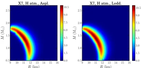
abundance models, we compare our mass and radius distri-butions derived using the Wilms et al. (2000) abundance model to those derived using the abundance models of As-plund et al. (2009) and Lodders (2003). These abundance models, produced using studies of the Sun and meteorites, respectively, suggest a plausible range of uncertainty for the interstellar abundances. This is in contrast to significantly older abundance models such as those ofAnders & Grevesse

(1989), which are quite different, and would lead to signifi-cant changes to radius estimates (Heinke et al. 2014). Fig.7

shows the mass and radius constraints for X7 in 47 Tuc using these alternate abundance models and demonstrates that the results are only slightly different (differences in in-ferred radius are less than 1%, in agreement withBogdanov et al. 2016from those usingWilms et al.(2000) abundances. This holds for all of the objects in our data set, so we only present results using Wilms et al. (2000) abundances be-low. We have also tested the effects of the updated tbnew

code by J¨orn Wilms3, and find that the code improvements oftbnew_{(mostly fine structure around edges, affecting}

high-resolution spectroscopy) affect radius estimates on the order of 0.1%.

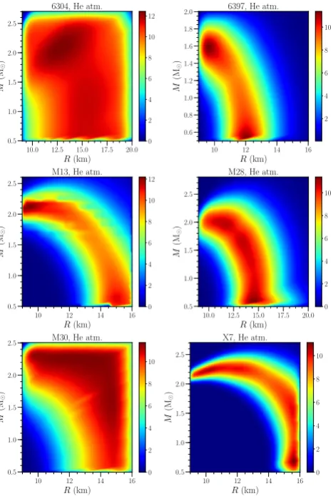
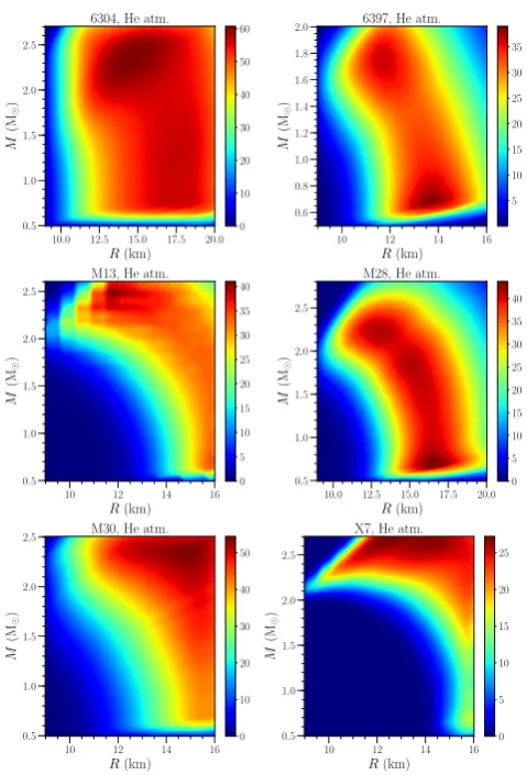
The posterior mass and radius distributions for the neu-tron stars in the baseline scenario are given in Fig. 8, to-gether with the results presuming Model C is used for the EOS. The mass posterior distributions are relatively broad, with the sole exception for X7. The mass of X7 must be larger than 1.1 M⊙in Model C because smaller mass stars

have central densities too low to allow for the phase tran-sition to decrease the radius sufficiently to match the mass and radius implied by the observations.

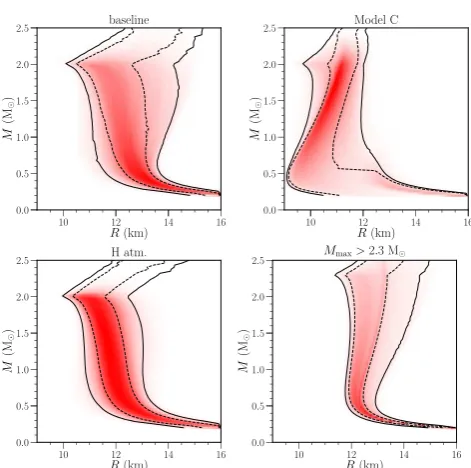
The upper left panel of Fig. 9 shows an ensemble of one-dimensional radius histograms for a fixed mass. The re-sults imply that the radius for aM = 1.4 M⊙neutron star

is between 11.0 and 14.3 km (to 95% confidence; see Ta-ble2). The figure gets less dark at higher mass because the area under a radius histogram at fixed mass is normalized to the probability that the maximum mass is larger. Note that the probabilities shift towards larger radii for masses above 2 M⊙ because larger mass stars require a larger maximum

mass, which in turn requires a larger pressure at lower den-sities and thus a larger radius. The probabilities for a helium atmosphere for each source are given in Table3and strongly prefer a He atmosphere for the neutron star in NGC 6397 and a H atmosphere for the neutron star X7 in 47 Tuc. Note that the probability of a He atmophere hovers around 1/3 for objects like the neutron star in NGC 6304 and that in M30 since the probability distributions for those two objects are too broad to allow a strong constraint on the atmosphere composition (as shown in Fig.1and Fig.3).

A significant decrease in the radius comes from using a model of high-density matter which allows for strong phase transitions, as found in Steiner et al. (2013, 2015). This causes likely radii for M = 1.4 M⊙ neutron stars to drop

by 1 to 2 km (see also upper right panel of Fig. 9). The probabilities for helium atmospheres drop significantly for some objects, including the neutron star in NGC 6397, the neutron star in M13, and X7 in 47 Tuc. Assuming all neutron stars must have a hydrogen atmosphere (lower left panel of

3 _{http://pulsar.sternwarte.uni-erlangen.de/wilms/research/tbabs/}

9 10 11 12 13 14 15 16

R(km)

0.5 1.0 1.5 2.0 2.5

M

(M

⊙

)

X7, H atm., Aspl.

0.0 1.5 3.0 4.5 6.0 7.5 9.0 10.5

9 10 11 12 13 14 15 16

R(km)

0.5 1.0 1.5 2.0 2.5

M

(M

⊙

)

X7, H atm., Lodd.

0.0 1.5 3.0 4.5 6.0 7.5 9.0 10.5

Figure 7.Left panel: The mass and radius constraints for the neutron star 47 Tuc in X7 when a H atmosphere is assumed and

Asplund et al. (2009) abundances are used (compare with the

lower right panel in Fig.3). Right panel: The mass and radius constraints for the neutron star 47 Tuc in X7 when a H atmo-sphere is assumed andLodders(2003) abundances are used.

Fig.9) also decreases the 95% confidence limits in the radius by 0.2 (lower bound) and 1.3 km (upper bound). Requiring the neutron star maximum mass to lie above 2.3 M⊙

in-creases the lower limit for the radius by 0.7 km (lower right panel of Fig.9), similar to the result found inSteiner et al.

(2013,2016).

Constraining the mass of the neutron stars (to either 1.3−1.7 M⊙, or to 1.3−1.5 M⊙) also has relatively little

ef-fect on the inferred radii as shown in the upper left and upper right panels of Fig.10. If we include X5 in our data set (lower left panel of Fig.10), then radii above 13.9 km for aM = 1.4 M⊙neutron star are strongly ruled out. The

lower limit for the radius decreases, but only slightly, as radii smaller than about 11 km require a strong phase transition which are disfavored in polytropic models. In this case, the preference for a helium atmosphere decreases in objects for which the probabilities are not dominated by the prior choice (which tends to be those stars which have posterior proba-bilities not near 33%). The model permitting hotspots sig-nificantly increases the 1σrange for the radius (lower right panel of Fig.10), but has little effect on the 2σlimits (Ta-ble2). The effect of the hotspot on the posterior probability for the atmosphere is most dramatic for the neutron star in NGC 6397 (see table 3). In this case, the hotspot ef-fectively increases the inferred radius, and this makes the H atmosphere more probable, thus decreasing the posterior probability for a He atmosphere by almost a factor of two.

In the baseline model, we assume a 2/3 prior probability that each neutron star has a hydrogen atmosphere. Increas-ing this prior to 90% decreases the posterior probability as seen in the last column of table3, and the effect of this prior choice on the posterior probability is stronger than our other model choices. The effect on the neutron star radius is more modest, as shown in the last row of Table2.

(11)

9 10 11 12 13 14 15

Figure 8. Contour lines representing 68% and 95% confidence limits for the 7 objects in the baseline model (black curves) and with Model C (blue curves). Most of the results appear similar except for X7 which has a bimodality resulting from the choice between H and He atmospheres which is only evident in this neu-tron star because the radius is sneu-trongly constrained.

evidence is computed by rescaling the distinct model pa-rameters which have dimensionful units so that they are in the range [0,1]. The neutron star mass parameters need no rescaling; it is important that they are not rescaled in or-der to properly evaluate the Bayes factor for the models which constrain the neutron star mass more than the base-line model. Bayes factors between 1/3 and 3 are generally regarded as relatively weak, and in this case no definitive statement can be made about the two models.

Requiring all neutron stars to have a H atmosphere is ruled out with a Bayes factor of 1/3, but again as described above this result will strongly depend on the prior

probabil-10 12 14 16

Figure 9.Probability distributions for radii as a function of mass for the baseline data set and baseline model (upper left panel), for the baseline data set with Model C (upper right), the baseline model and assuming H atmospheres (lower left), and the baseline model and baseline data set requiringMmax > 2.3 M⊙ (lower right).

(12)

R(M= 1.4 M⊙) (km) Lower limits Upper limits

Model 95% 68% 68% 95%

baseline 11.03 11.40 13.11 14.28 Model C 9.995 10.40 11.23 11.93 H atm. 10.78 11.20 12.26 13.03

Mmax≥2.3 11.95 12.09 12.98 13.94 1.3< M <1.5 11.02 11.22 13.04 14.44 1.3< M <1.7 11.01 11.30 13.68 14.41 with X5 10.88 11.32 12.78 13.87 hotspot 11.04 11.97 13.62 14.40 90% H 10.85 11.28 12.82 14.03

Table 2.Two-sigma confidence limits for the radius of a 1.4 M⊙ neutron star (in km) for the different combinations of data sets and model assumptions used in this work.

Source Probability of He

baseline w/X5 Model C hotspot 90% H

NGC 6304 32 % 32 % 30 % 31 % 9.1%

NGC 6397 81 % 79 % 47 % 41 % 34 %

M13 28 % 26 % 19 % 26 % 7.0%

M28 52 % 48 % 31 % 33 % 16 %

M30 31 % 30 % 27 % 31 % 8.7%

X7 16 % 2.5% 3.4% 13 % 2.0%

Table 3. Probability of a Helium atmosphere for each neutron star depending on data set and model assumptions. The statistical uncertainties in these probabilities are about 3%.

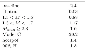
Data and model selection Evidence

baseline 2.4

H atm. 0.68

1.3< M <1.5 0.88 1.3< M <1.7 1.17

Mmax≥2.3 1.0

Model C 20.2

hotspot 1.4

90% H 1.8

Table 4.The evidence, as computed by the properly normalized integral under the posterior distribution, for the different combi-nations of data sets and model assumptions used in this work.

ity of a H atmosphere. Constraining the neutron star mass to between 1.3 and 1.7 M⊙ drops the evidence by a

fac-tor of 2 and further constraining it to between 1.3 and 1.5 M⊙drops the evidence by an additional 30 percent.

Assum-ing the presence of hotspots drops the evidence by a factor of two. In agreement with previous work, we find that the choice of EOS model has a strong impact (see e.g. Steiner et al.(2015)). We find that the Model C is strongly preferred over the baseline result (a Bayes factor of 8.4). One way of diagnosing which object contributes most strongly to this improved fit is by looking at the ratio of the average pos-terior probability for each object between Model C and the baseline result. These ratios are 1.03, 2.24, 1.03, 1.39, 0.94, 1.29, and 1.86 for the neutron stars in NGC 6304, NGC 6397, M13, M28, M30,ωCen, and for X7 in 47 Tuc, respectively. (The product of these ratios is not exactly equal to 8.4 be-cause of correlations between the weight from each neutron star). Thus the neutron star in NGC 6397 most strongly pushes the results towards smaller radii, followed by X7 and

0 500 1000 1500

−0.5

0.0 0.5 1.0 1.5 2.0 2.5 3.0

log

10

P

(MeV

/

fm

3)

ε(MeV/fm3₎

baseline

0 500 1000 1500

−0.5

0.0 0.5 1.0 1.5 2.0 2.5 3.0

log

10

P

(MeV

/

fm

3)

ε(MeV/fm3₎

Model C

0 500 1000 1500

−0.5

0.0 0.5 1.0 1.5 2.0 2.5 3.0

log

10

P

(MeV

/

fm

3)

ε(MeV/fm3₎

H atm.

0 500 1000 1500

−0.5

0.0 0.5 1.0 1.5 2.0 2.5 3.0

log

10

P

(MeV

/

fm

3)

ε(MeV/fm3₎

Mmax>2.3 M⊙

Figure 11.A set of posterior distributions for the pressure at fixed energy density over a range of energy densities for some of the models used in this work. The upper left panel shows results for our baseline model, the upper right shows the results for Model C, the lower left assumes H atmospheres for all sources and the lower right assumes a maximum mass larger than 2.3 M⊙.

then by the neutron star in M28. There is no standard ap-proach to computing the Bayes factor when the data sets are different, so we cannot evaluate whether or not including X5 is more or less consistent with our model assumptions.

The posteriors for the relation between energy density and pressure are presented in Fig. 11. This figure shows a set of pressure histograms at fixed energy density, normal-ized to the probability that the central energy density in the maximum mass star is larger than the specified energy den-sity. Thus the plot becomes less dark towards higher energy densities because they are often higher than the maximum. The upper left panel shows our baseline results. The plot is darker near 800 MeV/fm3 because that energy density is more strongly constrained than near theε= 400 MeV/fm3_.

The strongest deviation from the baseline model is for Model C, where the EOS parameterization allows for large regions where the pressure is flat. These phase transitions occur at rather low densities to match the stars which have smaller inferred values ofR∞ and the pressure increases strongly

above the phase transition in order to ensure that the max-imum mass is above 2 M⊙. The lower left panel assumes

H atmospheres, leading to a smaller pressure in the range of energy densities from 300 to 500 MeV/fm3_{. Increasing}

the maximum mass, shown in the lower right panel, has the opposite effect. In the lower right panel, the central energy density of the maximum mass star decreases significantly, as one expects when increasing the maximum mass. Note that, since the posterior mass for the neutron stars in our data set is not often near 2 M⊙, our constraint on the EOS at high

(13)

Lower limits Upper limits

Model 95% 68% Most prob. 68% 95%

P(ε= 300 MeV/fm3_{) (MeV}_/_fm3₎

baseline 7.202 11.38 15.81 23.42 38.17 with X5 7.200 11.41 15.63 20.55 33.36 Model C 1.830 2.039 2.851 8.621 14.47 H atm. 7.233 11.36 14.10 17.33 23.49

Mmax>2.3 14.12 15.46 17.20 25.05 48.72 1.3< M <1.5 6.265 10.44 15.45 21.61 48.92 1.3< M <1.7 6.427 9.766 15.55 23.58 47.80 hotspot 8.625 13.22 17.35 27.87 44.01 90% H 7.083 11.24 15.52 20.32 34.02

P(ε= 450 MeV/fm3_{) (MeV}_/_fm3₎

Mmax>2.3 59.92 66.99 73.30 113.6 132.0 1.3< M <1.5 30.12 39.68 48.93 74.57 117.5 1.3< M <1.7 30.37 38.95 47.83 75.55 118.1 hotspot 40.14 49.62 71.14 86.97 114.6 90% H 33.03 41.12 48.65 70.25 87.11

P(ε= 600 MeV/fm3_{) (MeV}_/_fm3₎

Mmax>2.3 147.4 157.8 184.7 202.1 254.3 1.3< M <1.5 86.88 98.81 119.6 144.7 196.3 1.3< M <1.7 86.03 97.40 118.6 143.8 201.1 hotspot 97.57 108.9 125.4 157.8 197.5 90% H 88.30 103.6 117.8 135.7 158.0

P(ε= 1000 MeV/fm3_{) (MeV}_/_fm3₎

Mmax>2.3 299.3 342.2 389.4 460.8 530.8 1.3< M <1.5 247.0 298.8 331.2 382.9 497.2 1.3< M <1.7 243.7 298.1 328.3 382.5 494.7 hotspot 243.3 292.7 341.0 407.5 487.1 90% H 254.3 296.8 316.6 364.6 408.5 Table 5. Constraints on the pressure at four energy densities in the various model and data set choices used in this work. Note, in particular, the strong variation in the pressure at ε= 300 MeV/fm3_{which is about twice the nuclear saturation density.}

The neutron star central baryon density is an impor-tant parameter for understanding the extent to which nu-clear physics can play a role in neutron star structure. We find that the central baryon density of the maximum mass star could be as low as 4 times the nuclear saturation den-sity, n0 = 0.16 fm−3 or as large as 8n0, in agreement with Steiner et al.(2015). The masses and radii for neutron stars which have central baryon densities equal to integer multi-ples of n0 are shown in Fig.12. The left panel shows our

results for the baseline model and the right panel shows the results for Model C. This figure is an updated version of Fig. 2 fromGandolfi et al.(2012) which properly quantifies the uncertainty in the result by removing the unwarranted

10 12 14 16 18 20 0.0

0.5 1.0 1.5 2.0 2.5

R(km)

M

(

M

⊙

)

nB,cent=n0

nB,cent= 2n0

nB,cent= 3n0

nB,cent

= 5n0

Baseline

30< L <40 MeV

60< L <70 MeV

10 12 14 16 18 20 0.0

0.5 1.0 1.5 2.0 2.5

R(km)

M

(

M

⊙

)

nB,cent=n0

nB,cent= 2n0

nB,cent= 3n0

nB,cent= 5n0

Model C

30< L <40 MeV

60< L <70 MeV

Figure 12.A plot showing the mass and radii of neutron stars which have a central baryon density equal to an integer multiple of the nuclear saturation density,n0 = 0.16 fm−3. The results are separated into different assumptions about the slope of the symmetry energy,L. The left panel shows the baseline model and the right panel shows the results from Model C.

assumption that matter at high densities can be described by the same Hamiltonian which is used at the nuclear satu-ration density. The relationship with the density derivative of the symmetry energy,L is also shown. It is standard to write the energy densityε(nB, δ) as a function of the neutron

and proton number densities,nn and np, using the

defini-tionsnB =nn+nP andδ= 1−2np/nB. Then the quantity

Lis defined by

L≡3nB ∂

∂nB

1 2nB

∂2ε ∂δ2

. (12)

Lattimer & Prakash (2001) showed that for a set of typ-ical models L is correlated with the radius of a 1.4 solar mass neutron star. However, this correlation is weak if one assumes a prior probability which allows for strong phase transitions in the EOS (Steiner et al. 2016) as also shown in Fig. 12. The lower and upper limits for the value of L

and for the radii of higher mass stars for all nine scenarios is given in Table6.

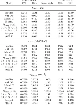
The one- and two-sigma limits for the radius of the max-imum mass neutron star are given in Table 7. The most extreme radii are observed if the EOS at high densities is assumed to have strong phase transitions, in which case the two-sigma limit goes below 9.4 km. Larger lower limits occur if the maximum mass is greater than 2.3 M⊙or if the

neu-tron stars have uneven temperature distributions, otherwise the lower two-sigma limit is typically around 9.7 km. Ta-ble7also presents the limits for the central baryon (ranging from 0.61 to 1.3 fm−3_{) and energy density (ranging from 740}

to 1700 MeV/fm3). Increasing the maximum mass tends to decrease these central densities significantly.

6 DISCUSSION

Steiner et al.(2013) found radii between 10.4 and 12.9 km (to 95% confidence) for a 1.4 M⊙neutron star, and our

(14)

Lower limits Upper limits

L(MeV)

Mmax>2.3 30.21 30.31 30.72 33.66 40.23 1.3< M <1.5 30.59 40.56 49.79 59.87 69.41 1.3< M <1.7 30.97 40.88 50.97 58.87 69.41 hotspot 34.47 40.91 48.19 61.62 69.55 90% H 32.50 41.77 51.85 57.59 64.48

R(M= 1.7 M) (km)

Mmax>2.3 11.95 12.13 13.06 13.16 14.25 1.3< M <1.5 10.80 10.99 11.76 12.81 14.64 1.3< M <1.7 10.76 10.88 11.90 13.85 14.62 hotspot 11.18 11.78 12.69 13.67 14.58 90% H 10.71 11.06 11.73 12.59 13.99

R(M= 2.0 M) (km)

Mmax>2.3 11.84 12.07 13.21 13.30 14.50 1.3< M <1.5 10.08 10.32 11.16 12.57 14.81 1.3< M <1.7 10.09 10.20 11.08 12.72 14.85 hotspot 10.54 11.28 12.45 13.58 14.67 90% H 9.996 10.40 11.00 12.12 13.62 Table 6.Constraints on the derivative of the symmetry energy and the radii of 1.7 and 2.0 M⊙ neutron stars for the nine sce-narios explored in this work.

km to 95% confidence. One could conceive of many possible combinations among the model assumptions which we have explored. For example, if the maximum mass were larger than 2 M⊙, and additionally QLMXBs all had uneven

tem-perature distributions, then their radii could be larger than 14 km, especially if strong phase transitions were ruled out by theoretical work on the nucleon-nucleon interaction. Al-ternatively, we would find even smaller radii than 12 km if we assumed that He atmospheres are unlikely and the data from X5 was confirmed (a scenario similar to that in ex-plored inOzel et al.¨ (2016)).

Other works which suggest stronger constraints always employ assumptions which we have relaxed. Hebeler et al.

(2013) and Steiner et al. (2016) have shown that neutron star radii are between 11 and 13 km, assuming that chiral effective theory approaches to neutron matter can be em-ployed above the nuclear saturation density. However, it is difficult to fully quantify the uncertainties in chiral effective theory above the saturation density. The same difficulty is found in the quantum Monte Carlo model we have used above, but we do not employ it at high densities. While

Lattimer & Steiner (2014b) ruled out radii larger than 13 km from a similar set of neutron stars, our updated data set and more complete consideration of distance

uncertain-Lower limits Upper limits

Rmax(km)

baseline 9.743 10.01 10.39 11.64 13.00 with X5 9.721 9.959 10.35 11.22 12.58

Model C 9.353 9.740 10.28 11.24 11.79

H atm. 9.693 9.938 10.30 10.87 11.65

Mmax>2.3 11.04 11.44 11.83 12.77 13.79 1.3< M <1.5 9.696 9.891 10.37 11.51 13.72 1.3< M <1.7 9.679 9.839 10.33 11.59 13.76 hotspot 9.974 10.43 11.23 12.31 13.52

90% H 9.720 9.956 10.38 11.21 12.58

εmax(MeV/fm3)

baseline 858.9 1153 1453 1565 1631

with X5 933.2 1210 1504 1574 1642

Model C 977.8 984.9 1000 1554 1704

H atm. 1110 1305 1508 1586 1670

Mmax>2.3 743.4 873.7 935.2 1129 1232 1.3< M <1.5 751.3 1141 1439 1586 1638 1.3< M <1.7 752.9 1135 1509 1622 1641

hotspot 779.1 959.1 1214 1405 1562

90% H 949.0 1212 1500 1574 1644

nB,max(fm−3)

Mmax>2.3 0.6140 0.6983 0.8518 0.8986 0.9560 1.3< M <1.5 0.6296 0.9243 1.137 1.230 1.254 1.3< M <1.7 0.6168 0.9252 1.162 1.239 1.258 hotspot 0.6509 0.7834 0.9674 1.096 1.198 90% H 0.7977 0.9841 1.162 1.212 1.259 Table 7.The constraints on the radius, central energy density, and central baryon density of the maximum mass star for the nine scenarios explored in this work.

ties weakens the case for smaller radii, as can be seen by comparing our Fig.3with Figure 5 inLattimer & Steiner

(2014b) (particularly the change in the constraints for the neutron star in NGC 6304).Guillot et al.(2013) andOzel¨ et al.(2016) have found smaller radii by assuming that (all or most) QLMXB atmospheres must be composed of H.Ozel¨ et al.(2016) also use data from photospheric expansion X-ray bursts, but their small radii were strongly driven by the QLMXB data.

Further progress in our understanding of neutron star structure will come from more data which constrains neutron star masses and radii, including additional QLMXB spectra, constraints from NICER and LIGO, and from future missions such as ATHENA, Lynx, and/or STROBE-X. This work has shown that one can approximately quantify the effect that hotspots, atmosphere composition, assumptions about the mass distribution and the maximum mass, and assumptions about the presence of strong phase transitions have on neutron star radii and the equation of state.

Acknowledgements

(15)

This work was supported by U.S. DOE Office of Nuclear Physics. This project used computational resources from the University of Tennessee and Oak Ridge National Labora-tory’s Joint Institute for Computational Sciences. COH is supported by an NSERC Discovery Grant and an NSERC Discovery Accelerator Supplement. WCGH acknowledges support from the Science and Technology Facilities Coun-cil (STFC) in the United Kingdom.

REFERENCES

Alcock C., Illarionov A., 1980,Astrophys. J.,235, 534

Anders E., Grevesse N., 1989,Geochimia et Cosmochimica Acta,

53, 197

Antoniadis J., et al., 2013,Science,340, 448

Arnaud K. A., 1996, in ASP Conf. Ser. 101: Astronomical Data Analysis Software and Systems V. p. 17

Asplund M., Grevesse N., Sauval A. J., Scott P., 2009,Annu. Rev.

Astron. Astrophys.,47, 481

Bahramian A., et al., 2014,Astrophys. J.,780, 127

Bahramian A., Heinke C. O., Degenaar N., Chomiuk L., Wijnands R., Strader J., Ho W. C. G., Pooley D., 2015,Mon. Not. R.

Astron. Soc.,452, 3475

Baym G., Pethick C., Sutherland P., 1971,Astrophys. J.,170, 299

Becker W., et al., 2003, Astrophys. J.,594, 798

Benacquista M. J., Downing J. M. B., 2013,Liv. Rev. Rel.,16

Bergbusch P. A., Stetson P. B., 2009,AJ,138, 1455

Beznogov M. V., Yakovlev D. G., 2015,MNRAS,452, 540

Bildsten L., Salpeter E. E., Wasserman I., 1993,Astrophys. J.,

408, 615

Bogdanov S., 2013,Astrophys. J.,762, 96

Bogdanov S., Heinke C. O., ¨Ozel F., G¨uver T., 2016,ApJ,831, 184

Bono G., et al., 2008,Astrophys. J. Lett.,686, L87

Brown E. F., Bildsten L., Rutledge R. E., 1998, Astrophys. J. Lett.,504, L95

Cackett E. M., Brown E. F., Miller J. M., Wijnands R., 2010,

Astrophys. J.,720, 1325

Campana S., Colpi M., Mereghetti S., Stella L., Tavani M., 1998, A&A Rev.,8, 279

Catuneanu A., Heinke C. O., Sivakoff G. R., Ho W. C. G., Servil-lat M., 2013,Astrophys. J.,764, 145

Chakrabarty D., et al., 2014,Astrophys. J.,797, 92

Chang P., Bildsten L., 2004,ApJ,605, 830

Cumming A., 2003,Astrophys. J.,595, 1077

Davis J. E., 2001, Astrophys. J.,562, 575

De Luca A., Caraveo P. A., Mereghetti S., Negroni M., Bignami G. F., 2005,Astrophys. J.,623, 1051

Demorest P., Pennucci T., Ransom S., Roberts M., Hessels J., 2010, Nature, 467, 1081

Deufel B., Dullemond C. P., Spruit H. C., 2001, Astron. Astro-phys.,377, 955

Dotter A., et al., 2010,Astrophys. J.,708, 698

Elshamouty K. G., Heinke C. O., Morsink S. M., Bogdanov S., Stevens A. L., 2016,Astrophys. J.,826, 162

Galloway D. K., Muno M. P., Hartman J. M., Psaltis D., Chakrabarty D., 2008,Astrophys. J. Suppl. Ser.,179, 360

Galloway D. K., Ajamyan A. N., Upjohn J., Stuart M., 2016,

Mon. Not. R. Astron. Soc.,461, 3847

Gandolfi S., Carlson J., Reddy S., 2012,Phys. Rev. C,85, 032801

Gandolfi S., Gezerlis A., Carlson J., 2015,Annu. Rev. Nucl. Part.

Sci.,65, 303

Gendre B., Barret D., Webb N., 2003, Astron. Astrophys.,403, L11

Goodman J., Weare J., 2010, Comm. Appl. Math and Comp. Sci., 5, 65

Gotthelf E. V., Perna R., Halpern J. P., 2010,Astrophys. J.,724, 1316

Grindlay J. E., Heinke C. O., Edmonds P. D., Murray S. S., Cool A. M., 2001, Astrophys. J. Lett.,563, L53

Guillot S., Rutledge R. E., 2014,Astrophys. J. Lett.,796, L3

Guillot S., Rutledge R. E., Bildsten L., Brown E. F., Pavlov G. G., Zavlin V. E., 2009a,Mon. Not. R. Astron. Soc.,392, 665

Guillot S., Rutledge R. E., Brown E. F., Pavlov G. G., Zavlin V. E., 2009b,Astrophys. J.,699, 1418

Guillot S., Rutledge R. E., Brown E. F., 2011,Astrophys. J.,732, 88

Guillot S., Servillat M., Webb N. A., Rutledge R. E., 2013,

As-trophys. J.,772, 7

G¨uver T., ¨Ozel F., Cabrera-Lavers A., Wroblewski P., 2010a, ApJ, 712, 964

G¨uver T., Wroblewski P., Camarota L., ¨Ozel F., 2010b, ApJ, 719, 1807

Haggard D., Cool A. M., Anderson J., Edmonds P. D., Callanan P. J., Heinke C. O., Grindlay J. E., Bailyn C. D., 2004,

As-trophys. J.,613, 512

Hameury J. M., Heyvaerts J., Bonazzola S., 1983, Astron. Astro-phys.,121, 259

Hansen B. M. S., et al., 2013,Nature (London),500, 51

Harris W. E., 1996, Astron. J.,112, 1487

Hebeler K., Lattimer J. M., Pethick C. J., Schwenk A., 2013,

Astrophys. J., 773, 11

Hebeler K., Holt J. D., Menendez J., Schwenk A., 2015,Ann. Rev.

Nucl. Part. Sci., 65, 457

Heinke C. O., Grindlay J. E., Lloyd D. A., Edmonds P. D., 2003a, Astrophys. J.,588, 452

Heinke C. O., Grindlay J. E., Lugger P. M., Cohn H. N., Edmonds P. D., Lloyd D. A., Cool A. M., 2003b, Astrophys. J.,598, 501

Heinke C. O., Rybicki G. B., Narayan R., Grindlay J. E., 2006a,

Heinke C. O., Rybicki G. B., Narayan R., Grindlay J. E., 2006b,

Astrophys. J., 644, 1090

Heinke C. O., Jonker P. G., Wijnands R., Deloye C. J., Taam R. E., 2009,Astrophys. J.,691, 1035

Heinke C. O., et al., 2014,Mon. Not. R. Astron. Soc.,444, 443

Ho W. C. G., Heinke C. O., 2009,Nature (London),462, 71

Lasota J.-P., 2001,New Astron. Rev.,45, 449

Lattimer J. M., Prakash M., 2001, Astrophys. J.,550, 426

Lattimer J. M., Steiner A. W., 2014a,Eur. Phys. J. A,50, 40

Lattimer J. M., Steiner A. W., 2014b,Astrophys. J.,784, 123

Lee H., et al., 2011,ApJ,731, 126

Lodders K., 2003,Astrophys. J.,591, 1220

Lugger P. M., Cohn H. N., Heinke C. O., Grindlay J. E., Edmonds P. D., 2007,Astrophys. J.,657, 286

Mata S´anchez D., Mu noz-Darias T., Casares J., Jim´enez-Ibarra F., 2016, Arxiv.org,

Negele J. W., Vautherin D., 1973,Nucl. Phys. A,207, 298

Nelemans G., Jonker P. G., 2010,New Astron. Rev.,54, 87

¨

Ozel F., Psaltis D., 2009,Phys. Rev. D,80, 103003

¨

Ozel F., G¨uver T., Psaltis D., 2009, ApJ, 693, 1775 ¨

Ozel F., Baym G., G¨uver T., 2010,Phys. Rev. D,82, 101301

¨

Ozel F., Psaltis D., G¨uver T., Baym G., Heinke C., Guillot S., 2016,Astrophys. J.,820, 28

Patruno A., Wijnands R., van der Klis M., 2009,Astrophys. J.

Lett.,698, L60

Piotto G., et al., 2002,Astron. Astrophys.,391, 945

Potekhin A. Y., Yakovlev D. G., 2001,Astron. Astrophys.,374, 213

Rajagopal M., Romani R. W., 1996, Astrophys. J.,461, 327

Recio-Blanco A., et al., 2005,Astron. Astrophys.,432, 851

Rutledge R. E., Bildsten L., Brown E. F., Pavlov G. G., Zavlin V. E., 2002a, Astrophys. J.,577, 346

(16)

Sandquist E. L., Gordon M., Levine D., Bolte M., 2010,Astron.

J.,139, 2374

Servillat M., Heinke C. O., Ho W. C. G., Grindlay J. E., Hong J., van den Berg M., Bogdanov S., 2012,Mon. Not. R. Astron.

Soc.,423, 1556

Steiner A. W., 2014b, bamr: Bayesian analysis of mass and radius observations,http://ascl.net/1408.020

Steiner A. W., 2014a, O2scl: Object-oriented scientific computing library,http://ascl.net/1408.019

Steiner A. W., Lattimer J. M., Brown E. F., 2010,Astrophys. J.,

722, 33

Steiner A. W., Lattimer J. M., Brown E. F., 2013,Astrophys. J.

Lett.,765, 5

Steiner A. W., Gandolfi S., Fattoyev F. J., Newton W. G., 2015,

Phys. Rev. C,91, 015804

Steiner A. W., Lattimer J. M., Brown E. F., 2016,Eur. Phys. J. A, 52, 18

Testa V., Corsi C. E., Andreuzzi G., Iannicola G., Marconi G., Piersimoni A. M., Buonanno R., 2001,Astron. J.,121, 916

Tsang M. B., et al., 2012,Phys. Rev. C,86, 015803

Verner D. A., Ferland G. J., Korista K. T., Yakovlev D. G., 1996,

Walsh A. R., Cackett E. M., Bernardini F., 2015,Mon. Not. R.

Astron. Soc.,449, 1238

Wang Z., Breton R. P., Heinke C. O., Deloye C. J., Zhong J., 2013,ApJ,765, 151

Watkins L. L., van der Marel R. P., Bellini A., Anderson J., 2015,

Watts A. L., et al., 2016,Rev. Mod. Phys., 88, 021001 Webb N. A., Barret D., 2007,Astrophys. J.,671, 727

Wilms J., Allen A., McCray R., 2000,Astrophys. J.,542, 914

Woodley K. A., et al., 2012,Astron. J.,143, 50

Xu J., et al., 2014,ApJ,794, 97

Yakovlev D. G., Levenfish K. P., Haensel P., 2003, Astron. Astro-phys.,407, 265

Zampieri L., Turolla R., Zane S., Treves A., 1995, Astrophys. J.,

439, 849

Zavlin V. E., Pavlov G. G., Shibanov Y. A., 1996, Astron. Astro-phys.,315, 141

in’t Zand J. J. M., Cumming A., van der Sluys M. V., Verbunt F., Pols O. R., 2005,Astron. Astrophys.,441, 675

van der Sluys M. V., Verbunt F., Pols O. R., 2005,Astron.