Received January 7, 2016 Published as Economics Discussion Paper January 25, 2016 Revised June 7, 2016Accepted June 14, 2016 Published June 28, 2016
Vol. 10, 2016-17 | June 28, 2016 | http://dx.doi.org/10.5018/economics-ejournal.ja.2016-17
A Double-Edged Sword: High Interest Rates in
Capital Control Regimes
Gudmundur S. Gudmundsson and Gylfi Zoega
Abstract
This paper describes the relationship between central bank interest rates and exchange rates under a capital control regime. Higher interest rates may strengthen the currency by inducing owners of local currency assets not to sell local currency offshore. There is also an effect that goes in the opposite direction: higher interest rates may increase the flow of interest income to foreigners through the current account, making the exchange rate fall. The historical financial crisis in Iceland provides excellent testing grounds for the analysis. Overall, the Icelandic experience does not suggest that cutting interest rates in small steps from a very high level is likely to make a currency depreciate significantly in a capital control regime, but it highlights the importance of effective enforcement of the controls.
JEL G01 E42 E52 E58
Keywords Financial crises; capital controls; policy rates; exchange rates Authors
Gudmundur S. Gudmundsson, Department of Economics and Business, Universitat Pompeu Fabra, Barcelona, Spain
Gylfi Zoega, Department of Department of Economics, University of Iceland, Reykjavik, Iceland; Department of Economics, Birkbeck College, London, UK, [email protected]
1
Introduction
How should an economy respond to a sudden stop of capital inflows? In particular, how should it combine the use of capital controls and high interest rates when attempting to stem capital outflows? The objective of this paper is to analyze the effect of interest rates in capital control regimes and explore the relationship using data from Iceland’s recent financial crisis.
Rapid unwinding of the carry trade had disastrous consequences for Iceland in the autumn of 2008 when the exchange rate collapsed, rendering most of the business sector insolvent due to foreign-currency denominated borrowing while the commercial banks suffered a bank run leading to their demise. In such circumstances, countries may resort to capital controls, as did Malaysia in 1998 and Iceland during this episode.1 This was the measure recommended by the International Monetary Fund. The capital controls that were imposed left the current account open and the conversion of interest income into foreign currency was allowed.2 More controversially, the IMF recommended that the capital controls be supported by high central bank interest rates, which were raised to 18%.
The empirical work on the effect of high interest rates on exchange rates during financial crises does not lend strong support to the argument that high interest rates defend the value of the currency. Caporale et al. (2005) and others find that, while tight monetary policy boosts the exchange rate during normal periods, it weakened it during the Asian crisis in the late 1990s. Goldfajn and Gupta (2003) analyze a large dataset of currency crises in eighty countries for the period 1980–1998 in order to explore whether high interest rates are successful in reversing currency undervaluation in the aftermath of a currency crisis. They find that this is so except when the economy also faces a banking crisis, in which case the results are not robust. Flood and Jeanne (2005) derive a model showing that an interest rate defense of a fixed exchange rate regime can prove ineffective if accompanied by unsound fiscal policy because the high interest rates will be
_________________________
1 See Kaplan and Rodrik (2001) on the use of capital controls in Malaysia.
perceived to have a detrimental effect on the public finances, which weakens the currency.
The remainder of this paper is organized as follows. Section 2 briefly reviews the background to the imposition of capital controls in Iceland in the context of the economic literature on capital flows. Section 3 analyses the relationship between central bank interest rates and exchange rates in a theoretical framework. Section 4 empirically investigates the relationship between central bank interest rates and the exchange rate in Iceland. Finally, Section 5 concludes.
2
Collapse and capital controls
The story of Iceland’s boom and bust in the first decade of this century is a story about capital flows.3 Iceland was hit particularly hard by the global credit crunch of 2008. The country had experienced capital inflows in the years preceding the crash and one of the world’s most rapid credit expansions when the balance sheets of the country’s three largest banks grew from one GDP to nine times GDP in just over four years. This expansion of the banks’ balance sheets was accompanied by an expansion of the balance sheets of businesses that became increasingly leveraged over the same period, usually in foreign-denominated loans (80% of total business debt to domestic deposit institutions). The central bank’s attempt to stem the rate of credit creation through high interest rates turned out to be counter-productive by fueling the carry trade, which grew to become equal to 35% of GDP at the time of the collapse. Moreover, banks borrowed in foreign currencies and then lent to businesses in foreign currencies, hence evading the high domestic interest rates. Domestic asset prices reflected this development: stock prices rose ninefold over a period of four years, the currency appreciated,4 and house prices more than doubled. Large current account deficits emerged, created by the capital
_________________________
3 For an account of the turmoil in Iceland, see Benediktsdottir et al. (2011).
4 The experience is consistent with the findings of Agosin and Huaita (2012) who find that sudden
inflow, while construction, retail and banking boomed and export industries were hit by the high real exchange rate.5,
In the context of the literature on push and pull factors, the capital inflow was caused by a combination of push and pull factors.6 The abundance of global liquidity and low risk premium in global market during the years 2003–2008 provided a push factor while the privatization of the banks in 2003 and an attempt to erect an international financial center through lax regulation and supervision provided the push factor.7 The combination of both push and pull factors created large gross flows when banks borrowed from foreign banks to fund foreign direct investments by local businesses as well as net capital inflows that generated a current account deficit.8 The capital inflow turned into an outflow in the spring of 2008, making the currency tank and businesses insolvent due to their high levels of foreign-denominated debt.9 The shift was primarily caused by changes in global
_________________________
5 Lane and Milesi-Ferretti (2012) find that current account deficits were common before the crisis hit across the world and that the deficits diminished after the onset of the crisis. Moreover, the largest contractions in the external balance were experienced by countries with the largest pre-crisis current account imbalances. Gudmundsson and Zoega (2014) adjust current account surpluses and deficits for 57 countries in the period 2005–2009 for differences in the age structure of their populations. We find that some of the current account imbalances can be explained by differences in the age structure of the populations. However, the imbalances of many countries remain unchanged or increase – Germany and Japan being the most prominent examples – which indicates the presence of destabilizing capital flows. Also, Katsimi and Zoega (2016) find that the pattern of capital flows within the European single market leaves a significant part of the flows unexplained by fundamentals, again suggesting the existence of destabilizing capital flows.
6 See Calvo et al. (1993, 1996), Fernandez-Arias (1996) and Chuhan et al. (1998) on the importance of push factors in driving capital flows. In contrast, Caballero et al. (2008), Mendoza et al. (2009), Bacchetta and Benhima (2010) and Ju and Wei (2011) emphasize the importance of local pull factors, such as size, and the fragility of a country´s financial system.
7 Bordo (2012) discusses the relationship between financial crises and financial development. 8 Forbes and Warnock (2012) find that the economic boom in Iceland was characterized by a surge in net inflows while the slump followed a stop of net inflows.
risk factors, see Forbes and Warnock10 (2012), as well as a realization that the external imbalances of the Icelandic economy were not sustainable.11
Consistent with the results of Fratzscher (2012), low institutional quality and weak macroeconomic fundamentals – size of reserves; the current account deficit; the size of the banking system in relation to the ability of the sovereign to inject new capital; and the central bank´s inability to act as a lender of last resort in foreign currencies – made it impossible to insulate the financial markets from global shocks during the financial crisis. The banks also became technically insolvent when the currency collapsed making most of their customer technically bankrupt but did not realize losses on their loan books, as this might have triggered a bank run. Instead, they continued to report impressive operating profits until their liquidity problems became even more severe and one of them defaulted in October 2008, which then led to a run on the remaining two. Due to extensive borrowing and lending in foreign currencies they did not have a lender of last resort and the absence of a lender of last resort synchronized a modern bank run when foreign banks refused to roll over their debt. In essence, maturity transformation in foreign currencies made them vulnerable to a loss of confidence as described in Diamond and Dybvig (1983). The systemic collapse caused the currency market to cease to function after the currency lost half its value. The authorities eventually requested assistance from the International Monetary Fund.
In November 2008, the IMF published its analysis of the crisis, together with the only published official plan on how to respond to it.12 The plan laid out the objectives of monetary policy, fiscal policy, and banking sector restructuring. The IMF program aimed at stabilizing the exchange rate through a combination of high interest rates and stringent capital controls that were to be gradually dismantled. Another goal was to create a new banking system. The final objective was to allow the automatic stabilizers of fiscal policy to operate in the months and years following the crash and subsequently to organize fiscal austerity in light of the _________________________
10 These authors identified 167 surge, 221 stop, 96 flight and 214 retrenchment episodes between 1980 and 2009 where a stop episode is defined in terms of capital inflows and flight and retrenchment in terms of capital outflows.
11 See Milesi-Ferretti and Tille (2011) and Broner et al. (2010) on the link between gross capital flows and crises during the 2007–2008 episode.
anticipated surge in public indebtedness once the currency depreciation had spurred export lead growth.13
A major problem preventing the return to a floating exchange rate was the substantial amount of foreign speculative capital (carry trade) remaining in the local currency. The total volume of domestic currency assets owned by foreign investors was around 35% of GDP at the time of the collapse.14 With free-flowing capital, the expectation was that substantial amounts would flow out of the currency, causing an even larger fall in the exchange rate, which would have further damaged balance sheets. The IMF justified its decision to impose capital controls by citing the reversal of carry trade, businesses mired in FX debt, and CPI indexation of household mortgages.15 In order to curb leakages, the policy interest rate was raised from 12% to 18%, a policy the IMF referred to as wearing both “belt and suspenders”.16 The subsequent lowering of the policy rate constitutes a natural experiment in the role of high interest rates in defending a currency under a capital control regime.
3
Theoretical Framework
The objective of monetary policy following the financial collapse was to stabilize the exchange rate. We would like to explore to what extent high interest rates can help stabilize the exchange rate in a capital control regime. We set out a static model that takes the level of debt as given to model the relationship between domestic interest rates and the exchange rate once capital controls have been imposed, first when there are no leakages and then with leakages in order to show their impact on the relationship between interest rates and exchange rates.
_________________________
13 Martin (2016) finds strong evidence that current account recovers more rapidly under flexible exchange rates due to the positive effect of a low exchange rate on export growth. Chinn and Wei (2013), in contrast, found no such relationship using a different exchange rate regime classification. 14 It is currently around 17% of GDP, following a series of foreign currency auctions conducted by the central bank. See the Central Bank’s Monetary Bulletin (www.sedlabanki.is).
15 See Forbes (2016) on the different types of capital controls and the history of the debate on the merits of imposing capital controls.
3.1
Interest rates and exchange rates with no leakages
The conventional method of modeling exchange rate determination using uncovered interest parity (UIP) is problematic in the presence of capital controls. Although low interest rates may increase leakages by lowering the return from holding domestic currency assets, this is not the only effect at work, as we will show.
Assume that the foreign owners of domestic currency assets are concerned about their interest income measured in foreign currency, iED, where i is the rate of interest, E is the nominal exchange rate measured as the foreign currency price of one unit of local currency (so that an increase in E means appreciation), and D
is the stock of foreign-owned assets measured in domestic currency. Prices at home and abroad are fixed and assumed to equal one, so that E is also the real exchange rate. Foreign investors will benefit from both higher interest rates i and a higher exchange rate E. They will not benefit from an interest rate rise if this is offset by a large depreciation of the domestic currency. It follows that one can derive an iso-interest curve that gives all combinations of i and E between which the foreign investor is indifferent. Taking the total differential of iED and setting it equal to zero gives the slope of the curve as
. (1)
The equation defines a downward-sloping, strictly convex iso-interest curve in the exchange rate/interest rate space.
The feasible combinations of exchange rates and interest rates under a capital control regime are given by the current account balance:
(2)
The interest payments measured in foreign currency must equal the excess of foreign currency export earnings and the cost of imports. An appreciation of the currency gives lower export volumes, XE(E) < 0, and higher import volumes,
ME(E) > 0.17
_________________________
17 Note that leakages do not occur, by assumption, so that the appreciation does not have the effect of increasing leakages by making it more tempting for exporters to sell their foreign currency at the
0
dE E di = − i <
( )
( )
Assume that imports become more sensitive to changes in exchange rates as their volumes increase – that is, as the exchange rate rises, MEE(E)>0 – while the sensitivity of exports with respect to exchange rates in a resource-based economy does not depend on the volume of exports, XEE(E)=0. Conversely, when the currency depreciates, imports fall, but consecutive depreciations have a smaller effect on imports because consumers initially reduce their consumption of the more price-elastic imports – cars, consumer durables, and so forth – making their remaining consumption basket gradually more price-inelastic. Even a very large depreciation will not dissuade consumers from using some imported food, oil, and medication; therefore, the elasticity of imports with respect to exchange rates becomes very small.
Taking the total differential of equation (2) and setting it equal to zero gives a
current account constraint that reflects all combinations of E and i that make the current account balanced. The slope of the curve in the E-i space is equal to the marginal rate of transformation between E and I;
, (3)
which is negative as long as;
, (4)
where �� =− ���(�)⁄�(�) and ��=�(��+��) (⁄ �(�) +���) are the elasticities of exports and imports (plus interest payments on domestic currency assets to foreigners) with respect to the exchange rate. The Marshall–Lerner condition is thus necessary and sufficient for dE/di<0. A depreciation will increase exports and decrease imports to enable the transfer of resources to pay the interest on the debt, but it will also reduce the foreign currency income from exports, therefore requiring the elasticities to be large enough to offset this effect.18
_________________________
lower offshore rate, nor does it reduce leaks by making it less tempting for the foreign investors (trapped behind capital controls) to find these exporters in the offshore market.
18 There is also an effect of depreciation on the foreign currency value of interest payments: the interest burden falls when the exchange rate E falls, and this effect is increasing in the stock of debt.
E E
dE
ED
di
=
X
+
EX
−
M
−
iD
1
X M
The current account constraint is concave in the E-i space, so that a given interest rate rise requires a larger depreciation of the currency the higher the interest rate. The concavity is increasing in the level of debt – because a given increase in interest rates generates a larger outflow of interest expenditures as the level of debt rises – and it is increasing in MEE – which measures the degree to which a depreciation of the currency becomes less effective at reducing imports the weaker the currency is and the lower the level of imports.19
The tangency between the iso-interest curve and the current account constraint – given by the equality of the slopes of the two as shown in equations (1) and (3) – gives X+EXE–ME=0. Dividing by X yields
The maximization of the interest income of foreign investors is not desirable from the viewpoint of the home country, which wants to maximize the foreign currency value of domestic output net of interest payments to foreigners:
. This gives upward-sloping iso-income curves; higher interest payments must be met by a higher exchange rate to make the local economy indifferent to the change:
(7)
_________________________
19 From equation (3), it follows that the current account constraint is concave if
where the terms in the square bracket sum to a negative number according to (4) and the three terms outside the bracket are all positive. It follows that concavity depends on the level of debt D being high and the effect of exchange rates on imports, ME, being very small in absolute value at low
The home country prefers not to pay any interest to foreign holders of domestic currency assets because there is no reason for them to offer positive interest rates in the absence of leakages.20
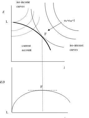
The bold current account constraint in Figure 1 shows all combinations of i
and E that give a balance on the current account. The iso-interest curves give all combinations of i and E that leave the foreign investor indifferent – they give the same flow of interest income measured in foreign currency – and the iso-income curves give all combinations of i and E that leave the home country as well off in terms of national income net of interest payments measured in foreign currency. At
F, the interest income of foreign investors measured in foreign currency is maximized, while the home country is best off at point L, where the interest rate is equal to zero and the currency is strengthened to generate a current account balance. Local authorities would never decide to pay interest to foreigners in the absence of leakages – to move from point L toward F. We now turn to studying the effect of leakages on this decision.
3.2
Leakages introduced
Leakages involve exporters, who have revenues in foreign currencies, buying domestic currency offshore. This transaction involves the exporters depositing foreign currency into bank accounts in foreign banks and getting a deposit in local currency in an Icelandic bank using the offshore exchange rate in the transaction. The exporters face the possibility of fines and even criminal prosecution if the trade is discovered by the authorities.
Cumby and Levich (1987) survey and analyze the various definitions and measures of capital flight and distinguish this concept from ordinary capital flows. The definition that fits our purposes is that capital flights entail a difference between what is privately and socially optimal. In particular, the decision to evade capital controls may be beneficial for an investor but may reduce domestic social welfare by destabilizing financial market, raising a country’s borrowing needs and
_________________________
20 The iso-income curves are convex because .
Figure 1. Foreign investors’ interest income, without leakages
The bold current account constraint shows all of the combinations of i and E that give a balance on the current account. The iso-interest curves give all combinations of i and E that leave the foreign investor indifferent – they give the same flow of interest income measured in foreign currency – and the iso-income curves give all combinations of i and E that leave the home country as well off in terms of national income net of interest payments measured in foreign currency.
i
E
eX+eM=1
iED
L
F
F
i
iso-interest curves iso-income
curves
current account
lowering domestic investment. Moreover, the depreciation of the exchange rate affects other individuals, in particular the many unhedged borrowers who had borrowed in foreign currencies. 21
The usefulness of capital controls depends on how successful they are at preventing owners of domestic currency from being able to sell the currency offshore to exporters that need to buy local currency using their foreign currency earnings. In order to analyze the effect of interest rate changes on the exchange rate, one must therefore study the effect of changing the interest rate on the decisions made by both owners of domestic currency and exporters of goods and services.
In this section, we describe the behavior of exporters that must decide whether to buy domestic currency onshore or offshore – in the latter case, risking detection and penalties. We then turn to the decision of the owners of domestic currency assets, who must decide whether to invest in domestic currency assets or buy foreign currency from the exporters offshore, then invest in foreign bonds and subsequently return to the domestic currency using the onshore currency market. We start by describing exporting firms’ decision about where to buy domestic currency, thereby describing the demand for the domestic currency in the offshore market as well. Allowing for leakages, the flow of export revenues into the onshore foreign exchange market depends on the difference between the onshore and offshore exchange rates, E and e. The typical exporting firm maximizes its domestic currency profits, defined as the sum of domestic currency revenue onshore and offshore net of the expected cost of being caught evading the capital controls. The expected costs of evasion depends on the volume of offshore trading,
�0(� − ��) +�1(� − ��)2, where XL is the volume of exports appearing in the
onshore export market and �0> 0 and �1> 0. The expected profits in units of output are given by equation (8),
_________________________
, (8)
where e is the offshore exchange rate and E the onshore exchange rate, as before. The volume XL that shows up in the onshore market generates less revenue – in terms of domestic currency – than that which shows up in the offshore market. Each unit of exports generates e units of foreign currency in the offshore market – this is the market exchange rate – but when this is brought back in using the onshore market at a higher exchange rate, the revenue coming from exports through the onshore market measured in domestic currency is lower per unit of output sold than that coming from the offshore market because e<E. It follows that exporting firms will lose from buying the domestic currency onshore, where it is more expensive. However, buying onshore will reduce the expected cost of detection.
The first-order condition with respect to XL gives exports traded in the offshore market as a positive function of the difference between the onshore and offshore exchange rates and a negative function of the intensity of capital controls monitoring, t0:22
. (9)
The onshore exchange rate is determined so as to generate a balanced current account, taking only into account the part of exports that show up onshore XL, which, from equations (2) and (9), gives:
, (10)
or, using (9):
(11)
A larger exchange rate differential – making the currency relatively more expensive onshore – will increase leakages and lower XL, while an increase in
monitoring t0and t1will raise X L
by increasing the likelihood that violations of the capital controls will be detected. Greater enforcement of the controls will strengthen the currency, while an offshore depreciation will weaken it by encouraging local exporters to buy domestic currency offshore.
We turn next to the decision faced by holders of domestic currency: whether to buy bonds denominated in the domestic currency or, alternatively, to leave the domestic currency through the offshore market, invest in foreign bonds, and then return to the domestic currency through the onshore market (where the value of the domestic currency is higher). This describes the supply of domestic currency in the offshore market. In equilibrium, the expected return from remaining in the domestic currency is equal to the expected return from leaving through the offshore market. The equilibrium condition gives a relationship between domestic interest rates, foreign interest rates, the expected onshore exchange rate, and the offshore exchange rate. The following equation states the equilibrium condition by setting the return on remaining in the domestic currency asset earning an interest rate i equal to the return on exiting the currency offshore and investing in foreign assets that yield an interest rate of i* plus a risk premium on domestic currency assets p:
�� =��∗− ���(��+1� ) +���(��) +�� (12)
This interest parity condition determines the offshore exchange rate given the domestic and foreign interest rate, the expected onshore exchange rate, and the risk premium. An increase in domestic interest rates will raise the expected return from holding domestic currency assets, and this will make the offshore exchange rate rise – because of a smaller supply of domestic currency in the offshore market – until the expected return from exiting the currency offshore is raised to equal the higher domestic currency interest rates. An increase in the foreign interest rate i*
will have the opposite effect of making the offshore exchange rate fall by increasing the supply of domestic currency in the offshore market in order to reduce the return on exiting the currency back to the previous level. An increase in the risk premium p will lower the offshore exchange rate for the same reason, and finally, the higher the expected future onshore exchange rate , the higher the offshore exchange rate.
Together, equations (9), (11), and (12) determine the onshore exchange rate E, the offshore rate e, and the volume of exports that show up in the onshore market
1
e t
XL. The equations reveal that cutting interest rates has both a flow effect – captured by equation (11) – and a stock effect – captured by equation (12). Lower interest rates strengthen the currency by reducing the required trade balance. This is the flow effect, which is essentially the transfer problem discussed by Keynes (1929). But they also lower the expected return from holding domestic currency assets, which makes the offshore exchange rate fall when leakages increase, which then lowers the volume of exports that go to the onshore market XL, thereby making the onshore exchange rate fall. This is the stock effect.
Substituting equation (12) into equation (11) gives
(13)
Taking the total differential of the equation gives the effect of changing domestic interest rates on the onshore exchange rate:
, (14)
where Ω=��+���−1 2⁄ �1− ��− ��< 0 according to equation (4). The effect of changing the domestic interest rate therefore depends on the level of debt and the penalty imposed on those exporters who violate capital controls by buying domestic currency offshore. Once debt exceeds a threshold, which is lower the larger is the penalty for violating the capital controls (t1), the flow effect of higher
interest rates dominates the stock effect and higher interest rates will only make the currency depreciate because of an increase in the trade surplus required to finance the interest payments. The threshold is given by the term 1/(2t1), so that the lower the value of t1 in equation (8), the higher the level of the threshold. This implies that with a low level of t1, when the capital controls are not rigorously enforced so that buying domestic currency offshore is not as costly in terms of penalties, a higher interest rate is more likely to help boost the exchange rate. In contrast, high interest rates are most likely to lower the exchange rate when the level of debt D is high and the capital controls are enforced with vigor; i.e., t1 is high. Coming back to Figure 2 above, with low levels of debt the current account
constraint may be upward-sloping, but with high levels of debt it remains downward-sloping and the optimal rate of interest for the home country remains equal to zero.
In contrast to the effect of raising domestic interest rates, the effects of higher foreign interest rates, a higher expected onshore exchange rate, a higher country risk premium, and a higher cost t0 of evading capital controls do not depend on the
level of debt. Again, taking the total differential of equation (13) above shows that an increase in the foreign interest rate i* makes the onshore exchange rate fall, as does an increase in the country risk premium p. In both cases, there is an incentive for owners of domestic currency assets to leave the domestic currency offshore, invest in foreign bonds, and then re-enter onshore. The effect is to make the offshore exchange rate fall, making exporters buy local currency offshore and therefore lowering the onshore exchange rate. In contrast, an increase in the expected onshore exchange rate and the penalty from evading controls t0 will raise
the onshore exchange rate by increasing the cost to exporters of using the offshore market and reducing the expected profits to investors of leaving the currency for foreign bonds. The derivatives are shown in Appendix I.
We note that the capital controls were the result of financial circumstances that affect the exchange rate through channels that have nothing to do with the interest rate since, in their extreme form, financial crises lead to panic and erratic behavior. We account for these other factors by including the risk premium measured by the CDS on Icelandic government bonds, as any panic affecting the currency would show up in the CDS market.
From the theoretical framework presented here, we can argue that raising domestic interest rates may or may not have the effect of raising the exchange rate, all depending on the level of debt in the form of domestic assets held by foreign investors. When the level of domestic assets owned by foreign investors is high and the capital controls are stringently monitored, an increase in domestic interest rates will make the exchange rate fall because of the greater outflows of interest payments to foreign investors that require a larger trade surplus. But note that the effect is symmetric – it does not matter whether interest rates are raised or lowered – and linear.23 In contrast, a fall in foreign interest rates does help the home
_________________________
country because it reduces leakages so that the offshore exchange rate rises, making it less tempting for exporters to sell their foreign currency offshore. Similarly, a fall in the risk premium on domestic currency assets would have the effect of raising the onshore exchange rate through reduced leakages, and the same applies to expectations of a higher future onshore exchange rate.
4
Empirical study
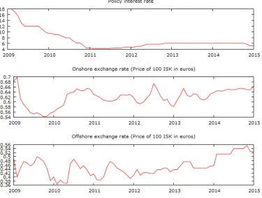
The Central Bank of Iceland began monetary easing in March 2009, which was justified by rapidly declining inflation. It reduced its policy rate by 1% (from 18% to 17%) in March, then by 1.5% (to 15.5%) in April, and finally, to 13% in May. Three more cuts followed in 2009, lowering the rate to 10% by the end of the year. Further cuts followed in 2010, lowering the policy rate to 4.25% by the beginning of 2011. Figure 2 shows the policy rate, the onshore exchange rate, and the offshore exchange rate between January 2009 and March 2015. Note that the EURISK exchange rate is fairly stable at around 0.62 euros per 100 ISK, while the offshore rate fluctuates around 0.46 euros per 100 ISK.
One pattern that is visible in Figure 2 is the lax monitoring of the capital controls in 2009, which makes the onshore rate fall and the offshore rate rise. In November 2009, enforcement of the capital controls was tightened, subsequently making the onshore rate rise and the offshore rate fall. Increased leakages appear also to have occurred in 2011.
The pattern of changes in the policy rate, the onshore exchange rate, and the offshore exchange rate can be used to discriminate between the different channels from interest rates to exchange rates, discussed in Section 3 above. We employ a simple VECM based on the interest parity condition in equation (12). For our experiment, we use the policy rates of the Central Bank of Iceland and the ECB for
� and �∗ respectively, after subtracting the corresponding CDS spread to correct for the risk premium. For the estimation of the model, we use monthly data from January 2009 to February 2015.
Figure 2. Interest rates and exchange rate
risk, this is not a realistic assumption. We have already corrected for the risk premium, but the issue of transaction costs remains.24 Regardless, the condition can serve as an equilibrium benchmark in the VECM, from which the economy deviates in the short run.
Rewriting equation (12) and making the strong assumption of rational expectations yields:
log(��+1)−log(��) =��∗− ��+εt (15) _________________________
where εt is a white noise term. A p-th order VECM in the variables in (15), taking the eurozone interest rate to be exogenous, is:
∆��=�0+���−1+∑��=1��Δ��−�+�� (16)
where ��′ = (log(��) , log(��) ,��), �′� = (log(��) , log(��) ,��,��∗), � is a parameter matrix with rank equal to the number of cointegrating relations, �0,...,�� are matrices of parameters, and �� a vector of error terms.
Performing unit-root tests on the four variables suggests that all of them are non-stationary, although the Augmented Dickey–Fuller and Kwiatkowski– Phillips–Schmidt–Shin tests do not agree in the case of log(�). See Tables A2.1 and A2.2 in Appendix 2. The differences of all variables are stationary, so we conclude that that they are I(1). Allowing a maximum of 12 lags, the Akaike and Hannan-Quinn Information Criteria suggest 12 lags, while the Bayesian Information Criterion suggests 1 (Table A2.3). As the suggestions of the criteria differ significantly, we resort to residual diagnostics. In both cases, the null of normality is rejected, but there is less evidence of autocorrelation in the residuals with 12 lags, so we opt for a VECM(11).
A Johansen cointegration, shown in table A2.5 in Appendix 2, test suggests that there exist two cointegrating relations between the variables. For the cointegrating relationships to be identified, we must impose at least one linear restriction on each vector. In the first we set the coefficient of the policy instrument to negative one and the coefficient on the offshore rate to 0. This is justified by the observation that in setting interest rates the stated goal of the central bank was to stabilize the exchange rate, taking into account the difference between domestic and foreign interest rates. In the second, we set the foreign interest rate coefficient to zero and the onshore coefficient to negative 1. Here the onshore rate is determined by the domestic interest rate and the offshore exchange rate. The results show that in the long run the domestic interest rate is a positive function of the onshore rate and the foreign interest rate. The second relationship shows that the onshore exchange rate is a positive function of the offshore exchange rate and the policy instrument.
exchange rates are significant, but none of the policy rate lags are. Both error correction terms are significant in the onshore equation, the first in the policy rate equation, and the second in the offshore equation.
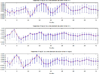
Our Cholesky ordering identification strategy is to order the policy instrument first, so that it responds to the two exchange rates with a lag. The second term is the offshore exchange rate, which responds to the onshore rate with a lag.25 The impulse response functions are shown in Figures 3 and 4 below, in response to a one standard deviation shock with 90% boot strap confidence intervals.
The impulse response function of the onshore exchange rate in response to a shock to domestic interest rates is shown in the top panel of Figure 3. Note that the effect is not statistically significant from zero for most of the months following the shock. The impact response at time zero can be compared to the one for the period before capital controls, as shown in Appendix 3, when the response appears to have been stronger in the very short run. We conclude that changes in the interest rate have a very weak effect on the onshore exchange rate in a capital control regime.
The impulse response function for the offshore exchange rate in response to a shock to domestic interest rates is shown in the middle panel. The offshore rate appreciates initially, which in terms of our model is due to a reduced supply of the domestic currency in the offshore market. The effect is significant for the first four months following the shock, as indicated by the confidence intervals.
The bottom panel shows the response of the onshore exchange rate to a shock to the offshore exchange rate. A rise in the offshore rate yields a rise in the onshore rate, although the effect is only positively significant at the four and five month mark and then between 12 and 15 months. This occurs in our model when it becomes more profitable to convert export earnings into the local currency onshore.
_________________________
Figure 3. Impulse responses following an interest rate and offshore exchange rate shock
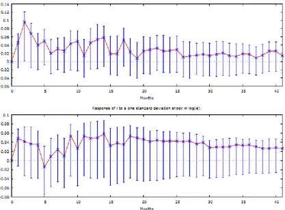
Figure 4. Impulse responses following an exchange rate shock
monetary policy responded to exchange rate movements and interest rate increases had the short-term effect of raising the exchange rate while in the capital control period the central bank did not respond in the same way to exchange rate movements nor did interest rate changes have as strong an effect on the exchange rate. The lower panel of the figure has the effect of a shock in the offshore rate on the interest rate, but the effect is not statistically significant from zero.
exchange rate initially explain the majority of the variance in the offshore exchange rate, but at around the two-year mark the interest rate explains roughly 60 percent and the onshore rate 10 percent. Shocks to the onshore exchange rate explain around 95 percent of the variance in the onshore rate initially, but in three years interest rates explain around 50 percent and the offshore rate 20 percent.
5
Conclusions
This paper has derived a relationship between central bank interest rates and exchange rates under a capital control regime. The onshore and offshore exchange rates are determined by the requirement of a balance on the current account and an interest parity condition.
Higher interest rates onshore may raise both onshore and offshore exchange rates by inducing owners of local currency assets not to sell local currency offshore. This will make the offshore exchange rate rise, thereby discouraging exporters from buying local currency offshore and increasing the supply of foreign currency onshore. The onshore exchange rate will increase as a result. There is also an effect that goes in the opposite direction: Higher interest rates increase the flow of interest income to foreigners through the current account, making the onshore exchange rate fall, which then makes exporters turn to the onshore market, lowering the offshore rate. The former effect is likely to dominate when the level of debt held by foreigners is low and the enforcement of capital controls weak while the latter effect dominates when the level of debt is high and capital controls are strongly enforced.
a fall in leakages. An offshore rise in the exchange rate causes the onshore exchange rate to rise, which in our model occurs when exporters turn to the onshore market because of the offshore appreciation, although this effect is weak.
While the effects of changes in interest rates are statistically weak, the paths of exchange rates indicate a strong effect of the enforcement of the capital controls. Better enforcement increased the difference between the onshore and the offshore exchange rate in late 2009 and 2010, raising the onshore rate and weakening the offshore rate.
Overall, the experience suggests a very weak effect of interest rates on the onshore exchange rate. It follows that cutting interest rates from a very high level is not likely to make a currency depreciate in an effective capital control regime, highlighting the importance of the effective enforcement of the controls.
References
Agnieszka, S. (2008). International parity relations between Poland and Germany: A cointegrated VAR approach. MPRA Paper 24057.
https://mpra.ub.uni-muenchen.de/24057/
Agosin, M.R., and F. Huaita (2012). Overreaction in capital flows to emerging markets: Booms and sudden stops. Journal of International Money and Finance 3: 1140–1155.
http://www.sciencedirect.com/science/article/pii/S0261560611002002
Ariyoshi, A., Habermeier, K., Laurens, B., Otker-Robe, I., Canales-Kriijenki, J.I., and A. Kirilenko (2000). Capital controls: Country experiences with their use and liberalization. IMF Occasional Paper 190.
http://www.imf.org/external/pubs/ft/op/op190/
Bacchetta, P., and K. Behima (2010). The demand for liquid assets in international capital flows. Unpublished mimeo.
Benediktsdottir, S., Danielsson, J., and G. Zoega (2011). Lessons from a collapse of a financial system. Economic Policy 26 (66): 183–235.
http://econpapers.repec.org/article/blaecpoli/v_3a26_3ay_3a2011_3ai_3a66_3ap_3a1 83-231.htm
Bordo, M.D. (2008). Growing up to financial stability. Economics: The Open-Access, Open-Assessment E-Journal, 2 (2008–12): 1–17.
http://dx.doi.org/10.5018/economics-ejournal.ja.2008-12
Broner, F., Didier, T. Erce, A., and S. Schmukler (2010). Financial crises and international portfolio dynamics. Mimeo.
http://m.repositori.upf.edu/bitstream/handle/10230/6358/1227.pdf?sequence=1
Caballero, R. Farhi, E., and P.-O. Gourinchas (2008). An equilibrium model of “global imbalances” and low interest rates. The American Economic Review 98 (1): 358–393.
https://www.aeaweb.org/articles?id=10.1257/aer.98.1.358
Calvo, G., Leiderman, L., and C. Reinhart (1993). Capital inflows and real exchange rate appreciation in Latin America: The role of external factors. IMF Staff Papers 40 (1): 108–151. http://www.jstor.org/stable/3867379
Calvo, G., Leiderman, L., and C. Reinhart (1996). Inflows of capital to developing countries in the 1990s. The Journal of Economic Perspectives 10 (2): 123–139.
https://www.aeaweb.org/articles?id=10.1257/jep.10.2.123
Caporale, G.M., Cipollini, A., and P.O. Demetriades (2005). Monetary policy and the exchange rate during the Asian crisis: Identification through heteroscedasticity.
Journal of International Money and Finance 24: 39–53.
http://www.sciencedirect.com/science/article/pii/S0261560604000920
Chinn, M.D., and S.J. Wei (2013). A faith-based initiative meets the evidence: Does a flexible exchange rate regime really facilitate current account adjustment? Review of Economics and Statistics 95 (1): 168–184.
http://www.mitpressjournals.org/doi/abs/10.1162/REST_a_00244?journalCode=rest
Chuhan, P. Claessens, S., and N. Mamingi (1998). Equity and bond flows to Latin America and Asia: The role of global and country factors. Journal of Development Economics
55 (2): 439–463.
http://www.sciencedirect.com/science/article/pii/S0304387898000443
Cumby, R., and R. Levich (1987). On the Definition and Magnitude of Recent Capital Flight, in: D. Lessard and J. Williamson (Eds.), Capital Flight and Third World Debt. Washington, DC: Institute for International Economics.
Danielsson, J., and G. Zoega (2009). The collapse of a country (second edition).
www.RiskResearch.org. http://www.riskresearch.org/files/DanielssonZoega2009.pdf Diamond, D.W., and P.H. Dybvig (1983). Bank runs, deposit insurance and liquidity.
Journal of Political Economy 91 (3): 401–419.
Escudé, G. J. (2014). The possible trinity: Optimal interest rate, exchange rate, and taxes on capital flows in a DSGE model for a small open economy. Economics: The Open-Access, Open-Assessment E-Journal, 8 (2014–25): 1–58.
http://dx.doi.org/10.5018/economics-ejournal.ja.2014-25
Fernandez-Arias, E. (1996). The new wave of private capital inflows: Push or pull?
Journal of Development Economics 48 (2): 389–418.
http://www.sciencedirect.com/science/article/pii/0304387895000410
Flood, R.P. and O. Jeanne (2001). An interest rate defense of a fixed exchange rate?
Journal of International Economics 66: 471–484.
http://www.sciencedirect.com/science/article/pii/S0022199604001230
Forbes, K.J. (2016). Capital controls. In Banking Crises (pp. 39–43). Palgrave Macmillan UK.
Forbes, K. J., and F. E. Warnock (2012). Capital flow waves: Surges, stops, flight, and retrenchment. Journal of International Economics 88 (2): 235–251.
http://www.sciencedirect.com/science/article/pii/S0022199612000566
Fratzscher, M. (2012). Capital flows, push versus pull factors and the global financial crisis. Journal of International Economics 88: 341–356.
Goldfajn, I., and P. Gupta (2003). Does monetary policy stabilize the exchange rate following a currency crisis? IMF Staff Papers 50 (1): 90–114.
http://www.jstor.org/stable/4149949
Gosh, A.R., Chamon, M., Crowe, C., Kim, J.I., and J. D. Ostry (2009). Coping with the crisis: Policy options for emerging market countries. IMF Staff Position Note 23, SPN/09/08. https://www.imf.org/external/pubs/ft/spn/2009/spn0908.pdf
Gudmundsson, G.S., and G. Zoega (2014). Age structure and the current account.
Economics Letters 123 (2): 183–186.
http://www.sciencedirect.com/science/article/pii/S0165176514000573
Ju, J., and S.-J. Wei (2011). When is quality of financial system a source of comparative advantage? Journal of International Economics 84 (2): 178–187.
http://www.sciencedirect.com/science/article/pii/S0022199611000304
Kaplan, E., and D. Rodrik (2001). Did the Malaysian capital controls work? NBER Working Paper 8142. http://www.nber.org/papers/w8142
Katsmini, M., and G. Zoega (2016). European integration and the Feldstein-Horioka Puzzle. Oxford Bulletin of Economics and Statistics, forthcoming.
http://dx.doi.org/10.1111/obes.12130
Keynes, J.M. (1929). The German transfer problem. The Economic Journal 39 (153): 1–7.
http://www.jstor.org/stable/2224211
Lacerda, M., Fedderke, J.W., and L.M. Haines (2010). Testing for purchasing power parity and uncovered interest parity in the presence of monetary and exchange rate regime shifts. South African Journal of Economics 78 (4): 363–382.
http://onlinelibrary.wiley.com/doi/10.1111/j.1813-6982.2010.01254.x/abstract Lane, P.R., and G.M. Milesi-Ferretti (2012). External adjustment and the global crisis.
Journal of International Economics 88 (2): 252–265.
http://www.sciencedirect.com/science/article/pii/S0022199611001772
Martin, F.E. (2016). Exchange rate regimes and current account adjustment: An empirical investigation. Journal of international Money and Finance 65: 69–93.
http://www.sciencedirect.com/science/article/pii/S0261560616300171
Mendoza, E., Quadrini, V., and J.V. Rios-Rull (2009). Financial integration, financial development and global imbalances. Journal of Political Economy 117 (3): 371–416.
http://www.journals.uchicago.edu/doi/10.1086/599706
Milesi-Ferretti, G.M., and C. Tille (2011). The great retrenchment: International capital flows during the global financial crisis. Economic Policy 26: 289–346.
Ndikumana, L., and J.K. Boyce (2010). Measurement of Capital Flight: Methodology and Results for Sub-Saharan African Countries. African Development Review 22(4): 471– 481. http://onlinelibrary.wiley.com/doi/10.1111/j.1467-8268.2010.00243.x/abstract Reinhart, C.M., and K.S. Rogoff, (2009). The aftermath of financial crises. American
Economic Review 99(2): 466–472.
https://www.aeaweb.org/articles?id=10.1257/aer.99.2.466
Appendix 1
Taking the total derivative of the following equation
gives the derivatives of the onshore exchange rate with respect to debt, the risk premium and the foreign rate of interest. We start with debt;
�� ��=
�� ٠< 0
where Ω=��+���−1 2⁄ �1− ��− ��< 0 according to equation (4). Thus a higher level of debt reduces the equilibrium exchange rate in order to make possible the transfer of interest payments to foreign investors.
The effect of a higher foreign rate of interest goes in the same direction:
�� ��∗=
�
2�1Ω< 0
A higher foreign rate of interest has the effect of making it more profitable to sell domestic currency offshore to exporters who then reduce the supply of foreign currency in the onshore market reducing the onshore exchange rate.
A higher risk premium also has the effect of reducing the onshore exchange rate for the same reason as an increase in the foreign rate of interest:
Finally,
�� ��0=−
�
2�1Ω> 0
Thus better monitoring of the capital controls will raise the onshore exchange rate by making it more costly for exporters to evade controls.
Appendix 2
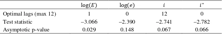
The results of the ADF tests, where the null hypothesis is that the process contains a unit root (see Table A2.1).
TableA2.1. Augmented Dickey–Fuller Test Results
log(�) log(�) � �∗
Optimal lags (max 12) 1 0 12 0
Test statistic –3.066 –2.390 –2.741 –2.782 Asymptotic p-value 0.029 0.148 0.067 0.066
The results of the KPSS tests with lag truncation parameter equal to 3, where the null hypothesis is of stationarity (see Table A2.2.).
Table A2.2. Kwiatkowski–Phillips–Schmidt–Shin Test Results
log(�) log(�) � �∗
Test statistic 0.691 0.841 0.500 1.614 Interpolated p-value 0.016 < 0.01 0.044 < 0.01
The critical values for the KPSS test are: 10% – 0.350, 5% – 0.462 and 1% – 0.731.
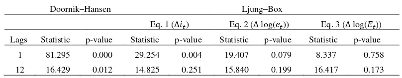
The null of the DH test is one of multivariate normality. The null of the LB test is that there is no autocorrelation up to the 12th order.
The Johansen cointegration tests results are shown in Table A2.3.
Table A2.3. VAR lag selection criteria
Lags Log-likelihood AIC BIC HQC
1 212.717 –6.378 –5.863 –6.176 2 226.042 –6.517 –5.694 –6.194 3 226.966 –6.257 –5.125 –5.812 4 235.935 –6.256 –4.815 –5.690 5 253.141 –6.521 –4.771 –5.834 6 266.529 –6.662 –4.604 –5.854 7 273.986 –6.612 –4.245 –5.683 8 289.202 –6.813 –4.137 –5.762 9 301.461 –6.918 –3.933 –5.746 10 315.985 –7.096 –3.803 –5.803 11 330.396 –7.271 –3.668 –5.856 12 360.720 –7.959 –4.048 –6.423
Table A2.4. Residual diagnostics
Doornik–Hansen Ljung–Box
Eq. 1 (∆��) Eq. 2 (∆ log(��)) Eq. 3 (∆ log(��)) Lags Statistic p-value Statistic p-value Statistic p-value Statistic p-value 1 81.295 0.000 29.254 0.004 19.407 0.079 8.337 0.758 12 16.429 0.012 14.825 0.251 15.840 0.199 16.417 0.173
Table A2.5. Johansen Trace and Max Test Results
Rank, � Eigenvalue Trace test p-value Max test p-value
0 0.646 97.534 0.000 64.305 0.000
1 0.407 33.229 0.000 32.398 0.000
The null of the trace test is that there are r or fewer cointegrating vectors. The null hypothesis of the max test is that the number of cointegrating vectors is equal to r.
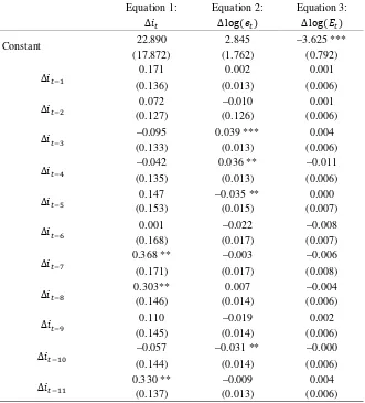
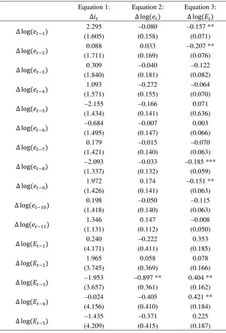
Finally, the results of estimating the VECM are shown in Table A2.6.
Table A2.6. Estimation results for VECM(11) for the period 2009–2015
Equation 1:
Adjustment term 2 –0.220 (3.345)
Maximum likelihood estimates, observations 2010:01–2015:02 (T = 62).
*** denotes significance at the 1% level. ** denotes significance at the 5% level.
Appendix 3
∆log(��+1) =��∗− ��+εt (A3.1) Unit root tests suggest that all variables are no greater than I(1). A Johansen test suggests one cointegrating vector. The HQC and BIC suggest 2 and 1 lags respectively, while the AIC suggests 11. Residual diagnostics favour the more parsimonious specifications. The results of estimating a VECM(2) are as shown in Tablbe A3.1.
For impulse responses and variance decomposition, we order interest rates first. All impulse responses are in response to a shock of one standard deviation and are shown with 90% boot strap confidence intervals. The impulse response functions are as follows:
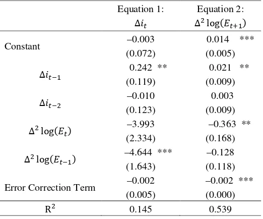
Table A3.1. Estimation results for VECM(2) for the period 2000–2008
Equation 1:
∆��
Equation 2:
∆2log(� �+1)
Constant –0.003 (0.072)
0.014 *** (0.005)
∆��−1 0.242 ** (0.119) 0.021 ** (0.009)
∆��−2 (0.123) –0.010 0.003 (0.009)
∆2log(�
�) (2.334) –3.993 –0.363 ** (0.168)
∆2log(�
�−1) –4.644 *** (1.643) (0.118) –0.128
Error Correction Term –0.002 (0.005)
–0.002 *** (0.000)
R2 0.145 0.539
Maximum likelihood estimates, observations 2000:05–2008:12 (T =104).
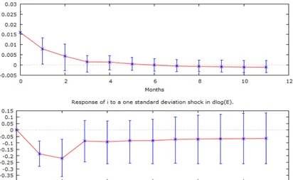
Figure A3.1. Impulse responses.
The top panel of Figure A3.1 shows the impulse response of the difference in the exchange rate to a shock in policy rates. The difference is positive and statistically significant for the first period, but insignificant from zero thereafter. The lower panel of Figure A3.1 shows that an increase in the exchange rate is met with a statistically significant decline in the policy rate for the first two periods, but insignificant after the second period.
Figure A3.2. Variance decomposition for the policy interest rate.
Appendix 4
The following three figures show the variance decomposition forecast of the three variables in the VECM(11):
Figure A4.1. Variance decomposition for the policy interest rate.
Please note:
You are most sincerely encouraged to participate in the open assessment of this article. You can do so by either recommending the article or by posting your comments.
Please go to:
http://dx.doi.org/10.5018/economics-ejournal.ja.2016-17
The Editor