Published by Canadian Center of Science and Education
The Local Characteristics of Indonesian Seas and Its Possible
Connection with ENSO and IOD: Ten Years Analysis of Satellite
Remote Sensing Data
I Dewa Nyoman Nurweda Putra1,2 & Tasuku Tanaka1 1
Graduate School of Science and Engineering, University of Yamaguchi, Yamaguchi Ken, Ube Shi Tokiwadai, Japan
2
University of Udayana, Bali, Indonesia
Correspondence: I Dewa Nyoman Nurweda Putra, Graduate School of Science and Engineering, University of Yamaguchi, 755-8611 Yamaguchi Ken, Ube Shi Tokiwadai 2-16-1, Japan. Tel: 81-836-859-129; Center for Remote Sensing and Ocean Science (CReSOS), University of Udayana, PB Sudirman Street, Denpasar 80232, Bali, Indonesia. Tel: 62-361-256-162. E-mail: [email protected]
Received: April 26, 2013 Accepted: May 23, 2013 Online Published: June 24, 2013
doi: 10.5539/esr.v2n2p153 URL: http://dx.doi.org/10.5539/esr.v2n2p153
Abstract
The overall objective of this study is to investigate the local characteristics of the Indonesian Seas in response to the 6 months, seasonal and inter-annual variations. A moving averages method with 3, 6 and 12 months of lengths has been used to show the temporal variability. Using satellite observed datasets for the 10 year period from December 1999-November 2009, the results of moving averages indicate the 6 months and seasonal variabilities of sea surface temperature (SST), zonal-component of wind speed (U-WS) and rain rate (RR) in most of the Indonesian Seas area. It is also interesting to note that, although in the same latitude with the strong seasonal variability area, a stable condition of SST occurs in some particular areas. The cross-lag correlation analysis shows the relationship among indices with several month time lags. After removing the seasonal variability, the possible connection of indices with the El Nino-Southern Oscillation (ENSO) and the Indian Ocean Dipole (IOD) phenomena in the Indonesian Seas can be detected by the 6 month moving averages method.
Keywords: Indonesian Seas, seasonal variability, 6-months variability, moving averages, ENSO, IOD 1. Introduction
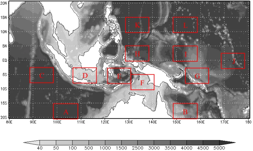
The Indonesian Seas, a semi-closed marginal sea, separates the Pacific Ocean from the Indian Ocean (see Figure 1) with a chain of big and small islands. The bathymetry is generally shallow (<100 m) throughout the western area of the inner Indonesian Seas, while the abyssal sea basin in the east of the inner Indonesian Seas has the depths of 5000 m. The Indonesian Seas lie on and near the Equator including “warm pool” with its high temperature. The region also has an important pathway for water transport (Gordon et al., 2003, 2010; Sprintall et al., 2004; Gordon, 2005), the Indonesian throughflow (ITF). ITF affects both the regional circulation and thermal structure (Godfrey 1996; England & Huang, 2005).
characters for the local areas in the Indonesian Seas. Then, we compare those temporal variabilities with the ENSO and IOD indices to consider their influence to the Indonesian Seas. We also show the locality of those variabilities and the correlation of indices.
Figure 1. The bottom topography map (scale in meter) of the Indonesian Seas derived from ETOPO 2 minutes (Smith and Sandwell 1997).
Axes indicate longitude 80˚ - 180˚ E and latitude 20˚ S - 20˚ N. Areas with deep water are shaded in light grey, areas with shallow water are shaded in dark grey and areas with no available data are in white
2. Methodof Analysis
We reveal the ocean characteristics from the monthly SST, U-WS and RR in 10 years (December 1999 – November 2009) by satellites observation. Those three data show the clear cyclic variability of the ocean characteristics (Swardika et al., 2012; Nurweda & Tanaka, 2012).
To determine the local variability, we calculate the average of the indices over each local area from the monthly grid data, which is downloaded from the satellite data archives. In order to analyse the temporal variability of indices in the Indonesian Seas, we need to take account of the 6 months variability because the solar looking angle becomes at zenith twice a year.
To detect the seasonal variability, we calculate the 6 months moving averages in which no 6 months variability appears. If there exists a longer than 12 months cyclic variability, it appears in the 12 months moving averages. We should know whether those longer cyclic variabilities exist. Thus we calculate the 6 and 12 months moving averages.
To detect the 6 months variability, we calculate the 3 months moving averages. If a seasonal variability exists, it also appears in the 6 months moving averages. But we can distinguish the 6 months variability from the seasonal variability by carefully expecting the average.
The moving averages for the month-i are calculated as follows:
where xi is the original monthly data and Xi is the monthly data of the moving averages. The value of Xi
corresponds to the middle of the month.
The ENSO index is defined with the 3 months moving averages of SST in the central tropical Pacific Ocean. If we compare the indices in the Indonesian Seas with the ENSO index, we should take account of both 6 months and seasonal variabilities. As we will show later, all the indices in the ENSO Index area have neither 6 months nor seasonal variabilities. For the comparison, we need the indices free from the 6 months and seasonal variabilities. Thus, the connections of indices with the ENSO signal are observed by the 6 months moving averages of the deseasonalized indices. The deseasonalized (di) indices can be calculated as follows:
; , , , … , (3)
where:
(4)
Wiis the monthly data with no temporal variability longer than 12 months; xi is the original monthly data and Xi is
calculated by the Equation 1 with k = 6.
We also calculate the auto-correlation of SST, U-WS and RR in order to analyse the temporal variability of indices. The auto-correlation function (Rxx) is expressed as follows:
(8)
To identify the relationship among the indices, the cross-correlation is calculated. The cross-correlation (Rxy) is
expressed as follows:
∑ ∑ (14)
σ x ̅ σ (15)
̅ ∑ ∑ (16)
3. Dataset
We use the monthly data of SST and U-WS that are compiled by the Remote Sensing Systems (REMSS) from TRMM-TMI and QuikSCAT dataset in the 0.25˚ × 0.25˚ grid (ftp://ftp.remss.com). The physical dimension of SST and UWS are [deg. Celsius] and [m/s], respectively. For precipitation, we use the TRMM combined level 3 (3B43) versions 6 data, which is compiled and supplied by the Earth Observation Research Center, Japan Aerospace Exploration Agency (JAXA EORC). The 3B43 version 6 data is recorded monthly in 0.25˚ grid of horizontal resolution, and its physical dimension is [mm/month].
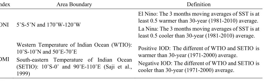
For the ENSO and IOD phenomena, the Ocean Nino Index (ONI) and Dipole Mode Index (DMI) are used (see Table 1 for the complete definition of the indices). The time series dataset of indices are prepared by National Oceanic and Atmospheric Administration (NOAA) - Climate Prediction Center (CPC) for the ONI dataset and the Japan Agency for Marine-Earth Science and Technology (JAMSTEC) for the DMI dataset.
Table 1. Specifications of the SST anomaly index
Index Area Boundary Definition
ONI 5˚S-5˚N and 170˚W-120˚W
El Nino: The 3 months moving averages of SST is at least 0.5 warmer than 30-year (1981-2010) average. La Nina: The 3 months moving averages of SST is at least 0.5 cooler than 30-year (1981-2010) average.
DMI
Positive IOD: The different of WTIO and SETIO is warmer than 30-year (1971-2000) average.
Negative IOD: The different of WTIO and SETIO is cooler than 30-year (1971-2000) average.
We analyse the whole Indonesian Seas, from 80˚ - 180˚ E in longitude and from 20˚ S - 20˚ N in latitude (see Figure 1), which spans the tropics of both Indian and Pacific Oceans. In order to analyze the local characteristics, the Indonesian Seas is divided into three regions with twelve areas. These three regions represent the south subtropical region, the near-equatorial region and the north subtropical region. The twelve local areas are (see Figure 1): area A covers the southeast Indian Ocean (100˚ E - 110˚ E, 20˚ S - 15˚ S); area B covers the southwest
The 3, 6 and 12 months moving averages for all areas are shown in Figures 2 to 13. The summaries of the seasonal and 6 months variabilities are presented in Tables 2 and 3, respectively. The auto-correlation of indices is presented in Table 4. The correlation coefficients and time lag among indices are presented in Table 5.
22). Thus, in this paper the abnormal year of IOD is considered only for the year of 2007.
From the all 12 months averages, we observed that there is no longer than 12 months variability, or more precisely, the cyclic variability of longer than 12 months in the Indonesian Seas.
4.1 The Seasonal Variability
The 6 months moving averages of SST, U-WS and RR identify the signal of seasonal variability. In the High latitude region, all areas show a strong seasonal variability of all indices except for the U-WS in area B. In the Equatorial region, areas D, E and F (the inner Indonesian Seas) shows a strong seasonal variability of all indices except for the SST in area D. The other areas in the Equatorial region show a weak seasonal variability of all indices. It is noted that the ENSO Index area, area J, has no seasonal variability of all indices.
Table 2. Seasonal variability of indices
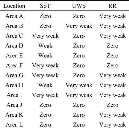
Table 3. Six months variability of indices
Location SST UWS RR
Area I Very weak Very weak Very weak
Area J Zero Zero Zero
Area K Zero Zero Very weak
4.2 The 6 Months Variability
The 3 months moving averages of SST, U-WS and RR identify the signal of the 6 months variability. In the High latitude region, all areas have no 6 months variability of SST and U-WS, except for the area B. The area B shows a very weak 6 months variability of U-WS. All areas in the High latitude region show a very weak 6 months variability of RR.
In the Equatorial region, areas D, E and H show a weak 6 months variability of SST. The other areas in the Equatorial region only show a very weak 6 months variability of SST. The areas H and I show a very weak 6 months variability of U-WS. The other areas in the Equatorial region have no 6 months variability of U-WS. The inner Indonesian Seas, areas D, E and F have no 6 months variability of RR, while the other areas in the Equator show a very weak 6 months variability of RR. It is noted that the ENSO Index area, area J, has no 6 months variability of all indices.
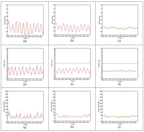
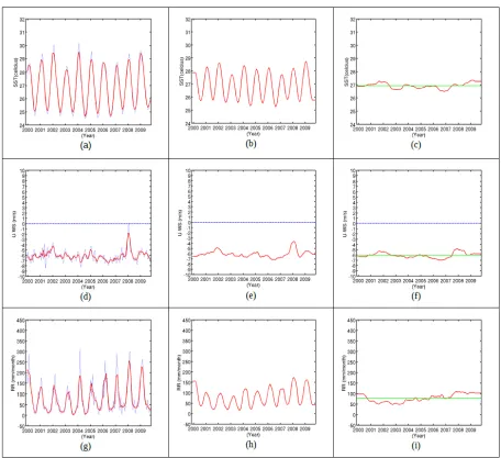
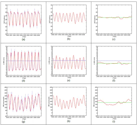
Figure 2. Moving averages of SST (upper panel), U-WS (middle panel) and RR (lower panel) in area A
Figure 3. Moving averages of SST (upper panel), U-WS (middle panel) and RR (lower panel) in area B
Figure 4. Moving averages of SST (upper panel), U-WS (middle panel) and RR (lower panel) in area C
Figure 5. Moving averages of SST (upper panel), U-WS (middle panel) and RR (lower panel) in area D
Figure 6. Moving averages of SST (upper panel), U-WS (middle panel) and RR (lower panel) in area E
Figure 7. Moving averages of SST (upper panel), U-WS (middle panel) and RR (lower panel) in area F
Figure 8. Moving averages of SST (upper panel), U-WS (middle panel) and RR (lower panel) in area G
Figure 9. Moving averages of SST (upper panel), U-WS (middle panel) and RR (lower panel) in area H
Figure 10. Moving averages of SST (upper panel), U-WS (middle panel) and RR (lower panel) in area I
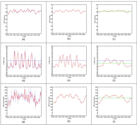
Figure 11. Moving averages of SST (upper panel), U-WS (middle panel) and RR (lower panel) in area J
Figure 12. Moving averages of SST (upper panel), U-WS (middle panel) and RR (lower panel) in area K
Figure 13. Moving averages result of SST (upper panel), U-WS (middle panel) and RR (lower panel) in area L
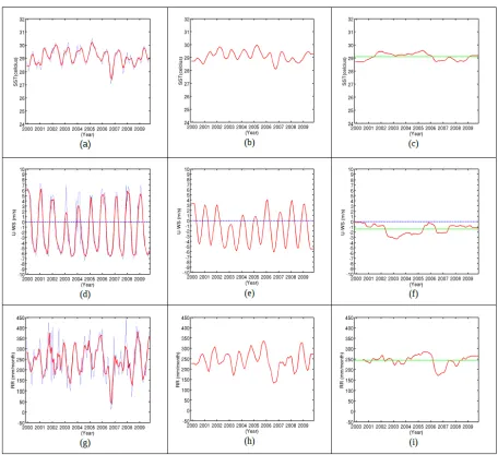
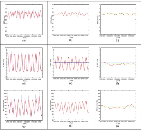
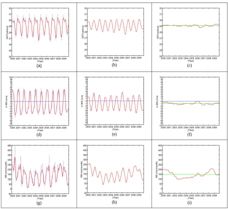
The 3 months moving averages are shown in panel (a), (d) and (g); the 6 months moving averages are shown in panel (b), (e) and (h); the 12 months moving averages are shown in panel (c), (f) and (i). The red line indicates the moving averages result, the blue line indicates the original dataset and the green line indicates the average values. Axes indicate averages of indices and year. The positive values of U-WS indicate eastward direction and vice versa
4.3 The Auto-Correlation and Cross-Correlation Analyses
We further calculate the auto-correlation of SST, U-WS and RR to find out the temporal variability of indices for those areas with a weak seasonal variability: the areas G, H, I and J in the Equatorial Pacific Ocean (see Figures 14 to 16). These areas have no clear temporal variability of SST and RR, except for areas H. The area H shows combined seasonal and 6 months variability of SST. The temporal variability of U-WS in all areas shows the seasonal variability, except for the ENSO Index area, area J.
In the Equatorial region, areas D, E and F (the inner Indonesian Seas) show a strong correlation among indices. The lag time of SST and U-WS for area D is 5 months, while those for areas E and F are 0 month. The lag times of U-WS and RR for areas D, E and F are 0, 2 and 1 months, respectively. The lag time of SST and RR for area D is 0 month, while those for areas E and F are 1 month. The area C only shows a strong correlation between SST and U-WS with 4 months lag times. The ENSO Index area, area J, has no lag time among indices.
(a) (b)
(c) (d)
Figure 14. The auto-correlation of SST within 4 years in area G (panel a), area H (panel b), area I (panel c) and area J (panel d)
(a) (b)
(c) (d)
Figure 15. The auto-correlation of U-WS within 4 years in area G (panel a), area H (panel b), area I (panel c) and area J (panel d)
Axes indicate the correlation values and time lag.
Table 4. Auto-correlation of indices
Location Variability
SST UWS RR
Area G NC 1 Year NC
Area H 6 months 1 Year NC
Area I NC 1 Year NC
(a) (b)
(c) (d)
Figure 16. The auto-correlation of RR within 4 years in area G (panel a), area H (panel b), area I (panel c) and area J (panel d)
Axes indicate the correlation values and time lag.
4.4 The Connection of Indices with ENSO and IOD
The ENSO and IOD indices are defined as SST. We first consider the connection of SST in the Indonesian Seas with the ENSO and IOD signals (see Figures 17 to 20). Based on the comparison, we can discern the effect of the ENSO and IOD signals on the local areas.
In the Pacific Ocean, the areas H and I (the Equatorial region) show both El Nino and La Nina signals of SST. The area G (the Equatorial region) shows La Nina signal but no El Nino signal of SST. The area K (the High latitude region) shows both El Nino and La Nina signals of SST. The area B (the High latitude region) shows El Nino signal but no La Nina signal, while area L (the High latitude region) has no El Nino and no La Nina signals of SST.
In the Indian Ocean, the area A (the High latitude region) has no El Nino and no La Nina signals of SST. The area C (the Equatorial region) shows the El Nino and La Nina signals of SST.
For the response of U-WS and RR, the area A (the High latitude Indian Ocean) only shows the El Nino and La Nina signals of RR. The area C (the Equatorial Indian Ocean) only shows the El Nino and La Nina signals of U-WS. All areas in the High latitude Pacific Ocean show the El Nino and La Nina signals of U-WS and RR, except for the area B. The area B (the High latitude Pacific Ocean) has no El Nino and no La Nina signals of U-WS. All areas in the Equatorial Pacific Ocean and the inner Indonesian Seas show the El Nino and La Nina signals of U-WS and RR.
Table 6. El Nino signal from the 6 months moving averages of the deseasonalized dataset
Location SST UWS RR
02/03 04/05 06/07 02/03 04/05 06/07 02/03 04/05 06/07
Table 7. La Nina signal from the 6 months moving averages of the deseasonalized dataset
Location SST UWS RR
00/01 05/06 07/08 08/09 00/01 05/06 07/08 08/09 00/01 05/06 07/08 08/09
Area A NC NC NC NC NC NC NC NC D NC D D
The D symbol indicates the signal can be detected, while NC indicates the signal is not clear.
Figure 17. The 6 months moving averages of the deseasonalized dataset in area A (left panel), area B (middle panel) and area C (right panel)
Figure 18. The 6 months moving averages of the deseasonalized dataset in area D (left panel), area E (middle panel) and area F (right panel)
Figure 19. The 6 months moving averages of the deseasonalized dataset in area G (left panel), area H (middle panel) and area I (right panel)
Figure 20. The 6 months moving averages of the deseasonalized dataset in area J (left panel), area K (middle panel) and area L (right panel)
The upper panel shows the SST; the middle panel shows the U-WS; and the lower panel shows the RR. The red line indicates the moving averages result and the green line indicates the average values.
4.5 The Local Characteristics
The inner Indonesian Seas, areas D, E and F, show the seasonal variability of all indices. However, the area D has more stable SST than the area E, while both areas have a similar U-WS pattern (see Figures 5 and 6). The difference of SST between areas D and E might be caused by the ocean bathymetry (see Figure 1).
The U-WS in the inner Indonesian Seas switches from west to east and vice versa, while it does not change its direction in the outside areas of the inner Indonesian Seas (see Figures 5 to 7). This is the monsoon wind pattern of the inner Indonesian Seas. Saveral studies have described the monsoon pattern of the inner Indonesian Seas (Wyrtki, 1962; Susanto et al., 2006), but the pattern was unclear (Swardika et al., 2012).
5. Conclusions
Seas. The inner Indonesian Sea only shows the ENSO signal of SST in the year 2007, but it, rather, might be caused by the positive IOD. We show the variabilities and connections of the 12 areas to the ENSO and IOD, but it is difficult to obtain any finding that fits all the areas. One typical locality is the SST difference between the areas D and E.
Figure 21. ENSO years based on ONI dataset. SST is at least 0.5 warmer than 30-year average indicate the El Nino. SST is at least 0.5 cooler than 30-year average indicate the La Nina
Figure 22. Moving averages of DMI dataset. The 3 months moving averages are shown in panel a; the 6 months moving averages are shown in panel b. The red line indicates the moving averages result and the blue line indicates
the original dataset
Acknowledgements
We also thank the Remote Sensing Systems for TRMM-TMI and QuikSCAT data; the Earth Observation Research Center, Japan Aerospace Exploration Agency (JAXA EORC) for precipitation data; and the National Oceanic and Atmospheric Administration (NOAA) - Climate Prediction Center (CPC) for ENSO index data; and the Japan Agency for Marine-Earth Science and Technology (JAMSTEC) for IOD index data.
References
England, M. H., & Fei, H. (2005). On the interannual variability of the Indonesian throughflow and its linkage with ENSO. J. Clim., 18, 1435-1444. http://dx.doi.org/doi:10.1175/JCLI3322.1
Diaz, H. F., Hoerling, M. P., & Eischeid, J. K. (2001). ENSO variability, teleconnections and climate change. Int. J. Climatol., 21, 1845-1862. http://dx.doi.org/doi:10.1002/joc.631
Godfrey, J. S. (1996). The effect of the Indonesian throughflow on ocean circulation and heat exchange with the atmosphere: A review. J. Geophys. Res., 101, 12, 217-12, 237. http://dx.doi.org/doi:10.1029/95JC03860 Gordon, A. L., Susanto, R. D., & Vranes, K. (2003). Cool Indonesian throughflow as a consequence of restricted
surface layer flow. Nature, 425, 824-828. http://dx.doi.org/doi:10.1038/nature02038
Gordon, A. L. (2005). Oceanography of the Indonesian seas and their throughflow. Oceanography, 18(4), 14-27. http://dx.doi.org/doi:10.5670/oceanog.2005.01
Gordon, A., Sprintall, J., Van Aken, H. M., Susanto, D., Wijffels, S., Molcard, R., … Wirasantosa, S., (2010). The Indonesian throughflow during 2004-2006 as observed by the INSTANT program. Dyn. Atmos. Oceans., 50(2), 115-128. http://dx.doi.org/doi:10.1016/j.dynatmoce.2009.12.002
Li, G., Baohua, R., Chengyun, Y., & Jianqiu, Z. (2010). Indices of El Nino and El Nino Modoki: An improved El Nino Modoki index. Adv. Atmos. Sci., 27(5), 1210-1220.
Luo, J. J., Zhang, R., Swadhin, K. B., Yukio, M., Jin, F. F., Roger, L., & Toshio, Y. (2010). Interaction between El Nino and Extreme Indian Ocean Dipole. J. Climate, 23, 726-742. http://dx.doi.org/doi:10.1175/2009JCLI3104.1
Nurweda, P. I. D. N., & Tanaka, T. (2012). Seasonal and inter-annual variability of sea surface temperature and sea surface wind in the eastern part of the Indonesian Sea: ten years analysis of satellite remote sensing data, Proc. SPIE 8525, Remote Sensing of the Marine Environment II, 85250B (December 11, 2012). http://dx.doi.org/doi:10.1117/12.977398
Pradhan, P. K., Preethi, B., Ashok, K., Krishnan, R., & Sahai, A. K. (2011). Modoki, Indian Ocean Dipole, and western North Pacific typhoons: Possible implications for extreme events. J. Geophys. Res., 116, D18108. http://dx.doi.org/doi:10.1029/2011JD015666
Saji, N. H., Goswami, B. N., Vinayachandran, P. N., & Yamagata, T. (1999). A dipole mode in the tropical Indian Ocean. Nature, 401, 360-363. http://dx.doi.org/doi:10.1038/43854
Saji, N. H., & Yamagata, T. (2003). Possible impacts of Indian Ocean Dipole events on global climate. Climate Res., 25, 151-169. http://dx.doi.org/doi:10.3354/cr025151
Smith, W. H. F., & Sandwell, D. T. (1997). Global seafloor topography from satellite altimetry and ship depth soundings. Science, 277, 1957-1962. http://dx.doi.org/doi:10.1126/science.277.5334.1956
Sprintall, J., Susan, W., Gordon, A. L., Amy, F. R., Molcard, R., Susanto, D., … van Aken, H. M. (2004). INSTANT: A New International Array to Measure the Indonesian Throughflow. Eos, 85(39), 369-376. http://dx.doi.org/doi: 10.1029/2004EO390002
Susanto, R. D., Moore II, T. S., & Marra, J. (2006). Ocean color variability in the Indonesia Seas during the SeaWiFS era. Geochemistry, Geophysics, and Geosystems, 7, Q05021. http://dx.doi.org/doi:10.1029/2005GC001009
http://dx.doi.org/doi:10.1007/s00382-009-0658-9
Wyrtki, K. (1962). The upwelling in the region between Java and Australia during the south-east monsoon.
Australian Journal of Marine and Freshwater Research, 13(3), 217-225. http://dx.doi.org/doi:10.1071/MF9620217
Copyrights
Copyright for this article is retained by the author(s), with first publication rights granted to the journal.