Handbook of
Handbook of
Mathematical Formulas
and Integrals
FOURTH EDITION
Alan Jeffrey
Hui-Hui Dai
Professor of Engineering Mathematics Associate Professor of Mathematics University of Newcastle upon Tyne City University of Hong Kong
Newcastle upon Tyne Kowloon, China
United Kingdom
AMSTERDAM•BOSTON•HEIDELBERG•LONDON NEW YORK•OXFORD•PARIS•SAN DIEGO SAN FRANCISCO•SINGAPORE•SYDNEY•TOKYO
Developmental Editor: Mara Vos-Sarmiento Marketing Manager: Leah Ackerson Cover Design: Alisa Andreola Cover Illustration: Dick Hannus
Production Project Manager: Sarah M. Hajduk Compositor: diacriTech
Cover Printer: Phoenix Color Printer: Sheridan Books
Academic Press is an imprint of Elsevier
30 Corporate Drive, Suite 400, Burlington, MA 01803, USA 525 B Street, Suite 1900, San Diego, California 92101-4495, USA 84 Theobald’s Road, London WC1X 8RR, UK
This book is printed on acid-free paper.
Copyright c2008, Elsevier Inc. All rights reserved.
No part of this publication may be reproduced or transmitted in any form or by any means, electronic or mechanical, including photocopy, recording, or any information storage and retrieval system, without permission in writing from the publisher.
Permissions may be sought directly from Elsevier’s Science & Technology Rights Department in Oxford, UK: phone: (+44) 1865 843830, fax: (+44) 1865 853333, E-mail: [email protected]. You may also complete your request online via the Elsevier homepage (http://elsevier.com), by selecting “Support & Contact” then “Copyright and Permission” and then “Obtaining Permissions.”
Library of Congress Cataloging-in-Publication Data Application Submitted
British Library Cataloguing-in-Publication Data
A catalogue record for this book is available from the British Library.
ISBN: 978-0-12-374288-9
For information on all Academic Press publications visit our Web site atwww.books.elsevier.com
Contents
Preface xix
Preface to the Fourth Edition xxi
Notes for Handbook Users xxiii
Index of Special Functions and Notations xliii
0 Quick Reference List of Frequently Used Data 1
0.1. Useful Identities 1
0.1.1. Trigonometric Identities 1
0.1.2. Hyperbolic Identities 2
0.2. Complex Relationships 2
0.3. Constants, Binomial Coefficients and the Pochhammer Symbol 3
0.4. Derivatives of Elementary Functions 3
0.5. Rules of Differentiation and Integration 4
0.6. Standard Integrals 4
0.7. Standard Series 10
0.8. Geometry 12
1 Numerical, Algebraic, and Analytical Results for Series and Calculus 27 1.1. Algebraic Results Involving Real and Complex Numbers 27
1.1.1. Complex Numbers 27
1.1.2. Algebraic Inequalities Involving Real and Complex Numbers 28
1.2. Finite Sums 32
1.2.1. The Binomial Theorem for Positive Integral Exponents 32 1.2.2. Arithmetic, Geometric, and Arithmetic–Geometric Series 36
1.2.3. Sums of Powers of Integers 36
1.2.4. Proof by Mathematical Induction 38
1.3. Bernoulli and Euler Numbers and Polynomials 40
1.3.1. Bernoulli and Euler Numbers 40
1.3.2. Bernoulli and Euler Polynomials 46
1.3.3. The Euler–Maclaurin Summation Formula 48 1.3.4. Accelerating the Convergence of Alternating Series 49
1.4. Determinants 50
1.4.1. Expansion of Second- and Third-Order Determinants 50 1.4.2. Minors, Cofactors, and the Laplace Expansion 51
1.4.3. Basic Properties of Determinants 53
1.4.4. Jacobi’s Theorem 53
1.4.5. Hadamard’s Theorem 54
1.4.6. Hadamard’s Inequality 54
1.4.7. Cramer’s Rule 55
1.4.8. Some Special Determinants 55
1.4.9. Routh–Hurwitz Theorem 57
1.5. Matrices 58
1.5.1. Special Matrices 58
1.5.2. Quadratic Forms 62
1.5.3. Differentiation and Integration of Matrices 64
1.5.4. The Matrix Exponential 65
1.5.5. The Gerschgorin Circle Theorem 67
1.6. Permutations and Combinations 67
1.6.1. Permutations 67
1.6.2. Combinations 68
1.7. Partial Fraction Decomposition 68
1.7.1. Rational Functions 68
1.7.2. Method of Undetermined Coefficients 69
1.8. Convergence of Series 72
1.8.1. Types of Convergence of Numerical Series 72
1.8.2. Convergence Tests 72
1.8.3. Examples of Infinite Numerical Series 74
1.9. Infinite Products 77
1.9.1. Convergence of Infinite Products 77
1.9.2. Examples of Infinite Products 78
1.10. Functional Series 79
1.10.1. Uniform Convergence 79
1.11. Power Series 82
1.11.1. Definition 82
1.12. Taylor Series 86
1.12.1. Definition and Forms of Remainder Term 86 1.12.2. Order Notation (BigOand Littleo) 88
1.13. Fourier Series 89
1.13.1. Definitions 89
1.14. Asymptotic Expansions 93
1.14.1. Introduction 93
1.14.2. Definition and Properties of Asymptotic Series 94
1.15. Basic Results from the Calculus 95
1.15.1. Rules for Differentiation 95
1.15.2. Integration 96
1.15.3. Reduction Formulas 99
1.15.4. Improper Integrals 101
Contents vii
2 Functions and Identities 109
2.1. Complex Numbers and Trigonometric and Hyperbolic Functions 109
2.1.1. Basic Results 109
2.2. Logorithms and Exponentials 121
2.2.1. Basic Functional Relationships 121
2.2.2. The Number e 123
2.3. The Exponential Function 123
2.3.1. Series Representations 123
2.4. Trigonometric Identities 124
2.4.1. Trigonometric Functions 124
2.5. Hyperbolic Identities 132
2.5.1. Hyperbolic Functions 132
2.6. The Logarithm 137
2.6.1. Series Representations 137
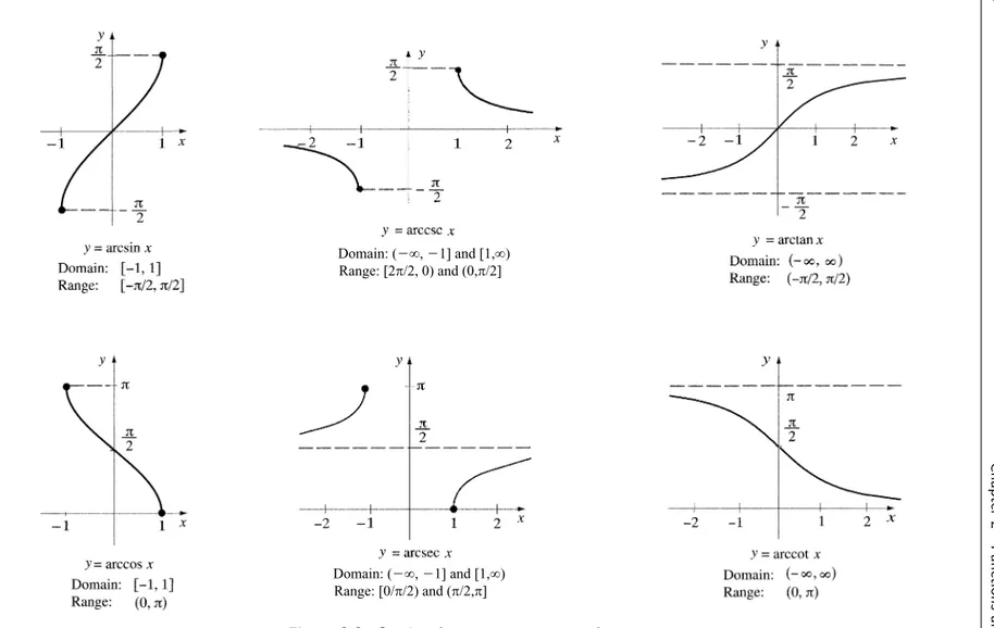
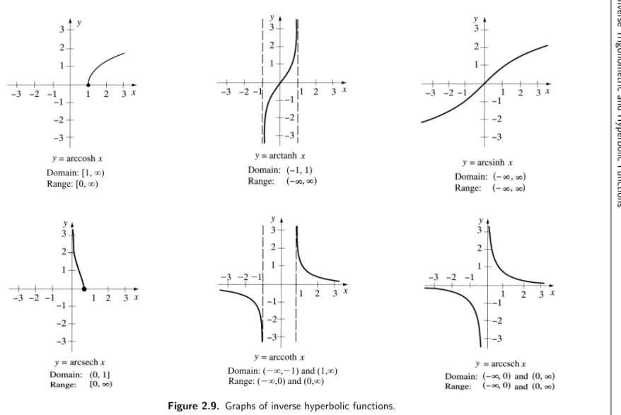
2.7. Inverse Trigonometric and Hyperbolic Functions 139 2.7.1. Domains of Definition and Principal Values 139
2.7.2. Functional Relations 139
2.8. Series Representations of Trigonometric and Hyperbolic Functions 144
2.8.1. Trigonometric Functions 144
2.8.2. Hyperbolic Functions 145
2.8.3. Inverse Trigonometric Functions 146
2.8.4. Inverse Hyperbolic Functions 146
2.9. Useful Limiting Values and Inequalities Involving Elementary Functions 147
2.9.1. Logarithmic Functions 147
2.9.2. Exponential Functions 147
2.9.3. Trigonometric and Hyperbolic Functions 148
3 Derivatives of Elementary Functions 149
3.1. Derivatives of Algebraic, Logarithmic, and Exponential Functions 149
3.2. Derivatives of Trigonometric Functions 150
3.3. Derivatives of Inverse Trigonometric Functions 150
3.4. Derivatives of Hyperbolic Functions 151
3.5. Derivatives of Inverse Hyperbolic Functions 152
4 Indefinite Integrals of Algebraic Functions 153
4.1. Algebraic and Transcendental Functions 153
4.1.1. Definitions 153
4.2. Indefinite Integrals of Rational Functions 154
4.2.1. Integrands Involving xn 154
4.2.2. Integrands Involving a+bx 154
4.2.3. Integrands Involving Linear Factors 157 4.2.4. Integrands Involving a2 ±b2 x2 158
4.2.6. Integrands Involvinga+bx3 164
4.2.7. Integrands Involvinga+bx4 165
4.3. Nonrational Algebraic Functions 166
4.3.1. Integrands Containinga+bxk and√x 166 4.3.2. Integrands Containing (a+bx)1 /2 168 4.3.3. Integrands Containing (a+cx2 )1 /2
170 4.3.4. Integrands Containing
a+bx+cx2 1/2
172
5 Indefinite Integrals of Exponential Functions 175
5.1. Basic Results 175
5.1.1. Indefinite Integrals Involvingeax 175
5.1.2. Integrals Involving the Exponential Functions
Combined with Rational Functions ofx 175 5.1.3. Integrands Involving the Exponential Functions
Combined with Trigonometric Functions 177
6 Indefinite Integrals of Logarithmic Functions 181 6.1. Combinations of Logarithms and Polynomials 181
6.1.1. The Logarithm 181
6.1.2. Integrands Involving Combinations of ln(ax)
and Powers of x 182
6.1.3. Integrands Involving (a+bx)mlnnx 183
6.1.4. Integrands Involving ln(x2 ±a2 ) 185
6.1.5. Integrands Involvingxmlnx+
x2 ±a2 1 /2
186
7 Indefinite Integrals of Hyperbolic Functions 189
7.1. Basic Results 189
7.1.1. Integrands Involving sinh(a+bx) and cosh(a+bx) 189 7.2. Integrands Involving Powers of sinh(bx) or cosh(bx) 190 7.2.1. Integrands Involving Powers of sinh(bx) 190 7.2.2. Integrands Involving Powers of cosh(bx) 190 7.3. Integrands Involving (a+bx)msinh(cx) or (a+bx)mcosh(cx) 191
7.3.1. General Results 191
7.4. Integrands Involvingxmsinhnxor xm coshnx 193
7.4.1. Integrands Involving xmsinhnx 193
7.4.2. Integrands Involving xmcoshnx 193
7.5. Integrands Involvingxmsinhnxor xm coshnx 193
7.5.1. Integrands Involvingxmsinhnx 193
7.5.2. Integrands Involvingxmcoshnx 194
7.6. Integrands Involving (1±coshx)−m 195
7.6.1. Integrands Involving (1±coshx)−1 195
Contents ix
7.7. Integrands Involving sinh(ax) cosh−nxor cosh(ax) sinh−nx 195 7.7.1. Integrands Involving sinh(ax) coshnx 195 7.7.2. Integrands Involving cosh(ax) sinhnx 196 7.8. Integrands Involving sinh(ax+b) and cosh(cx+d) 196
7.8.1. General Case 196
7.8.2. Special Casea=c 197
7.8.3. Integrands Involving sinhpxcoshqx 197 7.9. Integrands Involving tanhkxand cothkx 198
7.9.1. Integrands Involving tanhkx 198
7.9.2. Integrands Involving cothkx 198
7.10. Integrands Involving (a+bx)m sinhkxor (a+bx)m coshkx 199
7.10.1. Integrands Involving (a+bx)msinhkx 199
7.10.2. Integrands Involving (a+bx)mcoshkx 199
8 Indefinite Integrals Involving Inverse Hyperbolic Functions 201
8.1. Basic Results 201
8.1.1. Integrands Involving Products ofxn and
arcsinh(x/a) orarc(x/c) 201
8.2. Integrands Involvingx−n arcsinh(x/a) orx−n arccosh(x/a) 202
8.2.1. Integrands Involvingx−n arcsinh(x/a) 202
8.2.2. Integrands Involvingx−n arccosh(x/a) 203
8.3. Integrands Involving xn arctanh(x/a) orxn arccoth(x/a) 204
8.3.1. Integrands Involvingxn arctanh(x/a) 204
8.3.2. Integrands Involvingxn arccoth(x/a) 204
8.4. Integrands Involving x−n arctanh(x/a) orx−n arccoth(x/a) 205
8.4.1. Integrands Involvingx−n arctanh(x/a) 205
8.4.2. Integrands Involvingx−n arccoth(x/a) 205
9 Indefinite Integrals of Trigonometric Functions 207
9.1. Basic Results 207
9.1.1. Simplification by Means of Substitutions 207 9.2. Integrands Involving Powers ofxand Powers of sinxor cosx 209
9.2.1. Integrands Involvingxnsinmx 209
9.2.2. Integrands Involvingx−nsinmx 210
9.2.3. Integrands Involvingxnsin−mx 211
9.2.4. Integrands Involvingxncosmx 212
9.2.5. Integrands Involvingx−ncosmx 213
9.2.6. Integrands Involvingxncos−mx 213 9.2.7. Integrands Involvingxnsinx/(a+bcosx)m
orxncosx/(a+b sinx)m
214
9.3. Integrands Involving tanxand/or cotx 215
9.4. Integrands Involving sinxand cosx 217 9.4.1. Integrands Involving sinmxcosnx 217
9.4.2. Integrands Involving sin−nx 217
9.4.3. Integrands Involving cos−nx 218
9.4.4. Integrands Involving sinmx/cosnxcosmx/sinnx 218
9.4.5. Integrands Involving sin−mxcos−nx 220
9.5. Integrands Involving Sines and Cosines with Linear
Arguments and Powers ofx 221
9.5.1. Integrands Involving Products of (ax+b)n, sin(cx+d),
and/or cos(px+q) 221
9.5.2. Integrands Involving xnsinmxor xncosmx 222
10 Indefinite Integrals of Inverse Trigonometric Functions 225 10.1. Integrands Involving Powers ofxand Powers of Inverse Trigonometric
Functions 225
10.1.1. Integrands Involvingxn arcsinm(x/a) 225
10.1.2. Integrands Involvingx−n arcsin(x/a) 226
10.1.3. Integrands Involvingxn arccosm(x/a) 226
10.1.4. Integrands Involvingx−n arccos(x/a) 227
10.1.5. Integrands Involvingxn arctan(x/a) 227
10.1.6. Integrands Involvingx−n arctan(x/a) 227
10.1.7. Integrands Involvingxn arccot(x/a) 228
10.1.8. Integrands Involvingx−n arccot(x/a) 228
10.1.9. Integrands Involving Products of Rational
Functions and arccot(x/a) 229
11 The Gamma, Beta, Pi, and Psi Functions, and the Incomplete
Gamma Functions 231
11.1. The Euler Integral Limit and Infinite Product Representations for the Gamma FunctionŴ(x). The Incomplete Gamma Functions
Ŵ(α,x) andγ(α,x) 231
11.1.1. Definitions and Notation 231
11.1.2. Special Properties of Ŵ(x) 232
11.1.3. Asymptotic Representations of Ŵ(x) andn! 233
11.1.4. Special Values of Ŵ(x) 233
11.1.5. The Gamma Function in the Complex Plane 233
11.1.6. The Psi (Digamma) Function 234
11.1.7. The Beta Function 235
11.1.8. Graph ofŴ(x) and Tabular Values ofŴ(x) and lnŴ(x) 235
11.1.9. The Incomplete Gamma Function 236
12 Elliptic Integrals and Functions 241
12.1. Elliptic Integrals 241
Contents xi
12.1.2. Tabulations and Trigonometric Series Representations
of Complete Elliptic Integrals 243
12.1.3. Tabulations and Trigonometric Series forE(ϕ, k) andF(ϕ, k) 245
12.2. Jacobian Elliptic Functions 247
12.2.1. The Functions snu, cnu, and dnu 247
12.2.2. Basic Results 247
12.3. Derivatives and Integrals 249
12.3.1. Derivatives of snu, cnu, and dnu 249 12.3.2. Integrals Involving snu, cnu, and dnu 249
12.4. Inverse Jacobian Elliptic Functions 250
12.4.1. Definitions 250
13 Probability Distributions and Integrals,
and the Error Function 253
13.1. Distributions 253
13.1.1. Definitions 253
13.1.2. Power Series Representations (x≥0) 256
13.1.3. Asymptotic Expansions (x≫0) 256
13.2. The Error Function 257
13.2.1. Definitions 257
13.2.2. Power Series Representation 257
13.2.3. Asymptotic Expansion (x≫0) 257
13.2.4. Connection BetweenP(x) and erfx 258 13.2.5. Integrals Expressible in Terms of erfx 258
13.2.6. Derivatives of erfx 258
13.2.7. Integrals of erfcx 258
13.2.8. Integral and Power Series Representation of in erfcx 259
13.2.9. Value ofin erfcxat zero 259
14 Fresnel Integrals, Sine and Cosine Integrals 261 14.1. Definitions, Series Representations, and Values at Infinity 261
14.1.1. The Fresnel Integrals 261
14.1.2. Series Representations 261
14.1.3. Limiting Values asx→ ∞ 263
14.2. Definitions, Series Representations, and Values at Infinity 263
14.2.1. Sine and Cosine Integrals 263
14.2.2. Series Representations 263
14.2.3. Limiting Values asx→ ∞ 264
15 Definite Integrals 265
15.1. Integrands Involving Powers ofx 265
15.5. Integrands Involving the Logarithmic Function 273 15.6. Integrands Involving the Exponential IntegralEi(x) 274
16 Different Forms of Fourier Series 275
16.1. Fourier Series forf(x) on−π≤x≤π 275
16.1.1. The Fourier Series 275
16.2. Fourier Series forf(x) on−L≤x≤L 276
16.2.1. The Fourier Series 276
16.3. Fourier Series forf(x) ona≤x≤b 276
16.3.1. The Fourier Series 276
16.4. Half-Range Fourier Cosine Series for f(x) on 0≤x≤π 277
16.4.1. The Fourier Series 277
16.5. Half-Range Fourier Cosine Series for f(x) on 0≤x≤L 277
16.5.1. The Fourier Series 277
16.6. Half-Range Fourier Sine Series forf(x) on 0≤x≤π 278
16.6.1. The Fourier Series 278
16.7. Half-Range Fourier Sine Series forf(x) on 0≤x≤L 278
16.7.1. The Fourier Series 278
16.8. Complex (Exponential) Fourier Series forf(x) on−π≤x≤π 279
16.8.1. The Fourier Series 279
16.9. Complex (Exponential) Fourier Series forf(x) on−L≤x≤L 279
16.9.1. The Fourier Series 279
16.10. Representative Examples of Fourier Series 280 16.11. Fourier Series and Discontinuous Functions 285 16.11.1. Periodic Extensions and Convergence of Fourier Series 285 16.11.2. Applications to Closed-Form Summations
of Numerical Series 285
17 Bessel Functions 289
17.1. Bessel’s Differential Equation 289
17.1.1. Different Forms of Bessel’s Equation 289
17.2. Series Expansions forJν(x) andYν(x) 290
17.2.1. Series Expansions for Jn(x) andJν(x) 290
17.2.2. Series Expansions forYn(x) andYν(x) 291
17.2.3. Expansion of sin(x sinθ) and cos(xsinθ) in
Terms of Bessel Functions 292
17.3. Bessel Functions of Fractional Order 292
17.3.1. Bessel FunctionsJ±(n+1 /2 ) (x) 292
17.3.2. Bessel FunctionsY±(n+1 /2 ) (x) 293
17.4. Asymptotic Representations for Bessel Functions 294 17.4.1. Asymptotic Representations for Large Arguments 294 17.4.2. Asymptotic Representation for Large Orders 294
17.5. Zeros of Bessel Functions 294
Contents xiii
17.6. Bessel’s Modified Equation 294
17.6.1. Different Forms of Bessel’s Modified Equation 294
17.7. Series Expansions forIν(x) andKν(x) 297
17.7.1. Series Expansions forIn(x) andIν(x) 297
17.7.2. Series Expansions forK0 (x) andKn(x) 298
17.8. Modified Bessel Functions of Fractional Order 298 17.8.1. Modified Bessel FunctionsI±(n+1 /2 ) (x) 298
17.8.2. Modified Bessel FunctionsK±(n+1 /2 ) (x) 299
17.9. Asymptotic Representations of Modified Bessel Functions 299 17.9.1. Asymptotic Representations for Large Arguments 299 17.10. Relationships Between Bessel Functions 299 17.10.1. Relationships InvolvingJν(x) andYν(x) 299 17.10.2. Relationships InvolvingIν(x) andKν(x) 301 17.11. Integral Representations ofJn(x),In(x), andKn(x) 302
17.11.1. Integral Representations ofJn(x) 302
17.12. Indefinite Integrals of Bessel Functions 302 17.12.1. Integrals ofJn(x),In(x), andKn(x) 302
17.13. Definite Integrals Involving Bessel Functions 303 17.13.1. Definite Integrals InvolvingJn(x) and Elementary Functions 303
17.14. Spherical Bessel Functions 304
17.14.1. The Differential Equation 304
17.14.2. The Spherical Bessel Functionjn(x) andyn(x) 305
17.14.3. Recurrence Relations 306
17.14.4. Series Representations 306
17.14.5. Limiting Values asx→0 306
17.14.6. Asymptotic Expansions ofjn(x) andyn(x)
When the OrdernIs Large 307
17.15. Fourier-Bessel Expansions 307
18 Orthogonal Polynomials 309
18.1. Introduction 309
18.1.1. Definition of a System of Orthogonal Polynomials 309
18.2. Legendre PolynomialsPn(x) 310
18.2.1. Differential Equation Satisfied byPn(x) 310
18.2.2. Rodrigues’ Formula for Pn(x) 310
18.2.3. Orthogonality Relation for Pn(x) 310
18.2.4. Explicit Expressions forPn(x) 310
18.2.5. Recurrence Relations Satisfied byPn(x) 312
18.2.6. Generating Function forPn(x) 313
18.2.7. Legendre Functions of the Second Kind Qn(x) 313
18.2.8. Definite Integrals InvolvingPn(x) 315
18.2.10. Associated Legendre Functions 316
18.2.11. Spherical Harmonics 318
18.3. Chebyshev PolynomialsTn(x) andUn(x) 320
18.3.1. Differential Equation Satisfied byTn(x) andUn(x) 320
18.3.2. Rodrigues’ Formulas forTn(x) andUn(x) 320
18.3.3. Orthogonality Relations forTn(x) andUn(x) 320
18.3.4. Explicit Expressions forTn(x) andUn(x) 321
18.3.5. Recurrence Relations Satisfied byTn(x) andUn(x) 325
18.3.6. Generating Functions forTn(x) andUn(x) 325
18.4. Laguerre PolynomialsLn(x) 325
18.4.1. Differential Equation Satisfied byLn(x) 325
18.4.2. Rodrigues’ Formula forLn(x) 325
18.4.3. Orthogonality Relation forLn(x) 326
18.4.4. Explicit Expressions forLn(x) andxn in
Terms ofLn(x) 326
18.4.5. Recurrence Relations Satisfied byLn(x) 327
18.4.6. Generating Function forLn(x) 327
18.4.7. Integrals InvolvingLn(x) 327
18.4.8. Generalized (Associated) Laguerre Polynomials
L(nα)(x) 327
18.5. Hermite PolynomialsHn(x) 329
18.5.1. Differential Equation Satisfied byHn(x) 329
18.5.2. Rodrigues’ Formula forHn(x) 329
18.5.3. Orthogonality Relation forHn(x) 330
18.5.4. Explicit Expressions forHn(x) 330
18.5.5. Recurrence Relations Satisfied byHn(x) 330
18.5.6. Generating Function forHn(x) 331
18.5.7. Series Expansions ofHn(x) 331
18.5.8. Powers ofxin Terms ofHn(x) 331
18.5.9. Definite Integrals 331
18.5.10. Asymptotic Expansion for Largen 332
18.6. Jacobi PolynomialsPn(α,β)(x) 332
18.6.1. Differential Equation Satisfied byPn(α,β) (x) 333
18.6.2. Rodrigues’ Formula forPn(α,β)(x) 333
18.6.3. Orthogonality Relation forPn(α,β)(x) 333
18.6.4. A Useful Integral InvolvingPn(α,β) (x) 333
18.6.5. Explicit Expressions forPn(α,β)(x) 333
18.6.6. Differentiation Formulas forPn(α,β) (x) 334
18.6.7. Recurrence Relation Satisfied byPn(α,β) (x) 334
18.6.8. The Generating Function forPn(α,β)(x) 334
18.6.9. Asymptotic Formula forPn(α,β)(x) for Large n 335
Contents xv
19 Laplace Transformation 337
19.1. Introduction 337
19.1.1. Definition of the Laplace Transform 337 19.1.2. Basic Properties of the Laplace Transform 338
19.1.3. The Dirac Delta Functionδ(x) 340
19.1.4. Laplace Transform Pairs 340
19.1.5. Solving Initial Value Problems by the Laplace
Transform 340
20 Fourier Transforms 353
20.1. Introduction 353
20.1.1. Fourier Exponential Transform 353
20.1.2. Basic Properties of the Fourier Transforms 354
20.1.3. Fourier Transform Pairs 355
20.1.4. Fourier Cosine and Sine Transforms 357 20.1.5. Basic Properties of the Fourier Cosine and Sine
Transforms 358
20.1.6. Fourier Cosine and Sine Transform Pairs 359
21 Numerical Integration 363
21.1. Classical Methods 363
21.1.1. Open- and Closed-Type Formulas 363
21.1.2. Composite Midpoint Rule (open type) 364 21.1.3. Composite Trapezoidal Rule (closed type) 364 21.1.4. Composite Simpson’s Rule (closed type) 364
21.1.5. Newton–Cotes formulas 365
21.1.6. Gaussian Quadrature (open-type) 366
21.1.7. Romberg Integration (closed-type) 367
22 Solutions of Standard Ordinary Differential
Equations 371
22.1. Introduction 371
22.1.1. Basic Definitions 371
22.1.2. Linear Dependence and Independence 371
22.2. Separation of Variables 373
22.3. Linear First-Order Equations 373
22.4. Bernoulli’s Equation 374
22.5. Exact Equations 375
22.6. Homogeneous Equations 376
22.7. Linear Differential Equations 376
22.8. Constant Coefficient Linear Differential
Equations—Homogeneous Case 377
22.10. Linear Differential Equations—Inhomogeneous Case
and the Green’s Function 382
22.11. Linear Inhomogeneous Second-Order Equation 389 22.12. Determination of Particular Integrals by the Method
of Undetermined Coefficients 390
22.13. The Cauchy–Euler Equation 393
22.14. Legendre’s Equation 394
22.15. Bessel’s Equations 394
22.16. Power Series and Frobenius Methods 396
22.17. The Hypergeometric Equation 403
22.18. Numerical Methods 404
23 Vector Analysis 415
23.1. Scalars and Vectors 415
23.1.1. Basic Definitions 415
23.1.2. Vector Addition and Subtraction 417
23.1.3. Scaling Vectors 418
23.1.4. Vectors in Component Form 419
23.2. Scalar Products 420
23.3. Vector Products 421
23.4. Triple Products 422
23.5. Products of Four Vectors 423
23.6. Derivatives of Vector Functions of a Scalart 423 23.7. Derivatives of Vector Functions of Several Scalar Variables 425 23.8. Integrals of Vector Functions of a Scalar Variablet 426
23.9. Line Integrals 427
23.10. Vector Integral Theorems 428
23.11. A Vector Rate of Change Theorem 431
23.12. Useful Vector Identities and Results 431
24 Systems of Orthogonal Coordinates 433
24.1. Curvilinear Coordinates 433
24.1.1. Basic Definitions 433
24.2. Vector Operators in Orthogonal Coordinates 435
24.3. Systems of Orthogonal Coordinates 436
25 Partial Differential Equations and Special Functions 447
25.1. Fundamental Ideas 447
25.1.1. Classification of Equations 447
25.2. Method of Separation of Variables 451
Contents xvii
25.5. Conservation Equations (Laws) 457
25.6. The Method of Characteristics 458
25.7. Discontinuous Solutions (Shocks) 462
25.8. Similarity Solutions 465
25.9. Burgers’s Equation, the KdV Equation, and the KdVB Equation 467
25.10. The Poisson Integral Formulas 470
25.11. The Riemann Method 471
26 Qualitative Properties of the Heat and Laplace Equation 473 26.1. The Weak Maximum/Minimum Principle for the Heat Equation 473 26.2. The Maximum/Minimum Principle for the Laplace Equation 473 26.3. Gauss Mean Value Theorem for Harmonic Functions in the Plane 473 26.4. Gauss Mean Value Theorem for Harmonic Functions in Space 474
27 Solutions of Elliptic, Parabolic, and Hyperbolic Equations 475 27.1. Elliptic Equations (The Laplace Equation) 475 27.2. Parabolic Equations (The Heat or Diffusion Equation) 482
27.3. Hyperbolic Equations (Wave Equation) 488
28 The z-Transform 493
28.1. Thez-Transform and Transform Pairs 493
29 Numerical Approximation 499
29.1. Introduction 499
29.1.1. Linear Interpolation 499
29.1.2. Lagrange Polynomial Interpolation 500
29.1.3. Spline Interpolation 500
29.2. Economization of Series 501
29.3. Pad´e Approximation 503
29.4. Finite Difference Approximations to Ordinary and Partial Derivatives 505
30 Conformal Mapping and Boundary Value Problems 509 30.1. Analytic Functions and the Cauchy-Riemann Equations 509 30.2. Harmonic Conjugates and the Laplace Equation 510 30.3. Conformal Transformations and Orthogonal Trajectories 510
30.4. Boundary Value Problems 511
30.5. Some Useful Conformal Mappings 512
Short Classified Reference List 525
Preface
This book contains a collection of general mathematical results, formulas, and integrals that occur throughout applications of mathematics. Many of the entries are based on the updated fifth edition of Gradshteyn and Ryzhik’s ”Tables of Integrals, Series, and Products,” though during the preparation of the book, results were also taken from various other reference works. The material has been arranged in a straightforward manner, and for the convenience of the user a quick reference list of the simplest and most frequently used results is to be found in Chapter 0 at the front of the book. Tab marks have been added to pages to identify the twelve main subject areas into which the entries have been divided and also to indicate the main interconnections that exist between them. Keys to the tab marks are to be found inside the front and back covers.
The Table of Contents at the front of the book is sufficiently detailed to enable rapid location of the section in which a specific entry is to be found, and this information is supplemented by a detailed index at the end of the book. In the chapters listing integrals, instead of displaying them in their canonical form, as is customary in reference works, in order to make the tables more convenient to use, the integrands are presented in the more general form in which they are likely to arise. It is hoped that this will save the user the necessity of reducing a result to a canonical form before consulting the tables. Wherever it might be helpful, material has been added explaining the idea underlying a section or describing simple techniques that are often useful in the application of its results.
Standard notations have been used for functions, and a list of these together with their names and a reference to the section in which they occur or are defined is to be found at the front of the book. As is customary with tables of indefinite integrals, the additive arbitrary constant of integration has always been omitted. The result of an integration may take more than one form, often depending on the method used for its evaluation, so only the most common forms are listed.
A user requiring more extensive tables, or results involving the less familiar special functions, is referred to the short classified reference list at the end of the book. The list contains works the author found to be most useful and which a user is likely to find readily accessible in a library, but it is in no sense a comprehensive bibliography. Further specialist references are to be found in the bibliographies contained in these reference works.
Every effort has been made to ensure the accuracy of these tables and, whenever possible, results have been checked by means of computer symbolic algebra and integration programs, but the final responsibility for errors must rest with the author.
Preface to the Fourth Edition
The preparation of the fourth edition of this handbook provided the opportunity to enlarge the sections on special functions and orthogonal polynomials, as suggested by many users of the third edition. A number of substantial additions have also been made elsewhere, like the enhancement of the description of spherical harmonics, but a major change is the inclusion of a completely new chapter on conformal mapping. Some minor changes that have been made are correcting of a few typographical errors and rearranging the last four chapters of the third edition into a more convenient form. A significant development that occurred during the later stages of preparation of this fourth edition was that my friend and colleague Dr. Hui-Hui Dai joined me as a co-editor.
Chapter 30 on conformal mapping has been included because of its relevance to the solu-tion of the Laplace equasolu-tion in the plane. To demonstrate the connecsolu-tion with the Laplace equation, the chapter is preceded by a brief introduction that demonstrates the relevance of conformal mapping to the solution of boundary value problems for real harmonic functions in the plane. Chapter 30 contains an extensive atlas of useful mappings that display, in the usual diagrammatic way, how given analytic functionsw=f(z) map regions of interest in the complexz-plane onto corresponding regions in the complexw-plane, and conversely. By form-ing composite mappform-ings, the basic atlas of mappform-ings can be extended to more complicated regions than those that have been listed. The development of a typical composite mapping is illustrated by using mappings from the atlas to construct a mapping with the property that a region of complicated shape in thez-plane is mapped onto the much simpler region compris-ing the upper half of thew-plane. By combining this result with the Poisson integral formula, described in another section of the handbook, a boundary value problem for the original, more complicated region can be solved in terms of a corresponding boundary value problem in the simpler region comprising the upper half of thew-plane.
The chapter on ordinary differential equations has been enhanced by the inclusion of mate-rial describing the construction and use of the Green’s function when solving initial and boundary value problems for linear second order ordinary differential equations. More has been added about the properties of the Laplace transform and the Laplace and Fourier con-volution theorems, and the list of Laplace transform pairs has been enlarged. Furthermore, because of their use with special techniques in numerical analysis when solving differential equations, a new section has been included describing the Jacobi orthogonal polynomials. The section on the Poisson integral formulas has also been enlarged, and its use is illustrated by an example. A brief description of the Riemann method for the solution of hyperbolic equations has been included because of the important theoretical role it plays when examining general properties of wave-type equations, such as their domains of dependence.
For the convenience of users, a new feature of the handbook is a CD-ROM that contains the classified lists of integrals found in the book. These lists can be searched manually, and when results of interest have been located, they can be either printed out or used in papers or
worksheets as required. This electronic material is introduced by a set of notes (also included in the following pages) intended to help users of the handbook by drawing attention to different notations and conventions that are in current use. If these are not properly understood, they can cause confusion when results from some other sources are combined with results from this handbook. Typically, confusion can occur when dealing with Laplace’s equation and other second order linear partial differential equations using spherical polar coordinates because of the occurrence of differing notations for the angles involved and also when working with Fourier transforms for which definitions and normalizations differ. Some explanatory notes and examples have also been provided to interpret the meaning and use of the inversion integrals for Laplace and Fourier transforms.
Alan Jeffrey [email protected]
Notes for Handbook Users
The material contained in the fourth edition of theHandbook of Mathematical Formulas and Integrals was selected because it covers the main areas of mathematics that find frequent use in applied mathematics, physics, engineering, and other subjects that use mathematics. The material contained in the handbook includes, among other topics, algebra, calculus, indefinite and definite integrals, differential equations, integral transforms, and special functions.
For the convenience of the user, the most frequently consulted chapters of the book are to be found on the accompanying CD that allows individual results of interest to be printed out, included in a work sheet, or in a manuscript.
A major part of the handbook concerns integrals, so it is appropriate that mention of these should be made first. As is customary, when listing indefinite integrals, the arbitrary additive constant of integration has always been omitted. The results concerning integrals that are available in the mathematical literature are so numerous that a strict selection process had to be adopted when compiling this work. The criterion used amounted to choosing those results that experience suggested were likely to be the most useful in everyday applications of mathematics. To economize on space, when a simple transformation can convert an integral containing several parameters into one or more integrals with fewer parameters, only these simpler integrals have been listed.
For example, instead of listing indefinite integrals like
eaxsin(bx+c)dx and eax
cos(bx+c)dx, each containing the three parameters a, b, and c, the simpler indefinite inte-grals
eaxsinbxdx and
eaxcosbxdx contained in entries 5.1.3.1(1) and 5.1.3.1(4) have
been listed. The results containing the parameter c then follow after using additive prop-erty of integrals with these tabulated entries, together with the trigonometric identities sin(bx+c) = sinbxcosc+ cosbxsincand cos(bx+c) = cosbxcosc−sinbxsinc.
The order in which integrals are listed can be seen from the various section headings. If a required integral is not found in the appropriate section, it is possible that it can be transformed into an entry contained in the book by using one of the following elementary methods:
1. Representing the integrand in terms of partial fractions.
2. Completing the square in denominators containing quadratic factors. 3. Integration using a substitution.
4. Integration by parts.
5. Integration using a recurrence relation (recursion formula),
or by a combination of these. It must, however, always be remembered that not all integrals can be evaluated in terms of elementary functions. Consequently, many simple looking integrals cannot be evaluated analytically, as is the case with
sinx a+bexdx.
A Comment on the Use of Substitutions
When using substitutions, it is important to ensure the substitution is both continuous and one-to-one, and to remember to incorporate the substitution into thedxterm in the integrand. When a definite integral is involved the substitution must also be incorporated into the limits of the integral.
When an integrand involves an expression of the form √a2 −x2 , it is usual to use the
substitution x=|asinθ| which is equivalent to θ= arcsin(x/|a|), though the substitution x=|a|cosθwould serve equally well. The occurrence of an expression of the form√a2 +x2 in
an integrand can be treated by making the substitution x=|a|tanθ, whenθ= arctan(x/|a|) (see also Section 9.1.1). If an expression of the form √x2 −a2 occurs in an integrand, the
substitutionx=|a|secθcan be used. Notice that whenever the square root occurs thepositive square root is always implied, to ensure that the function is single valued.
If a substitution involving either sinθ or cosθ is used, it is necessary to restrict θ to a suitable interval to ensure the substitution remains one-to-one. For example, by restricting θ to the interval−21 π≤θ≤
1
2 π, the function sinθbecomes one-to-one, whereas by restricting θ
to the interval 0≤θ≤π, the function cosθbecomes one-to-one. Similarly, when the inverse trigonometric function y= arcsinxis involved, equivalent to x= siny, the function becomes one-to-one in its principal branch −1
2 π≤y≤
1
2 π, so arcsin(sinx) =x for −
1
2 π≤x≤
1
2 π
and sin(arcsinx) =x for −1≤x≤1. Correspondingly, the inverse trigonometric function y= arccosx, equivalently x= cosy, becomes one-to-one in its principal branch 0≤y≤π, so arccos(cosx) =xfor 0≤x≤πand sin(arccosx) =xfor−1≤x≤1.
It is important to recognize that a given integral may have more than one representation, because the form of the result is often determined by the method used to evaluate the integral. Some representations are more convenient to use than others so, where appropriate, integrals of this type are listed using their simplest representation. A typical example of this type is
dx
√
a2 +x2 =
arcsinh(x/a)
ln
x+√a2 +x2
where the result involving the logarithmic function is usually the more convenient of the two forms. In this handbook, both the inverse trigonometric and inverse hyperbolic functions all carry the prefix “arc.” So, for example, the inverse sine function is written arcsin x and the inverse hyperbolic sine function is written arcsinhx, with corresponding notational conventions for the other inverse trigonometric and hyperbolic functions. However, many other works denote the inverse of these functions by adding the superscript−1 to the name of the function,
Notes for Handbook Users xxv
function, the prefix “arg” is used, so that arcsinhxbecomes argsinhx, with the corresponding use of the prefix “arg” to denote the other inverse hyperbolic functions. This notation is preferred by some authors because they consider that the prefix “arc” implies an angle is involved, whereas this is not the case with hyperbolic functions. So, instead, they use the prefix “arg” when working with inverse hyperbolic functions.
Example: FindI= x5 √
a2 −x2dx.
Of the two obvious substitutionsx=|a|sinθandx=|a|cosθthat can be used, we will make use of the first one, while remembering to restrict θto the interval −1
2 π≤θ≤
1
2 π to ensure
the transformation is one-to-one. We havedx=|a|cosθdθ, while√a2 −x2 =a2 −a2 sin2 θ=
|a|1−sin2 θ=|acosθ|. However cosθis positive in the interval −1
2 π≤θ≤
1
2 π, so we may
set√a2 −x2 =|a|cosθ. Substituting these results into the integrand of I gives
I=
|a|5 sin5 θ|a|cosθdθ |a|cosθ =a
4
|a|
sin5 θdθ,
and this trigonometric integral can be found using entry9.2.2.2, 5. This result can be expressed in terms ofxby using the fact thatθ= arcsin (x/|a|), so that after some manipulation we find that
I=−1 5x
4
a2 −x2 −4a
2
15
a2 −x2
2a2 +x2 .
A Comment on Integration by Parts
Integration by parts can often be used to express an integral in a simpler form, but it also has another important property because it also leads to the derivation of areduction formula, also called arecursion relation. A reduction formula expresses an integral involving one or more parameters in terms of a simpler integral of the same form, but with the parameters having smaller values. Let us consider two examples in some detail, the second of which given a brief mention in Section1.15.3.
Example:
(a) Find a reduction formula for
Im=
cosmθdθ,
and hence find an expression forI5 .
(b) Modify the result to find a recurrence relation for
Jm=
π/2
0
cosmθdθ,
To derive the result for (a), write
Im=
cosm−1 θd(sinθ) dθ dθ
= cosm−1 θsinθ−
sinθ(m−1) cosm−2 θ(−sinθ)dθ
= cosm−1 θsinθ+ (m−1)
cosm−2 θ(1−cos2 θ)dθ
= cosm−1 θsinθ+ (m−1)
cosm−2 θdθ−(m−1)
cosmθdθ.
Combining terms and using the form ofIm, this gives the reduction formula
Im=
cosm−1 θsinθ
m +
m−1 m
Im−2 .
we have I1 =cosθdθ= sinθ. So using the expression for I1 , setting m= 5 and using the
recurrence relation to step up in intervals of 2, we find that
I3 =
1 3cos
2 θsinθ+2
3I1 = 1 3cos
2 θ+2
3sinθ,
and hence that
I5 =
1 5cos
4 θsinθ+4
5I3
= 1 5cos
4 θsinθ− 4
15sin
3
θ+4 5sinθ.
The derivation of a result for (b) uses the same reasoning as in (a), apart from the fact that the limits must be applied to both the integral, and also to theuνterm in
udν=uν−νdu, so the result becomes b
audν= (uν) b a−
b
a νdu. When this is done it leads to the result
Jm=
cosm−1 θsinθ
m
π/2
θ=0
+ m−1 m
Jm−2 =
m−1 m
Jm−2 .
Whenmis even, this recurrence relation linksJmtoJ0 =0π/2 1dθ=12 π, and whenmis odd,
it linksJmtoJ1 =0π/2 cosθdθ= 1. Using these results sequentially in the recurrence relation,
we find that
J2 n=
1·3·5. . .(2n−1) 2·4·6. . .2n
1
2π, (m= 2nis even)
and
J2 n+1 = 2·4·6. . .2n
Notes for Handbook Users xxvii
Example: The following is an example of a recurrence formula that contains two param-eters. If Im,n=sinmθcosnθdθ, an argument along the lines of the one used in the previous
example, but writing
Im,n=
sinm−1 θcosnθd(−cosθ),
leads to the result
(m+n)Im,n=−sinm−1 θcosn+1 θ+ (m−1)Im−2 ,n,
in whichnremains unchanged, butmdecreases by 2.
Had integration by parts been used differently withIm,nwritten as
Im,n=
sinmθcosn−1 θd(sinθ)
a different reduction formula would have been obtained in whichmremains unchanged butn decreases by 2.
Some Comments on Definite Integrals
Definite integrals evaluated over the semi-infinite interval [0,∞) or over the infinite interval (−∞,∞) are improper integrals and when they are convergent they can often be evaluated by means of contour integration. However, when considering these improper integrals, it is desirable to know in advance if they are convergent, or if they only have a finite value in the sense of a Cauchy principal value. (see Section1.15.4). A geometrical interpretation of a Cauchy principal value for an integral of a functionf(x) over the interval (−∞,∞) follows by regarding an area between the curvey=f(x) and thex-axis as positive if it lies above the x-axis and negative if it lies below it. Then, when finding a Cauchy principal value, the areas to the left and right of they-axis are paired off symmetrically as the limits of integration approach ±∞. If the result is a finite number, this is the Cauchy principal value to be attributed to the definite integral ∞
−∞f(x)dx, otherwise the integral is divergent. When an improper integral is convergent, its value and its Cauchy principal value coincide.
There are various tests for the convergence of improper integrals, but the ones due to Abel and Dirichlet given in Section 1.15.4 are the main ones. Convergent integrals exist that do not satisfy all of the conditions of the theorems, showing that although these tests represent sufficient conditions for convergence, they arenot necessary ones.
Example: Let us establish the convergence of the improper integral∞
a s i n mx
xp dx, given that a, p >0.
To use the Dirichlet test we set f(x) = sinx and g(x) = 1/xp. Then lim
x→∞g(x) = 0 and ∞
a |g′(x)|dx= 1/a
p is finite, so this integral involving g(x) converges. We also have
F(b) =b
a≤x≤b <∞. Thus the conditions of the Dirichlet test are satisfied showing that∞
a s i n x
xp dx is convergent fora, p >0.
It is necessary to exercise caution when using the fundamental theorem of calculus to evaluate an improper integral in case the integrand has a singularity (becomes infinite) inside the interval of integration. If this occurs the use of the fundamental theorem of calculus is invalid.
Example: The improper integrala −a
dx
x2 witha >0 has a singularity at the origin and is, in fact, divergent. This follows because ifε,δ>0, we have lim
ε→0
−ε −a
dx x2 + lim
δ→0
b δ
dx
x2 =∞. However, an incorrect application of the fundamental theorem of calculus gives a
−a dx x2 =
−1
x
a
x=−a=
−2
a. Although this result is finite, it is obviously incorrect because the integrand is positive
over the interval of integration, so the definite integral must also be positive, but this is not the case here becausea >0 so−2/a <0.
Two simple results that often save time concern the integration of even and odd functions f(x) over an interval−a≤x≤athat is symmetrical about the origin.
We have the obvious result that whenf(x) isodd, that is whenf(−x) =−f(x), then
a
−a
f(x)dx= 0,
and whenf(x) is even, that is when f(−x) =f(x),then
a
−a
f(x)dx= 2 a
0
f(x)dx.
These simple results have many uses as, for example, when working with Fourier series and elsewhere.
Some Comments on Notations, the Choice of Symbols, and Normalization
Unfortunately there is no universal agreement on the choice of symbols used to identify a point P in cylindrical and spherical polar coordinates. Nor is there universal agreement on the choice of symbols used to represent some special functions, or on the normalization of Fourier transforms. Accordingly, before using results derived from other sources with those given in this handbook, it is necessary to check the notations, symbols, and normalization used elsewhere prior to combining the results.Symbols Used with Curvilinear Coordinates
Notes for Handbook Users xxix
The plane polar coordinates(r,θ) that identify a pointP in the (x,y)-plane are shown in Figure 1(a). The angleθis theazimuthal angle measured counterclockwise from thex-axis in the (x,y)-plane to the radius vectorrdrawn from the origin to the pointP. The connection between the Cartesian and the plane polar coordinates ofP is given byx=rcosθ, y=rsinθ, with 0≤θ<2π.
0
y
r
x
P(r,)
Figure 1(a)
We mention here that a different convention denotes the azimuthal angle in plane polar coordinates byθ, instead of byφ.
The cylindrical polar coordinates(r,θ, z) that identify a pointP in space are shown in Figure 1(b). The angleθis again theazimuthal anglemeasured as in plane polar coordinates, r is the radial distance measured from the origin in the (x,y)-plane to the projection of P onto the (x,y)-plane, and z is the perpendicular distance of P above the (x,y)-plane. The connection between cartesian and cylindrical polar coordinates used in this handbook is given byx=rcosθ, y=rsinθandz=z, with 0≤θ<2π.
0
z
z
y
x
P(r,, z)
r
Here also, in a different convention involving cylindrical polar coordinates, the azimuthal angle is denoted by φinstead of by θ.
The spherical polar coordinates(r,θ,φ) that identify a pointP in space are shown in Fig-ure 1(c). Here, differently from plane cylindrical coordinates, theazimuthal anglemeasured as in plane cylindrical coordinates is denoted byφ, the radiusris measured from the origin to point P, and the polar anglemeasured from the z-axis to the radius vectorOP is denoted by θ, with 0≤φ<2π, and 0≤θ≤π. The cartesian and spherical polar coordinates used in this handbook are connected byx=rsinθcosφ, y=rsinθsinφ, z=rcosθ.
0 z
y
x
P(r, , )
Figure 1(c)
In a different convention the roles ofθandφare interchanged, so the azimuthal angle is denoted byθ, and the polar angle is denoted byφ.
Bessel Functions
Notes for Handbook Users xxxi
method, the nature of the solution takes one form when ν is an integer and a different one when νis not an integer. The form of definition of Yν(x) used here overcomes this difficulty because it is valid for allν.
The recurrence relations for all Bessel functions can be written as
Zν−1 (x) +Zν+1 (x) =
2ν xZν(x), Zν−1 (x)−Zν+1 (x) = 2Zν′(x),
Z′
ν(x) =Zν−1 (x)− ν xZν(x)′ Z′
ν(x) =−Zν+1 (x) + ν xZν(x),
(1)
where Zν(x) can be either Jν(x) orYν(x). Thus any recurrence relation derived from these results will apply to all Bessel functions. Similar general results exist for the modified Bessel functionsIν(x) andKν(x).
Normalization of Fourier Transforms
The convention adopted in this handbook is to define the Fourier transformof a function f(x) as the function F(ω) where
F(ω) =√1 2π
∞
−∞
f(x)eiωxdx, (2)
when theinverse Fourier transformbecomes f(x) = √1
2π
∞
−∞
F(ω)e−iωxdω, (3)
where the normalization factor multiplying each integral in this Fourier transform pair is 1/√2π.However other conventions for the normalization are in common use, and they follow from the requirement that the product of the two normalization factors in the Fourier and inverse Fourier transforms must equal 1/(2π).
Thus another convention that is used defines the Fourier transform off(x) as
F(ω) = ∞
−∞
f(x)eiωxdx (4)
and the inverse Fourier transform as
f(x) = 1 2π
∞
−∞
F(ω)e−iωxdω. (5)
To complicate matters still further, in some conventions the factoreiωxin the integral defining
F(ω) is replaced by e−iωx and to compensate the factore−iωx in the integral definingf(x) is
If a Fourier transform is defined in terms of an angular frequency, the ambiguity concerning the choice of normalization factors disappears because the Fourier transform of f(x) becomes
F(ω) = ∞
−∞
f(x)e2 πixsdx (6)
and the inverse Fourier transform becomes
f(x) = ∞
−∞
F(ω)e−2 πixωdω. (7)
Nevertheless, the difference between definitions still continues because sometimes the expo-nential factor in F(s) is replaced by e−2 πixs, in which case the corresponding factor in the
inverse Fourier transform becomes e2 πixs. These remarks should suffice to convince a reader
of the necessity to check the convention used before combining a Fourier transform pair from another source with results from this handbook.
Some Remarks Concerning Elementary Ways of Finding Inverse
Laplace Transforms
The Laplace transform F(s) of a suitably integrable function f(x) is defined by the improper integral
F(s) = ∞
0
f(x)e−xsdx. (8)
Let a Laplace transformF(s) be the quotientF(s) =P(s)/Q(s) of two polynomialsP(s) and Q(s). Finding the inverse transform L−1 {F(s)}=f(x) can be accomplished by simplifying
F(s) using partial fractions, and then using the Laplace transform pairs in Table 19.1 together with the operational properties of the transform given in 19.1.2.1. Notice that the degree of P(s) must be less than the degree ofQ(s) because from the limiting condition in19.11.2.1(10), ifF(s) is to be a Laplace transform of some function f(x), it is necessary that lim
s→∞F(s) = 0. The same approach is valid if exponential terms of the typee−as occur in the numeratorP(s)
because depending on the form of the partial fraction representation ofF(s), such terms will simply introduce either a Heaviside step functionH(x−a), or a Dirac delta functionδ(x−a) into the resulting expression forf(x).
On occasions, if a Laplace transform can be expressed as the product of two simpler Laplace transforms, the convolution theorem can be used to simplify the task of inverting the Laplace transform. However, when factoring the transform before using the convolution theorem, care must be taken to ensure that each factor is in fact a Laplace transform of a function of x. This is easily accomplished by appeal to the limiting condition in19.11.2.1(10), because if F(s) is factored asF(s) =F1 (s)F2 (s), the functionsF1 (s) andF2 (s) will only be the Laplace
transforms of some functionsf1 (x) andf2 (x) if lim
Notes for Handbook Users xxxiii
Example: (a) Find L−1 {F(s)} if F(s) = s3 +3 s2
+5s+1 5
(s2+1 ) ( s2+4 s+1 3 ) . (b) Find L−1 {F(s)} if F(s) = s2
(s2+a2)2.
To solve (a) using partial fractions we write F(s) as F(s) = 1 s2
+1 + s+2 s2
+4 s+1 3 . Taking the
inverse Laplace transform ofF(s) and using entry 26 in Table 19.1 gives
L−1 {F(s)}= sinx+L−1 s2 + 4ss+ 2+ 13
.
Completing the square in the denominator of the second term and writing, s+2 s2
+4 s+1 3 = s+2
(s+2 ) 2+3 2, we see from the first shift theorem in 19.1.2.1(4) and entry 27 in Table 19.1 that L−1 s+2
(s+2 )2+3 2
=e−2 xcos 3x. Finally, combining results, we have
L−1 {F(s)}= sinx+e−2 xcos 3x.
To solve (b) by the convolution transform,F(s) must be expressed as the product of two factors. The transformF(s) can be factored in two obvious ways, the first beingF(s) = s2
(s2 +a2
)
1
(s2 +a2
)
and the second beingF(s) =(s2+sa2)
s (s2+a2) .
Of these two expressions, only the second is the product of two Laplace transforms, namely the product of the Laplace transforms of cosax. The first result cannot be used because the factor s2 /(s2 +a2 ) fails the limiting condition in 19.11.2.1(10), and so is not the Laplace
transform of a function ofx.
The inverse of the convolution theorem asserts that ifF(s) andG(s) are Laplace transforms of the functionsf(x) andg(x), then
L−1 {F(s)G(s)}= x
0
f(τ)g(x−τ)dτ. (9)
So settingF(s) =G(s) = cos ax, it follows that
f(x) =L−1
s2
(s2 +a2 )2
=
x
0
cosτcos(x−τ)dτ= sinax 2a +
xcosax 2 .
Using the Fourier and Laplace Inversion Integrals
As a preliminary to discussing the Fourier and Laplace inversion integrals, it is necessary to record some key results from complex analysis that will be used.
An analytic function A complex valued functionf(z) of the complex variable z=x+iy is said to be analytic on an open domain G (an area in the z-plane without its boundary points) if it has a derivative at each point of G. Other names used in place of analytic are holomorphic andregular. A functionf(z) =u(x, y) +ν(x, y) will be analytic in a domainGif at every point ofGit satisfies theCauchy-Riemann equations
∂u ∂x =
∂ν ∂y and
∂u ∂y =−
∂ν
∂x. (10)
These conditions are sufficient to ensure that f(z) had a derivative at every point of G, in which case
df dz =
∂u ∂x+i
∂ν ∂x =
∂ν ∂y−i
∂u
∂y. (11)
A pole of f(z) An analytic functionf(z) is said to have a pole of orderpat z=z0 if in
some neighborhood the pointz0 of a domainGwhere f(z) is defined,
f(z) = g(z) (z−z0 )p
, (12)
where the functiong(z) is analytic atz0 . Whenp= 1, the functionf(z) is said to havesimple
pole atz=z0 .
A meromorphic function A function f(z) is said to be meromorphic if it is analytic everywhere in a domain G except for isolated points where its only singularities are poles. For example, the functionf(z) = 1/(z2 +a2 ) = 1/[(z−ia)(z+ia)] is a meromorphic function
with simple poles atz=±ia.
The residue of f(z) at a pole If a function has a pole of order p at z=z0 , then its
residue atz=z0 is given by
Residue (f(z) :z=z0 ) = lim z→z0
1 (p−1)!
dp−1
dzp−1 (z−z0 ) p
f(z)
.
For example, the residues off(z) = 1/(z2 +a2 ) at its poles located atz=±iaare
Residue (1/(z2 +a2 ) :z=ia) =−i/(2a)
and
Notes for Handbook Users xxxv
The Cauchy residue theorem Let Ŵ be a simple closed curve in the z-plane (a non-intersecting curve in the form of a simple loop). Denoting by
Ŵf(z)dz the integral of f(z) around Ŵ in the counter-clockwise (positive) sense, the Cauchy residue theorem asserts that
Ŵ
f(z)dz= 2πi×(sum of residues off(z) insideŴ). (13)
So, for example, if Ŵ is any simple closed curve that contains only the residue of f(z) = 1/(z2 +a2 ) located atz = ia, then
Ŵ
1/(z2 +a2 )dz= 2πi×(−i/(2a)) =π/a.
Jordan’s Lemma in Integral Form, and Its Consequences
This lemma take various forms, the most useful of which are as follows:(i) Let C+ be a circular arc of radius R located in the first and/or second quadrants, with its center at the origin of thez-plane. Then iff(z)→0 uniformly asR→ ∞,
lim
R→∞
C+
f(z)eimzdz= 0, wherem >0.
(ii) LetC− be a circular arc of radiusRlocated in the third and/or fourth quadrant with its center at the origin of thez plane. Then iff(z)→0 uniformly asR→ ∞,
lim
R→∞
C−
f(z)e−imzdz= 0, where m >0.
(iii) In a somewhat different form the lemma takes the formπ/2
0 e−
ks i n θdθ≤ π
2 k
1−e−k .
The first two forms of Jordan’s lemma are useful in general contour integration when estab-lishing that the integral of an analytic function around a circular arc of radiusRcentered on the origin vanishes in the limit asR→ ∞. The third form is often used when estimating the magnitude of a complex function that is integrated around a quadrant. The form of Jordan’s lemma to be used depends on the nature of the integrand to which it is to be applied. Later, result (iii) will be used when determining an inverse Laplace transform by means of the Laplace inversion integral.
The Fourier Transform and Its Inverse
In this handbook, the Fourier transformF(ω) of a suitably integrable functionf(x) is defined as
F(ω) =√1 2π
∞
−∞
while theinverse Fourier transform becomes
f(x) =√1 2π
∞
−∞
F(ω)e−iωxdω, (15)
it being understood that whenf(x) is piecewise continuous with a piecewise continuous first derivative in any finite interval, that this last result is to be interpreted as
f(x−) +f(x+)
2 =
1 √
2π
∞
−∞
F(ω)e−iωxdω, (16)
withf(x±) the values off(x) on either side of a discontinuity inf(x). Notice first that although f(x) is real, its Fourier transformF(ω) may be complex. AlthoughF(ω) may often be found by direct integration care is necessary, and it is often simpler to find it by converting the line integral definingF(ω) into a contour integral. The necessary steps involve (i) integratingf(x) along the real axis from−RtoR, (ii) joining the two ends of this segment of the real axis by a semicircle of radiusRwith its center at the origin where the semicircle is either located in the upper half-plane, or in the lower half-plane, (iii) denoting this contour by ŴR, and (iv) using
the limiting form Ŵof the contourŴR as R→ ∞ as the contour around which integration is
to be performed. The choice of contour in the upper or lower half of the z-plane to be used will depend on the sign of the transform variableω.
This same procedure is usually necessary when finding the inverse Fourier transform, because whenF(ω) is complex direct integration of the inversion integral is not possible. The example that follows will illustrate the fact that considerable care is necessary when working with Fourier transforms. This is because when finding a Fourier transform, the transform vari-ableωoften occurs in the form|ω|, causing the transform to take one form whenωis positive, and another when it is negative.
Example: Let us find the Fourier transform off(x) = 1/(x2 +a2 ) wherea >0, the result
of which is given in entry 1 of Table 20.1.
Replacing x by the complex variable z, the function f(z) =eiωz/(z2 +a2 ), the integrand
in the Fourier transform, is seen to have simple poles at z=ia and z=−ia, where the residues are, respectively, −ie−ωa/(2a) andieωa/(2a). For the time being, allowing C
R to be
a semicircle in either the upper or the lower half of the z-plane with its center at the origin, we have
F(ω) = lim
R→∞ 1 √
2π
R
−R
eiωx
(x2 +a2 )dx+ limR→∞
1 √
2π
CR eiωz
(z2 +a2 )dz.
To use the residue theorem we need to show the second integral vanishes in the limit as R→ ∞. OnCR we can setz=Reiθ, sodz=iReiθdθ, showing that
1 √
2κ
CR eiωz
(z2 +a2 )dz=
1 √
2π
CR
eiωR( c o s θ+is i n θ) iR eiθ (R2 e2 iθ+a2 ) e−
Notes for Handbook Users xxxvii
We now estimate the magnitude of the integral on the right by the result
1 √ 2π CR eiωz
(z2 +a2 )dz
≤ 1 √ 2π R |R2 −a2 |
CR
e−ωRs i n θdθ.
The multiplicative factor involvingRon the right will vanish asR→ ∞, so the integral around CR will vanish if the integral on the right around CR remains finite or vanishes as R→ ∞.
There are two cases to consider, the first being when ω>0, and the second when ω<0. If ω= 0 the integral will certainly vanish as R→ ∞, because then the integral around CR
becomes
CRdθ=π.
The case ω>0. The integral on the right around CR will vanish in the limit as
R→ ∞ provided sinθ≥0 because its integrand vanishes. This happens when CR becomes
the semicircleCR+located in the upper half of thez-plane.
The case ω<0. The integral around CR will vanish in the limit as R→ ∞, provided
sinθ≤0 because its integrand vanishes. This happens when CR becomes the semicircle CR− located in the lower half of thez-plane.
We may now apply the residue theorem after proceeding to the limit as R→ ∞. When ω>0 we have CR=CR+, in which case only the pole at z=ia lies inside the contour at
which the residue is−ie−ωa/(2a), so
1 √
2π
∞
−∞ eiωx
(x2 +a2 )dx= 2πi×
1 √
2π
−ie
−ωa
2a = π 2
e−ωa
a , (ω>0).
Similarly, whenω<0 we haveCR=CR−, in which case only the pole atz=−ialies inside the contour at which the residue is ieωa/(2a). However, when integrating around C
R− in the positive (counterclockwise) sense, the integration along thex-axis occurs in the negative sense, that is fromx=Rto x=−R, leading to the result
1 √
2π
−∞
∞
eiωx
(x2 +a2 )dx= 2πi×
1 √
2π
ieωa
2a =− π 2
eωa
a , (ω<0).
Reversing the order of the limits in the integral, and compensating by reversing its sign, we arrive at the result
1 √
2π
∞
−∞ eiωx
(x2 +a2 )dx=
π 2
eωa
a , (ω<0).
Combining the two results for positive and negativeωwe have shown the Fourier transform F(ω) off(x) = 1/(x2 +a2 ) is
F(ω) =
π 2
e−a|ω|
The function f(x) can be recovered from its Fourier transform F(ω) by means of the inversion integral, though this case is sufficiently simplest that direct integration can be used.
f(x) =√1 2π
∞
−∞
π 2
e−iωxe−a|ω| a dω=
1 2a
∞
−∞
e−a|ω|(cos(ωx)−isin(ωx))dω.
The imaginary part of the integrand is an odd function, so its integral vanishes. The real part of the integrand is an even function, so the interval of integration can be halved and replaced by 0≤ω<∞, while the resulting integral is doubled, with the result that
f(x) = 1 a
∞
0
e−aωcos(ωx)dω= 1 x2 +a2 .
The Inverse Laplace Transform
Given an elementary function f(x) for which the Laplace transformF(s) exists, the determi-nation of the form of F(s) is usually a matter of routine integration. However, when finding f(x) from F(s) cannot be accomplished by use of a table of Laplace transform pairs and the properties of the transform, it becomes necessary to make use of the Laplace inversion formula
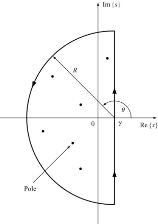
f(x) = 1 2πi
γ+i∞
γ−i∞
F(s)esxds. (17)
Here the real number γ must be chosen such that all the poles of the integrand lie to the left of the line s=γ in the complex s-plane. This integral is to be interpreted as the limit as R→ ∞ of a contour integral around the contour shown in Figure 2. This is called the Bromwich contour after the Cambridge mathematician T.J.I’A. Bromwich who introduced it at the beginning of the last century.
Example: To illustrate the application of the Laplace inversion integral it will suffice to consider findingf(x) =L−1 {1/√s}.
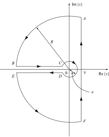
The function 1√s has a branch point at the origin, so the Bromwich contour must be modified to make the function single valued inside the contour. We will use the contour shown in Figure 3, where the branch point is enclosed in a small circle about the origin while the complexs-plane is cut along the negative real axis to make the function single valued inside the contour.
Let CR1 denote the large circular arc and CR2 denote the small circle around the origin.
Then on CR1 s=γ+Reiθfor π2 ≤θ≤ 32π, and for subsequent use we now set θ=π2 +φ, so
s=γ+iReiφwith 0≤φ≤π<