As a programmer, your bookshelf is probably overflowing with books that did nothing to change the way you program . . . or think about programming.
You’re going to need a completely different shelf for this book.
While discussing caching techniques in Chapter 3, Mark Jason Dominus points out how a large enough increase in power can change the fundamental way you think about a technology. And that’s precisely what this entire book does for Perl.
It raids the deepest vaults and highest towers of Computer Science, and transforms the many arcane treasures it finds—recursion, iterators, filters, memoization, partitioning, numerical methods, higher-order functions, currying, cutsorting, grammar-based parsing, lazy evaluation, and constraint programming—into powerful and practical tools for real-world programming tasks: file system interactions, HTML processing, database access, web spidering, typesetting, mail processing, home finance, text outlining, and diagram generation.
Along the way it also scatters smaller (but equally invaluable) gems, like the elegant explanation of the difference between “scope” and “duration” in Chapter 3, or the careful exploration of how best to return error flags in Chapter 4. It even has practical tips for Perl evangelists.
Dominus presents even the most complex ideas in simple, comprehensible ways, but never compromises on the precision and attention to detail for which he is so widely and justly admired.
His writing is—as always—lucid, eloquent, witty, and compelling.
Aptly named, this truly /is/ a Perl book of a higher order, and essential reading for every serious Perl programmer.
-
Mark Jason Dominus
AMSTERDAM • BOSTON • HEIDELBERG • LONDON NEW YORK • OXFORD • PARIS • SAN DIEGO SAN FRANCISCO • SINGAPORE • SYDNEY • TOKYO
Publishing Services Manager Simon Crump
Assistant Editor Richard Camp
Cover Design Yvo Riezebos Design
Cover Illustration Yvo Riezebos Design
Composition Cepha Imaging Pvt. Ltd.
Technical Illustration Dartmouth Publishing, Inc.
Copyeditor Eileen Kramer
Proofreader Deborah Prato
Interior Printer The Maple-Vail Book Manufacturing Group
Cover Printer Phoenix Color
Morgan Kaufmann Publishers is an imprint of Elsevier. 500 Sansome Street, Suite 400, San Francisco, CA 94111
This book is printed on acid-free paper.
© 2005 by Elsevier Inc. All rights reserved.
Designations used by companies to distinguish their products are often claimed as trademarks or registered trademarks. In all instances in which Morgan Kaufmann Publishers is aware of a claim, the product names appear in initial capital or all capital letters. Readers, however, should contact the appropriate companies for more complete information regarding trademarks and registration.
No part of this publication may be reproduced, stored in a retrieval system, or transmitted in any form or by any means—electronic, mechanical, photocopying, scanning, or otherwise—without prior written permission of the publisher.
Permissions may be sought directly from Elsevier’s Science & Technology Rights Department in Oxford, UK: phone: (+44) 1865 843830, fax: (+44) 1865 853333, e-mail:[email protected]. You may also complete your request on-line via the Elsevier homepage (http://elsevier.com) by selecting
“Customer Support” and then “Obtaining Permissions.”
Library of Congress Cataloging-in-Publication Data Application submitted
ISBN: 1-55860-701-3
For information on all Morgan Kaufmann publications, visit our Web site at www.mkp.com or www.books.elsevier.com
Printed in the United States of America
Preface. . . xv
Recursion and Callbacks. . . 1
1.1 . . . 1
1.2 . . . 3
1.2.1 Why Private Variables Are Important. . . 5
1.3 . . . 6
1.4 . . . 12
1.5 . . . 16
1.6 - . . . 25
1.7 . . . 26
1.7.1 More Flexible Selection. . . 32
1.8 . . . 33
1.8.1 Fibonacci Numbers. . . 33
1.8.2 Partitioning. . . 35
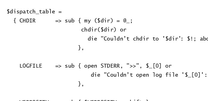
Dispatch Tables. . . 41
2.1 . . . 41
2.1.1 Table-Driven Configuration . . . 43
2.1.2 Advantages of Dispatch Tables. . . 45
2.1.3 Dispatch Table Strategies. . . 49
2.1.4 Default Actions. . . 52
2.2 . . . 54
2.2.1 HTML Processing Revisited. . . 59
Caching and Memoization. . . 63
3.1 . . . 65
3.2 . . . 66
3.2.1 Static Variables. . . 67
3.3 . . . 68
3.4 . . . 69
3.5 . . . 70
3.5.1 Scope and Duration. . . 71
Scope. . . 72
Duration. . . 73
3.5.2 Lexical Closure. . . 76
3.5.3 Memoization Again. . . 79
3.6 . . . 80
3.6.1 Functions Whose Return Values Do Not Depend on Their Arguments. . . 80
3.6.2 Functions with Side Effects. . . 80
3.6.3 Functions That Return References. . . 81
3.6.4 A Memoized Clock?. . . 82
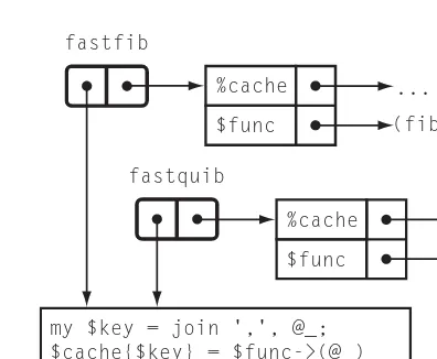
3.6.5 Very Fast Functions. . . 83
3.7 . . . 84
3.7.1 More Applications of User-Supplied Key Generators. . . 89
3.7.2 Inlined Cache Manager with Argument Normalizer. . . 90
3.7.3 Functions with Reference Arguments. . . 93
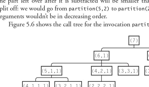
3.7.4 Partitioning. . . 93
3.7.5 Custom Key Generation for Impure Functions. . . 94
3.8 . . . 96
3.8.1 Memoization of Object Methods. . . 99
3.9 . . . 100
3.10 . . . 101
3.11 . . . 108
3.12 . . . 109
3.12.1 Profiling and Performance Analysis. . . 110
3.12.2 Automatic Profiling. . . 111
3.12.3 Hooks. . . 113
Iterators. . . 115
4.1 . . . 115
4.1.1 Filehandles Are Iterators. . . 115
4.1.2 Iterators Are Objects. . . 117
4.1.3 Other Common Examples of Iterators. . . 118
4.2 . . . 119
4.2.1 A Trivial Iterator:upto(). . . 121
Syntactic Sugar for Manufacturing Iterators. . . 122
4.2.2 dir_walk(). . . 123
4.3 . . . 126
4.3.1 Permutations. . . 128
4.3.2 Genomic Sequence Generator. . . 135
4.3.3 Filehandle Iterators. . . 139
4.3.4 A Flat-File Database. . . 140
Improved Database. . . 144
4.3.5 Searching Databases Backwards. . . 148
A Query Package That Transforms Iterators. . . 150
An Iterator That Reads Files Backwards. . . 152
Putting It Together. . . 152
4.3.6 Random Number Generation. . . 153
4.4 . . . 157
4.4.1 imap(). . . 158
4.4.2 igrep(). . . 160
4.4.3 list_iterator(). . . 161
4.4.4 append(). . . 162
4.5 . . . 163
4.5.1 Avoiding the Problem. . . 164
4.5.2 Alternativeundefs. . . 166
4.5.3 Rewriting Utilities. . . 169
4.5.4 Iterators That Return Multiple Values. . . 170
4.5.5 Explicit Exhaustion Function. . . 171
4.5.6 Four-Operation Iterators. . . 173
4.5.7 Iterator Methods. . . 176
4.6 . . . 177
4.6.1 Usingforeachto Loop Over More Than One Array. . . 177
4.6.2 An Iterator with aneach-Like Interface. . . 182
4.6.3 Tied Variable Interfaces. . . 184
Summary oftie. . . 184
Tied Scalars. . . 185
Tied Filehandles. . . 186
4.7 : . . . 187
4.7.1 Pursuing Only Interesting Links . . . 190
4.7.2 Referring URLs. . . 192
4.7.3 robots.txt. . . 197
4.7.4 Summary. . . 200
From Recursion to Iterators. . . 203
5.1 . . . 204
5.1.2 Optimizations. . . 209
5.1.3 Variations. . . 212
5.2 . . . 215
5.3 . . . 225
5.4 . . . 229
5.4.1 Tail-Call Elimination. . . 229
Someone Else’s Problem. . . 234
5.4.2 Creating Tail Calls. . . 239
5.4.3 Explicit Stacks. . . 242
Eliminating Recursion Fromfib(). . . 243
Infinite Streams. . . 255
6.1 . . . 256
6.2 . . . 257
6.2.1 A Trivial Stream:upto(). . . 259
6.2.2 Utilities for Streams. . . 260
6.3 . . . 263
6.3.1 Memoizing Streams. . . 265
6.4 . . . 269
6.5 . . . 272
6.5.1 Generating Strings in Order. . . 283
6.5.2 Regex Matching. . . 286
6.5.3 Cutsorting. . . 288
Log Files. . . 293
6.6 - . . . 300
6.6.1 Approximation Streams. . . 304
6.6.2 Derivatives. . . 305
6.6.3 The Tortoise and the Hare. . . 308
6.6.4 Finance. . . 310
6.7 . . . 313
6.7.1 Derivatives. . . 319
6.7.2 Other Functions. . . 320
6.7.3 Symbolic Computation. . . 320
Higher-Order Functions and Currying. . . 325
7.1 . . . 325
7.2 - . . . 333
7.2.1 Automatic Currying. . . 335
7.2.2 Prototypes. . . 337
7.2.3 More Currying. . . 340
7.2.4 Yet More Currying. . . 342
7.3 reduce()combine(). . . 343
7.3.1 Boolean Operators. . . 348
7.4 . . . 351
7.4.1 Operator Overloading. . . 356
Parsing. . . 359
8.1 . . . 359
8.1.1 Emulating the<>Operator. . . 360
8.1.2 Lexers More Generally. . . 365
8.1.3 Chained Lexers. . . 368
8.1.4 Peeking. . . 374
8.2 . . . 376
8.2.1 Grammars. . . 376
8.2.2 Parsing Grammars. . . 380
8.3 - . . . 384
8.3.1 Very Simple Parsers. . . 384
8.3.2 Parser Operators. . . 386
8.3.3 Compound Operators. . . 388
8.4 . . . 390
8.4.1 A Calculator. . . 400
8.4.2 Left Recursion. . . 400
8.4.3 A Variation onstar(). . . 408
8.4.4 Generic-Operator Parsers. . . 412
8.4.5 Debugging. . . 415
8.4.6 The Finished Calculator. . . 424
8.4.7 Error Diagnosis and Recovery. . . 427
Error-Recovery Parsers. . . 427
Exceptions. . . 430
8.4.8 Big Numbers. . . 435
8.5 . . . 435
8.6 . . . 440
8.7 - . . . 448
8.7.1 The Lexer. . . 448
8.7.2 The Parser. . . 451
8.8 . . . 456
8.8.1 Continuations. . . 457
8.8.2 Parse Streams. . . 461
Declarative Programming. . . 471
9.1 . . . 472
9.2 . . . 472
9.2.1 Implementing a Local Propagation Network. . . 475
9.2.2 Problems with Local Propagation. . . 487
9.3 . . . 488
9.4 linogram: . . . 490
9.4.1 Equations. . . 500
ref($base) || $base. . . 501
Solving Equations. . . 502
Constraints. . . 512
9.4.2 Values. . . 514
Constant Values. . . 516
Tuple Values. . . 518
Feature Values. . . 520
Intrinsic Constraints. . . 521
Synthetic Constraints. . . 522
Feature-Value Methods. . . 527
9.4.3 Feature Types. . . 530
Scalar Types. . . 531
TypeMethods. . . 532
9.4.4 The Parser. . . 539
Parser Extensions. . . 541
%TYPES. . . 542
Programs. . . 543
Definitions. . . 543
Declarations. . . 545
Expressions. . . 554
9.4.5 Missing Features. . . 560
9.5 . . . 563
Index. . . 565
A well-known saying in the programming racket is that a good Fortran pro-grammer can write Fortran programs in any language. The sad truth, though, is that Fortran programmers write Fortran programs in any language whether they mean to or not. Similarly, we, as Perl programmers, have been writing C programs in Perl whether we meant to or not. This is a shame, because Perl is a much more expressive language than C. We could be doing a lot better, using Perl in ways undreamt of by C programmers, but we’re not.
How did this happen? Perl was originally designed as a replacement for C on the one hand and Unix scripting languages like Bourne Shell and awkon
the other. Perl’s first major proponents were Unix system administrators, people familiar with C and with Unix scripting languages; they naturally tended to write Perl programs that resembled C andawkprograms. Perl’s inventor, Larry Wall,
came from this sysadmin community, as did Randal Schwartz, his coauthor on Programming Perl, the first and still the most important Perl reference work. Other important early contributors include Tom Christiansen, also a C-and-Unix expert from way back. Even when Perl programmers didn’t come from the Unix sysadmin community, they were trained by people who did, or by people who were trained by people who did.
Around 1993 I started reading books about Lisp, and I discovered something important: Perl is much more like Lisp than it is like C. If you pick up a good book about Lisp, there will be a section that describes Lisp’s good features. For example, the bookParadigms of Artificial Intelligence Programming, by Peter Norvig, includes a section titledWhat Makes Lisp Different?that describes seven features of Lisp. Perl shares six of these features; C shares none of them. These are big, important features, features like first-class functions, dynamic access to the symbol table, and automatic storage management. Lisp programmers have been using these features since 1957. They know a lot about how to use these language features in powerful ways. If Perl programmers can find out the things that Lisp programmers already know, they will learn a lot of things that will make their Perl programming jobs easier.
This is easier said than done. Hardly anyone wants to listen to Lisp pro-grammers. Perl folks have a deep suspicion of Lisp, as demonstrated by Larry Wall’s famous remark that Lisp has all the visual appeal of oatmeal with fingernail
clippings mixed in. Lisp programmers go around making funny noises like ‘cons’ and ‘cooder,’ and they talk about things like the PC loser-ing problem, whatever that is. They believe that Lisp is better than other programming languages, and they say so, which is irritating. But now it is all okay, because now you do not have to listen to the Lisp folks. You can listen to me instead. I will make sooth-ing noises about hashes and stashes and globs, and talk about the familiar and comforting soft reference and variable suicide problems. Instead of telling you how wonderful Lisp is, I will tell you how wonderful Perl is, and at the end you will not have to know any Lisp, but you will know a lot more about Perl.
Then you can stop writing C programs in Perl. I think that you will find it to be a nice change. Perl is much better at being Perl than it is at being a slow version of C. You will be surprised at what you can get done when you write Perl programs instead of C.
All the code examples in this book are available from my web site at:
http://perl.plover.com/hop/
When the notation in the margin is labeled with the tag some-example, the
code may be downloaded from:
http://perl.plover.com/hop/Examples/some-example
The web site will also carry the complete text, an errata listing, and other items of interest. Should you wish to send me email about the book, please send your message [email protected].
This book was a long time in coming, and Tim went through three assistants while I was working on it. All these people were helpful and competent, so my thanks to Brenda Modliszewksi, Stacie Pierce, and Richard Camp. “Competent” may sound faint, but I consider it the highest praise.
Many thanks to Troy Lilly and Simon Crump, the production managers, who were not only competent but also fun to work with.
Shortly before the book went into production, I started writing tests for the example code. I realized with horror that hardly any of the programs worked properly. There were numerous small errors (and some not so small), inconsis-tencies between the code and the output, typos, and so on. Thanks to the heroic eleventh-hour efforts of Robert Spier, I think most of these errors have been caught. Robert was not only unfailingly competent, helpful, and productive, but also unfailingly cheerful, too. If any of the example programs in this book work as they should, you can thank Robert. (If they don’t, you should blame me, not Robert.) Robert was also responsible for naming the MOD document preparation system that I used to prepare the manuscript.
The contributions of my wife, Lorrie Kim, are too large and pervasive to note individually. It is to her that this book is dedicated.
A large number of other people contributed to this book, but many of them were not aware of it at the time. I was fortunate to have a series of excellent teachers, whose patience I must sometimes have tried terribly. Thanks to Mark Foster, Patrick X. Gallagher, Joan Livingston, Cal Lobel (who first taught me to program), Harry McLaughlin, David A. J. Meyer, Bruce Piper, Ronnie Rabassa, Michael Tempel, and Johan Tysk. Mark Foster also arrived from nowhere in the nick of time to suggest the title for this book just when I thought all was lost.
This book was directly inspired by two earlier books: ML for the Working Programmer, by Lawrence Paulson, andStructure and Interpretation of Computer Programs, by Harold Abelson and Gerald Jay Sussman. Other important influ-ences wereIntroduction to Functional Programming, by Richard Bird and Philip Wadler, andParadigms of Artificial Intelligence Programming, by Peter Norvig.
The official technical reviewers had a less rewarding job than they might have on other projects. This book took a long time to write, and although I wanted to have long conversations with the reviewers about every little thing, I was afraid that if I did that, I would never ever finish. So I rarely corresponded with the reviewers, and they probably thought that I was just filing their suggestions in the shredder. But I wasn’t; I pored over all their comments with the utmost care, and agonized over most of them. My thanks to the reviewers: Sean Burke, Damian Conway, Kevin Lenzo, Peter Norvig, Dan Schmidt, Kragen Sitaker, Michael Scott, and Adam Turoff.
helpful, and I’d recommend the practice to anyone else. The six hundred and fifty wonderful members of my mailing list are too numerous to list here. All were helpful and supportive, and the book is much better for their input. A few stand out as having contributed a particularly large amount of concrete mate-rial: Roland Young, Damien Warman, David “Novalis” Turner, Iain “Spoon” Truskett, Steve Tolkin, Ben Tilly, Rob Svirskas, Roses Longin Odounga, Luc St. Louis, Jeff Mitchell, Steffen Müller, Abhijit Menon-Sen, Walt Mankowski, Wolfgang Laun, Paul Kulchenko, Daniel Koo, Andy Lester, David Landgren, Robin Houston, Torsten Hofmann, Douglas Hunter, Francesc Guasch, Ken-neth Graves, Jeff Goff, Michael Fischer, Simon Cozens, David Combs, Stas Bekman, Greg Bacon, Darius Bacon, and Peter Allen. My apologies to the many many helpful contributors whom I have deliberately omitted from this list in the interests of space, and even more so to the several especially helpful contributors whom I have accidentally omitted.
Before I started writing, I received valuable advice about choosing a publisher from Philip Greenspun, Brian Kernighan, and Adam Turoff. Damian Conway and Abigail gave me helpful advice and criticism about my proposal.
Sean Burke recorded my Ivory Tower talk and cut CDs and sent them to me and who supplied RTF-related consulting at the last minute. He also sent me periodic mail to remind me how wonderful my book was, which often arrived at times when I wasn’t so sure.
Several specific ideas in Chapter 4 were suggested by other people. Meng Wong suggested the clever and apt “odometer” metaphor. Randal Schwartz helped me with the “append” function. Eric Roode suggested the multiple list iterator.
When I needed to read out-of-print books by Paul Graham, A. E. Sundstrom lent them to me. When I needed a copy of volume 2 ofThe Art of Computer Programming, Hildo Biersma and Morgan Stanley bought it for me. When I needed money, B. B. King lent me some. Thanks to all of you.
The constraint system drawing program of Chapter 9 was a big project, and I was stuck on it for a long time. Without the timely assistance of Wm Leler, I might still be stuck.
Tom Christiansen, Jon Orwant, and Nat Torkington played essential and irreplaceable roles in integrating me into the Perl community.
1
The first “advanced” technique we’ll see is recursion. Recursion is a method of solving a problem by reducing it to a simpler problem of the same type.
Unlike most of the techniques in this book, recursion is already well known and widely understood. But it will underlie several of the later techniques, and so we need to have a good understanding of its fine points.
1.1
Until the release of Perl 5.6.0, there was no good way to generate a binary numeral in Perl. Starting in 5.6.0, you can usesprintf("%b", $num), but before that the
question of how to do this was Frequently Asked.
Any whole number has the form 2k +b, where k is some smaller whole number andbis either 0 or 1.bis the final bit of the binary expansion. It’s easy to see whether this final bit is 0 or 1; just look to see whether the input number is even or odd. The rest of the number is 2k, whose binary expansion is the same as that ofk, but shifted left one place. For example, consider the number 37=2·18+1; herekis 18 andbis 1, so the binary expansion of 37 (100101) is the same as that of 18 (10010), but with an extra 1 on the end.
How did I compute the expansion for 37? It is an odd number, so the final bit must be 1; the rest of the expansion will be the same as the expansion of 18. How can I compute the expansion of 18? 18 is even, so its final bit is 0, and the rest of the expansion is the same as the expansion of 9. What is the binary expansion for 9? 9 is odd, so its final bit is 1, and the rest of its binary expansion is
the same as the binary expansion of 4. We can continue in this way, until finally we ask about the binary expansion of 1, which of course is 1.
This procedure will work for any number. To compute the binary expansion of a numbernwe proceed as follows:
1. Ifnis 1, its binary expansion is 1, and we may ignore the rest of the procedure. Similarly, ifnis 0, the expansion is simply 0. Otherwise:
2. Computekandbso thatn =2k +bandb =0 or 1. To do this, simply dividenby 2;kis the quotient, andbis the remainder, 0 ifnwas even, and 1 ifnwas odd.
3. Compute the binary expansion of k, using this same method. Call the resultE.
4. The binary expansion fornisEb.
Let’s build a function calledbinary()that calculates the expansion. Here is the
preamble, and step 1:
sub binary {
C O D E L I B R A RY
binary my ($n) = @_;
return $n if $n == 0 || $n == 1;
Here is step 2:
my $k = int($n/2); my $b = $n % 2;
For the third step, we need to compute the binary expansion of k. How can we do that? It’s easy, because we have a handy function for computing binary expansions, called binary()— or we will once we’ve finished writing it. We’ll
callbinary()withkas its argument:
my $E = binary($k);
Now the final step is a string concatenation:
return $E . $b; }
The essential technique here was to reduce the problem to a simpler case. We were supposed to find the binary expansion of a numbern; we discovered that this binary expansion was the concatenation of the binary expansion of a smaller numberkand a single bitb. Then to solve the simpler case of the same problem, we used the functionbinary()in its own definition. When we invoke binary()with some number as an argument, it needs to computebinary()for
a different, smaller argument, which in turn computes binary() for an even
smaller argument. Eventually, the argument becomes 1, andbinary()computes
the trivial binary representation of 1 directly.
This final step, called thebase caseof the recursion, is important. If we don’t consider it, our function might never terminate. If, in the definition ofbinary(),
we had omitted the line:
return $n if $n == 0 || $n == 1;
thenbinary()would have computed forever, and would never have produced
an answer for any argument.
1.2
Suppose you have a list of n different items. For concreteness, we’ll suppose that these items are letters of the alphabet. How many different orders are there for such a list? Obviously, the answer depends on n, so it is a function ofn. This function is called thefactorial function. The factorial ofnis the number of different orders for a list ofndifferent items. Mathematicians usually write it as a postfix (!) mark, so that the factorial ofnisn!. They also call the different orders permutations.
Let’s compute some factorials. Evidently, there’s only one way to order a list of one item, so 1!=1. There are two permutations of a list of two items:A-B
andB-A, so 2!=2. A little pencil work will reveal that there are six permutations
of three items:
C AB C BA A C B B C A AB C BA C
for the two-item list we start with:ABandBA. In each case, we have three choices
about where to put theC: at the beginning, in the middle, or at the end. There
are 2·3 = 6 ways to make the choices together, and since each choice leads to a different list of three items, there must be six such lists. The preceding left column shows all the lists we got by inserting theCintoAB, and the right column
shows the lists we got by inserting theCintoBA, so the display is complete.
Similarly, if we want to know how many permutations there are of four items, we can figure it out the same way. There are six different lists of three items, and there are four positions where we could insert the fourth item into each of the lists, for a total of 6·4=24 total orders:
D ABC D ACB D BAC D BCA D CAB D CBA A D BC A D CB B D AC B D CA C D AB C D BA AB D C AC D B BA D C BC D A CA D B CB D A ABC D ACB D BAC D BCA D CAB D CBA D
Now we’ll write a function to compute, for anyn, how many permutations there are of a list ofnelements.
We’ve just seen that if we know the number of possible permutations of n−1 things, we can compute the number of permutations ofnthings. To make a list of nthings, we take one of the (n −1)! lists ofn− 1 things and insert thenth thing into one of thenavailable positions in the list. Therefore, the total number of permutations ofnitems is (n−1)! ·n:
sub factorial { my ($n) = @_;
return factorial($n-1) * $n; }
Oops, this function is broken; it never produces a result for any input, because we left out the termination condition. To computefactorial(2), it first tries
to computefactorial(1). To computefactorial(1), it first tries to compute factorial(0). To computefactorial(0), it first tries to computefactorial(-1).
This process continues forever. We can fix it by telling the function explicitly what 0! is so that when it gets to 0 it doesn’t need to make a recursive call:
sub factorial {
C O D E L I B R A RY
factorial my ($n) = @_;
return 1 if $n == 0;
Now the function works properly.
It may not be immediately apparent why the factorial of 0 is 1. Let’s return to the definition.factorial($n)is the number of different orders of a given list of $nelements.factorial(2)is 2, because there are two ways to order a list of two
elements:('A', 'B')and('B', 'A').factorial(1)is 1, because there is only
one way to order a list of one element:('A').factorial(0)is 1, because there is
only one way to order a list of zero elements:(). Sometimes people are tempted
to argue that 0! should be 0, but the example of()shows clearly that it isn’t.
Getting the base case right is vitally important in recursive functions, because if you get it wrong, it will throw off all the other results from the function. If we were to erroneously replacereturn 1in the preceding function withreturn 0,
it would no longer be a function for computing factorials; instead, it would be a function for computing zero.
1.2.1
Why Private Variables Are Important
Let’s spend a little while looking at what happens if we leave out the my. The
following version offactorial()is identical to the previous version, except that
it is missing themydeclaration on$n:
sub factorial { C O D E L I B R A RY factorial-broken
($n) = @_;
return 1 if $n == 0;
return factorial($n-1) * $n; }
Now$nis a global variable, because all Perl variables are global unless they are
declared with my. This means that even though several copies offactorial()
might be executing simultaneously, they are all using the same global variable$n.
What effect does this have on the function’s behavior?
Let’s consider what happens when we callfactorial(1). Initially,$nis set to
1, and the test on the second line fails, so the function makes a recursive call to
factorial(0). The invocation offactorial(1)waits around for the new function
call to complete. Whenfactorial(0)is entered,$nis set to 0. This time the test
on the second line is true, and the function returns immediately, yielding 1. The invocation of factorial(1) that was waiting for the answer to factorial(0)can now continue; the result fromfactorial(0)is 1.factorial(1)
takes this 1, multiplies it by the value of$n, and returns the result. But$nis now
0, becausefactorial(0)set it to 0, so the result is 1·0 = 0. This is the final,
Similarly, factorial(2) returns 0 instead of 2, factorial(3) returns 0
instead of 6, and so on.
In order to work properly, each invocation offactorial()needs to have its
own private copy of$nthat the other invocations won’t interfere with, and that’s
exactly whatmydoes. Each timefactorial()is invoked, a new variable is created
for that invocation to use as its$n.
Other languages that support recursive functions all have variables that work something like Perl’smyvariables, where a new one is created each time the
func-tion is invoked. For example, in C, variables declared inside funcfunc-tions have this behavior by default, unless declared otherwise. (In C, such variables are called autovariables, because they are automatically allocated and deallocated.) Using global variables or some other kind of storage that isn’t allocated for each invo-cation of a function usually makes it impossible to call that function recursively; such a function is callednon-reentrant. Non-reentrant functions were once quite common in the days when people used languages like Fortran (which didn’t sup-port recursion until 1990) and became less common as languages with private variables, such as C, became popular.
1.3
Both our examples so far have not actually required recursion; they could both be rewritten as simple loops.
This sort of rewriting is always possible, because after all, the machine lan-guage in your computer probably doesn’t support recursion, so in some sense it must be inessential. For the factorial function, the rewriting is easy, but this isn’t always so. Here’s an example. It’s a puzzle that was first proposed by Edouard Lucas in 1883, called the Tower of Hanoi.
The puzzle has three pegs, calledA,B, andC. On pegAis a tower of disks
of graduated sizes, with the largest on the bottom and the smallest on the top (see Figure 1.1).
The puzzle is to move the entire tower fromAtoC, subject to the following
restrictions: you may move only one disk at a time, and no disk may ever rest atop a smaller disk. The number of disks varies depending on who is posing the problem, but it is traditionally 64. We will try to solve the problem in the general case, forndisks.
Let’s consider the largest of the ndisks, which is the one on the bottom. We’ll call this disk “the Big Disk.” The Big Disk starts on pegA, and we want it
to end on pegC. If any other disks are on pegA, they are on top of the Big Disk,
so we will not be able to move it. If any other disks are on pegC, we will not be
. The initial configuration of the Tower of Hanoi.
. An intermediate stage of the Tower of Hanoi.
we want to move the Big Disk fromAtoC, all the other disks must be heaped
up on pegB, in size order, with the smallest one on top (see Figure 1.2).
This means that to solve this problem, we have a subgoal: we have to move the entire tower of disks, except for the Big Disk, fromAtoB. Only then we
can transfer the Big Disk fromAtoC. After we’ve done that, we will be able to
move the rest of the tower fromBtoC; this is another subgoal.
Fortunately, when we move the smaller tower, we can ignore the Big Disk; it will never get in our way no matter where it is. This means that we can apply the same logic to moving the smaller tower. At the bottom of the smaller tower is a large disk; we will move the rest of the tower out of the way, move this bottom disk to the right place, and then move the rest of the smaller tower on top of it. How do we move the rest of the smaller tower? The same way.
would be illegal) and we know that we can always move it wherever we like; it’s the smallest, so it is impossible to put it atop anything smaller.
Our strategy for moving the original tower looks like this: To move a tower ofndisks from the start peg to the end peg,
1. If the “tower” is actually only one disk high, just move it. Otherwise: 2. Move all the disks except for diskn(the Big Disk) from the start peg to the
extra peg, using this method.
3. Move diskn(the Big Disk) from the start peg to the end peg.
4. Move all the other disks from the extra peg to the end peg, using this method.
It’s easy to translate this into code:
# hanoi(N, start, end, extra)
C O D E L I B R A RY
hanoi # Solve Tower of Hanoi problem for a tower of N disks,
# of which the largest is disk #N. Move the entire tower from # peg 'start' to peg 'end', using peg 'extra' as a work space sub hanoi {
my ($n, $start, $end, $extra) = @_; if ($n == 1) {
print "Move disk #1 from $start to $end.\n"; # Step 1 } else {
hanoi($n-1, $start, $extra, $end); # Step 2 print "Move disk #$n from $start to $end.\n"; # Step 3 hanoi($n-1, $extra, $end, $start); # Step 4 }
}
This function prints a series of instructions for how to move the tower. For example, to ask it for instructions for moving a tower of three disks, we call it like this:
hanoi(3, 'A', 'C', 'B');
Its output is:
Move disk #1 from B to A. Move disk #2 from B to C. Move disk #1 from A to C.
If we wanted a graphic display of moving disks instead of a simple printout of instructions, we could replace theprintstatements with something fancier.
But we can make the software more flexible almost for free by parametrizing the output behavior. Instead of having aprintstatement hardwired in,hanoi()
will accept an extra argument that is a function that will be called each time
hanoi()wants to move a disk. This function will print an instruction, or update
a graphical display, or do whatever else we want. The function will be passed the number of the disk, and the source and destination pegs. The code is almost exactly the same:
sub hanoi {
my ($n, $start, $end, $extra, $move_disk) = @_;
if ($n == 1) {
$move_disk->(1, $start, $end);
} else {
hanoi($n-1, $start, $extra, $end, $move_disk);
$move_disk->($n, $start, $end);
hanoi($n-1, $extra, $end, $start, $move_disk); }
}
To get the behavior of the original version, we now invokehanoi()like this:
sub print_instruction {
my ($disk, $start, $end) = @_;
print "Move disk #$disk from $start to $end.\n"; }
hanoi(3, 'A', 'C', 'B', \&print_instruction);
The\&print_instructionexpression generates acode reference, which is a scalar
value that represents the function. You can store the code reference in a scalar variable just like any other scalar, or pass it as an argument just like any other scalar, and you can also use the reference to invoke the function that it represents. To do that, you write:
This invokes the function with the specified arguments.1 Code references are
often referred to ascoderefs.
The coderef argument tohanoi()is called acallback, because it is a function
supplied by the caller of hanoi() that will be “called back” to when hanoi()
needs help. We sometimes also say that the $move_disk argument of hanoi()
is ahook, because it provides a place where additional functionality may easily be hung.
Now that we have a generic version ofhanoi(), we can test the algorithm
by passing in a$move_diskfunction that keeps track of where the disks are and
checks to make sure we aren’t doing anything illegal:
@position = ('', ('A') x 3); # Disks are all initially on peg A
C O D E L I B R A RY check-move
sub check_move { my $i;
my ($disk, $start, $end) = @_;
Thecheck_move()function maintains an array,@position, that records the
cur-rent position of every disk. Initially, every disk is on pegA. Here we assume
that there are only three disks, so we set $position[1], $position[2], and $position[3] to "A". $position[0] is a dummy element that is never used
because there is no disk 0. Each time the mainhanoi()function wants to move
a disk, it callscheck_move().
if ($disk < 1 || $disk > $#position) {
die "Bad disk number $disk. Should be 1..$#position.\n"; }
This is a trivial check to make sure thathanoi()doesn’t try to move a nonexistent
disk.
unless ($position[$disk] eq $start) {
die "Tried to move disk $disk from $start, but it is on peg $position[$disk].\n"; }
Here the function checks to make sure thathanoi()is not trying to move a disk
from a peg where it does not reside. If the start peg does not matchcheck_move()’s
notion of the current position of the disk, the function signals an error.
for $i (1 .. $disk-1) {
if ($position[$i] eq $start) {
die "Can't move disk $disk from $start because $i is on top of it.\n"; } elsif ($position[$i] eq $end) {
die "Can't move disk $disk to $end because $i is already there.\n"; }
}
This is the really interesting check. The function loops over all the disks that are smaller than the onehanoi()is trying to move, and makes sure that the smaller
disks aren’t in the way. The firstifbranch makes sure that each smaller disk is
not on top of the onehanoi()wants to move, and the second branch makes sure
thathanoi()is not trying to move the current disk onto the smaller disk.
print "Moving disk $disk from $start to $end.\n"; $position[$disk] = $end;
}
Finally, the function has determined that there is nothing wrong with the move, so it prints out a message as before, and adjusts the@positionarray to reflect the
new position of the disk. Running:
hanoi(3, 'A', 'C', 'B', \&check_move);
yields the same output as before, and no errors —hanoi()is not doing anything
illegal.
1.4
The examples we’ve seen give the flavor of what a recursive procedure looks like, but they miss an important point. In introducing the Tower of Hanoi problem, I said that recursion is useful when you want to solve a problem that can be reduced to simpler cases of the same problem. But it might not be clear that such problems are common.
Most recursive functions are built to deal with recursive data structures. A recursive data structure is one like a list, tree, or heap that is defined in terms of simpler instances of the same data structure. The most familiar example is probably a file system directory structure. A file is either:
• a plain file, which contains some data, or • a directory, which contains a list of files
A file might be a directory, which contains a list of files, some of which might be directories, which in turn contain more lists of files, and so on. The most effective way of dealing with such a structure is with a recursive procedure. Conceptually, each call to such a procedure handles a single file. The file might be a plain file, or it might be a directory, in which case the procedure makes recursive calls to itself to handle any subfiles that the directory has. If the subfiles are themselves directories, the procedure will make more recursive calls.
Here’s an example of a function that takes the name of a directory as its argument and computes the total size of all the files contained in it, and in its subdirectories, and in their subdirectories, and so on:
sub total_size {
C O D E L I B R A RY
total-size-broken my ($top) = @_;
my $total = -s $top;
When we first call the function, it’s with an argument$top, which is the name of
the file or directory we want to examine. The first thing the function does is use the Perl-soperator to find the size of this file or directory itself. This operator
yields the size of the file, in bytes. If the file is a directory, it says how much space the directory itself takes up on the disk, apart from whatever files the directory may contain — the directory is a list of files, remember, and the list takes up some space too. If the top file is actually a directory, the function will add the sizes of its contents to a running total that it will keep in$total.
warn "Couldn’t open directory $top: $!; skipping.\n"; return $total;
}
The-foperator checks to see if the argument is a plain file; if so, the function can
return the total immediately. Otherwise, it assumes that the top file is actually a directory, and tries to open it withopendir(). If the directory can’t be opened,
the function issues a warning message and returns the total so far, which includes the size of the directory itself, but not its contents.
my $file;
while ($file = readdir DIR) {
next if $file eq '.' || $file eq '..'; $total += total_size("$top/$file"); }
The next block, thewhileloop, is the heart of the function. It reads filenames
from the directory one at a time, calls itself recursively on each one, and adds the result to the running total.
closedir DIR; return $total; }
At the end of the loop, the function closes the directory and returns the total.
In the loop, the function skips over the names.and.., which are aliases for
the directory itself and for its parent; if it didn’t do this, it would never finish, because it would try to compute the total sizes of a lot of files with names like
././././././fredanddir/../dir/../dir/../dir/fred.
This function has a gigantic bug, and in fact it doesn’t work at all. The problem is that directory handles, likeDIR, are global, and so our function is not
reentrant. The function fails for essentially the same reason that themy-less version
of factorial() failed. The first call goes ahead all right, but iftotal_size()
calls itself recursively, the second invocation will open the same dirhandleDIR.
Eventually, the second invocation will reach the end of its directory, closeDIR,
and return. When this happens, the first invocation will try to continue, find that
DIRhas been closed, and exit thewhileloop without having read all the filenames
The result is that the function, as written, looks down only the first branch of the directory tree. If the directory hierarchy has a structure like this:
Top
a b c
l j k
d e f g h i
then our function will go down thetop-a-dpath, see filesjandk, and report the total size oftop+a+d+j+k, without ever noticingb,c,e,f,g,h,i, orl.
To fix it, we need to make the directory handleDIRa private variable, like$top
and$total. Instead ofopendir DIR, $top, we’ll useopendir $dir, $top, where $diris a private variable. When the first argument toopendir is an undefined
variable,opendirwill create a new, anonymous dirhandle and store it into$dir.2
Instead of doing this:
opendir DIR, $somedir; print (readdir DIR); closedir DIR;
we can get the same effect by doing this instead:
my $dir;
opendir $dir, $somedir; print (readdir $dir); closedir $dir;
The big difference is thatDIRis a global dirhandle, and can be read or closed by
any other part of the program; the dirhandle in$diris private, and can be read
or closed only by the function that creates it, or by some other function that is explicitly passed the value of$dir.
With this new technique, we can rewrite thetotal_size()function so that
it works properly:
sub total_size { C O D E L I B R A RY total-size
my ($top) = @_; my $total = -s $top;
my $DIR;
return $total if -f $top;
unless (opendir $DIR, $top) {
warn "Couldn’t open directory $top: $!; skipping.\n"; return $total;
}
my $file;
while ($file = readdir $DIR) {
next if $file eq '.' || $file eq '..'; $total += total_size("$top/$file"); }
closedir $DIR;
return $total; }
Actually, theclosedirhere is unnecessary, because dirhandles created with this
method close automatically when the variables that contain them go out of scope. Whentotal_size()returns, its private variables are destroyed, including$DIR,
which contains the last reference to the dirhandle object we opened. Perl then destroys the dirhandle object, and in the process, closes the dirhandle. We will omit the explicitclosedirin the future.
This function still has some problems: it doesn’t handle symbolic links cor-rectly, and if a file has two names in the same directory, it gets counted twice. Also, on Unix systems, the space actually taken up by a file on disk is usually different from the length reported by-s, because disk space is allocated in blocks
1.5
Having a function that walks a directory tree is useful, and we might like to use it for all sorts of things. For example, if we want to write a recursive file lister that works like the Unixls -Rcommand, we’ll need to walk the directory tree.
We might want our function to behave more like the Unixducommand, which
prints out the total size of every subdirectory, as well as the total for all the files it found. We might want our function to search for dangling symbolic links; that is, links that point to nonexistent files. A frequently asked question in the Perl newsgroups and IRC channels is how to walk a directory tree and rename each file or perform some other operation on each file.
We could write many different functions to do these tasks, each one a little different. But the core part of each one is the recursive directory walker, and we’d like to abstract that out so that we can use it as a tool. If we can separate the walker, we can put it in a library, and then anyone who needs a directory walker can use ours.
An important change of stance occurred in the last paragraph. Starting from here, and for most of the rest of the book, we are going to take a point of view that you may not have seen before: we are no longer interested in devel-oping a complete program that we or someone else might use entirely. Instead, we are going to try to write our code so that it is useful to another program-mer who might want to re-use it in another program. Instead of writing a program, we are now writing a library or module that will be used by other programs.
One direction that we could go from here would be to show how to write auser interfacefor thetotal_size()function, which might prompt the user for
a directory name, or read a directory name from the command line or from a graphical widget, and then would display the result somehow. We are not going to do this. It is not hard to add code to prompt the user for a directory name or to read the command-line arguments. For the rest of this book, we are not going to be concerned with user interfaces; instead, we are going to look at programmer interfaces. The rest of the book will talk about “the user,” but it’s not the usual user. Instead, the user is another programmer who wants to use our code when writing their own programs. Instead of asking how we can make our entire program simple and convenient for an end-user, we will look at ways to make our functions and libraries simple and convenient for other programmers to use in their own programs.
familiar directory-walking function into every program that needs one. When we improve the directory-walking function in one program, it will be automatically improved in all our other programs as well. Over time, we’ll develop a toolkit of useful functions and libraries that will make us more productive, and we’ll have more fun programming.
But more importantly, if our functions are well designed for re-use, other programmers will be able to use them, and they will get the same benefits that we do. And being useful to other people is the reason we’re here in the first place.3
With that change of stance clearly in mind, let’s go on. We had written a function, total_size(), which contained useful functionality: it walked a
directory tree recursively. If we could cleanly separate the directory-walking part of the code from the total-size-computing part, then we might be able to re-use the directory-walking part in many other projects for many other purposes. How can we separate the two functionalities?
As in the Tower of Hanoi program, the key here is to pass an additional parameter to our function. The parameter will itself be a function that tells
total_size()what we want it to do. The code will look like this:
sub dir_walk { C O D E L I B R A RY dir-walk-simple
my ($top, $code) = @_; my $DIR;
$code->($top);
if (-d $top) { my $file;
unless (opendir $DIR, $top) {
warn "Couldn’t open directory $top: $!; skipping.\n"; return;
}
while ($file = readdir $DIR) {
next if $file eq '.' || $file eq '..'; dir_walk("$top/$file", $code);
} } }
This function, which I’ve renameddir_walk()to honor its new generality, gets
two arguments. The first,$top, is the name of the file or directory that we want
it to start searching in, as before. The second,$code, is new. It’s a coderef that
tellsdir_walkwhat we want to do for each file or directory that we discover in
the file tree. Each timedir_walk()discovers a new file or directory, it will invoke
our code with the filename as the argument.
Now whenever we meet another programmer who asks us, “How do I doX for every file in a directory tree?” we can answer, “Use thisdir_walk()function,
and give it a reference to a function that does X.” The $code argument is a
callback.
For example, to get a program that prints out a list of all the files and directories below the current directory, we can use:
sub print_dir { print $_[0], "\n"; }
dir_walk('.', \&print_dir );
This prints out something like this:
. ./a ./a/a1 ./a/a2 ./b ./b/b1 ./c ./c/c1 ./c/c2 ./c/c3 ./c/d ./c/d/d1 ./c/d/d2
(The current directory contains three subdirectories, named a, b, andc.
Sub-directoryccontains a sub-subdirectory, namedd.)
print_diris so simple that it’s a shame to have to waste time thinking of a
name for it. It would be convenient if we could simply write the function without having to write a name for it, analogous to the way we can write:
without having to name the 40 or store it in a variable. Perl does provide a syntax for this:
dir_walk('.', sub { print $_[0], "\n" } );
Thesub { ... }introduces ananonymous function; that is, a function with no
name. The value of the sub { ... }construction is a coderef that can be used
to call the function. We can store this coderef in a scalar variable or pass it as an argument to a function like any other reference. This one line does the same thing as our more verbose version with the namedprint_dirfunction.
If we want the function to print out sizes along with filenames, we need only make a small change to the coderef argument:
dir_walk('.', sub { printf "%6d %s\n", -s $_[0], $_[0] } );
4096 . 4096 ./a
261 ./a/a1 171 ./a/a2 4096 ./b
348 ./b/b1 4096 ./c
658 ./c/c1 479 ./c/c2 889 ./c/c3 4096 ./c/d
568 ./c/d/d1 889 ./c/d/d2
If we want the function to locate dangling symbolic links, it’s just as easy:
dir_walk('.', sub { print $_[0], "\n" if -l $_[0] && ! -e $_[0] });
-ltests the current file to see if it’s a symbolic link, and-etests to see if the file
that the link points at exists.
But my promises fall a little short. There’s no simple way to get the new
dir_walk()function to aggregate the sizes of all the files it sees.$codeis invoked
for only one file at a time, so it never gets a chance to aggregate. If the aggregation is sufficiently simple, we can accomplish it with a variable defined outside the callback:
dir_walk('.', sub { $TOTAL += -s $_[0] }); print "Total size is $TOTAL.\n";
There are two drawbacks to this approach. One is that the callback function must reside in the scope of the$TOTALvariable, as must any code that plans to
use$TOTAL. Often this isn’t a problem, as in this case, but if the callback were a
complicated function in a library somewhere, it might present difficulties. We’ll see a solution to this problem in Section 2.1.
The other drawback is that it works well only when the aggregation is extremely simple, as it is here. Suppose instead of accumulating a single total size, we wanted to build a hash structure of filenames and sizes, like this one:
{
'a' => {
'a1' => '261', 'a2' => '171' },
'b' => {
'b1' => '348' },
'c' => {
'c1' => '658', 'c2' => '479', 'c3' => '889', 'd' => {
'd1' => '568', 'd2' => '889' }
} }
Here the keys are file and directory names. The value for a filename is the size of the file, and the value for a directory name is a hash with keys and values that represent the contents of the directory. It may not be clear how we could adapt the simple$TOTAL-aggregating callback to produce a complex structure like
this one.
Ourdir_walkfunction is not general enough. We need it to perform some
computation involving the files it examines, such as computing their total size, and to return the result of this computation to its caller. The caller might be the main program, or it might be another invocation ofdir_walk(), which can then
How can dir_walk() know how to perform the computation? In total_size(), the addition computation was hardwired into the function. We
would likedir_walk()to be more generally useful.
What we need is to supply two functions: one for plain files and one for directories.dir_walk()will call the plain-file function when it needs to compute
its result for a plain file, and it will call the directory function when it needs to compute its result for a directory. dir_walk()won’t know anything about how
to do these computations itself; all it knows is that is should delegate the actual computing to these two functions.
Each of the two functions will get a filename argument, and will compute the value of interest, such as the size, for the file named by its argument. Since a directory is a list of files, the directory function will also receive a list of the values that were computed for each of its members; it may need these values when it computes the value for the entire directory. The directory function will know how to aggregate these values to produce a new value for the entire directory.
With this change, we’ll be able to do ourtotal_sizeoperation. The plain-file
function will simply return the size of the file it’s asked to look at. The directory function will get a directory name and a list of the sizes of each file that it contains, add them all up, and return the result. The generic framework function looks like this:
sub dir_walk { C O D E L I B R A RY dir-walk-cb my ($top, $filefunc, $dirfunc) = @_;
my $DIR;
if (-d $top) { my $file;
unless (opendir $DIR, $top) {
warn "Couldn’t open directory $code: $!; skipping.\n"; return;
}
my @results;
while ($file = readdir $DIR) {
next if $file eq '.' || $file eq '..';
push @results, dir_walk("$top/$file", $filefunc, $dirfunc);
}
return $dirfunc->($top, @results); } else {
return $filefunc->($top); }
To compute the total size of the current directory, we will use this:
sub file_size { -s $_[0] }
sub dir_size { my $dir = shift; my $total = -s $dir; my $n;
for $n (@_) { $total += $n } return $total;
}
$total_size = dir_walk('.', \&file_size, \&dir_size);
Thefile_size()function says how to compute the size of a plain file, given its
name, and thedir_size()function says how to compute the size of a directory,
given the directory name and the sizes of its contents.
If we want the program to print out the size of every subdirectory, the way theducommand does, we add one line:
sub file_size { -s $_[0] }
sub dir_size { my $dir = shift; my $total = -s $dir; my $n;
for $n (@_) { $total += $n }
printf "%6d %s\n", $total, $dir;
return $total; }
$total_size = dir_walk('.', \&file_size, \&dir_size);
This produces an output like this:
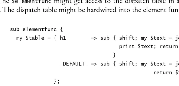
To get the function to produce the hash structure we saw earlier, we can supply the following pair of callbacks:
sub file { C O D E L I B R A RY
dir-walk-sizehash
my $file = shift;
[short($file), -s $file]; }
sub short {
my $path = shift; $path =˜ s{.*/}{}; $path;
}
The file callback returns an array with the abbreviated name of the file (no full path) and the file size. The aggregation is, as before, performed in the directory callback:
sub dir {
my ($dir, @subdirs) = @_; my %new_hash;
for (@subdirs) {
my ($subdir_name, $subdir_structure) = @$_; $new_hash{$subdir_name} = $subdir_structure; }
return [short($dir), \%new_hash]; }
The directory callback gets the name of the current directory, and a list of name– value pairs that correspond to the subfiles and subdirectories. It merges these pairs into a hash, and returns a new pair with the short name of the current directory and the newly constructed hash for the current directory.
The simpler functions that we wrote before are still easy. Here’s the recursive file lister. We use the same function for files and for directories:
sub print_filename { print $_[0], "\n" }
dir_walk('.', \&print_filename, \&print_filename);
Here’s the dangling symbolic link detector:
print "$file\n" if -l $file && ! -e $file; }
dir_walk('.', \&dangles, sub {});
We know that a directory can’t possibly be a dangling symbolic link, so our directory function is the null functionthat returns immediately without doing anything. If we had wanted, we could have avoided this oddity, and its associated function-call overhead, as follows:
sub dir_walk {
C O D E L I B R A RY
dir-walk-cb-def my ($top, $filefunc, $dirfunc) = @_;
my $DIR; if (-d $top) {
my $file;
unless (opendir $DIR, $top) {
warn "Couldn’t open directory $code: $!; skipping.\n"; return;
}
my @results;
while ($file = readdir $DIR) {
next if $file eq '.' || $file eq '..';
push @results, dir_walk("$top/$file", $filefunc, $dirfunc); }
return $dirfunc ? $dirfunc->($top, @results) : () ;
} else {
return $filefunc ? $filefunc->($top): () ;
} }
This allows us to write dir_walk('.', \&dangles) instead of dir_walk('.', \&dangles, sub {}).
As a final example, let’s use dir_walk() in a slightly different way, to
manufacture a list of all the plain files in a file tree, without printing anything:
@all_plain_files =
dir_walk('.', sub { $_[0] }, sub { shift; return @_ });
dir_walk(), and this empty list will be merged into the result list for the other
directories at the same level.
1.6
- -
Now let’s back up a moment and look at what we did. We had a useful function,
total_size(), which contained code for walking a directory structure that was
going to be useful in other applications. So we madetotal_size()more general
by pulling out all the parts that related to the computation of sizes, and replacing them with calls to arbitrary user-specified functions. The result wasdir_walk().
Now, for any program that needs to walk a directory structure and do something,
dir_walk()handles the walking part, and the argument functions handle the “do
something” part. By passing the appropriate pair of functions todir_walk(), we
can make it do whatever we want it to. We’ve gained flexibility and the chance to re-use thedir_walk()code by factoring out the useful part and parametrizing
it with two functional arguments. This is the heart of the functional style of programming.
Object-oriented (OO) programming style gets a lot more press these days. The goals of the OO style are the same as those of the functional style: we want to increase the re-usability of software components by separating them into generally useful parts.
In an OO system, we could have transformed total_size() analogously,
but the result would have looked different. We would have madetotal_size()
into an abstract base class of directory-walking objects, and these objects would have had a method,dir_walk(), which in turn would make calls to two
unde-fined virtual methods called file and directory. (In C++ jargon, these are
called pure virtual methods.) Such a class wouldn’t have been useful by itself, because thefileanddirectorymethods would be missing. To use the class, you
would create a subclass that defined thefileanddirectorymethods, and then
create objects in the subclass. These objects would all inherit the samedir_walk
method.
of the techniques will be directly applicable to object-oriented programming styles also.
1.7
I promised that recursion was useful for operating on hierarchically defined data structures, and I used the file system as an example. But it’s a slightly peculiar example of a data structure, since we normally think of data structures as being in memory, not on the disk.
What gave rise to the tree structure in the file system was the presence of directories, each of which contains a list of other files. Any domain that has items that include lists of other items will contain tree structures. An excellent example is HTML data.
HTML data is a sequence of elements and plain text. Each element has some content, which is a sequence of more elements and more plain text. This is a recursive description, analogous to the description of the file system, and the structure of an HTML document is analogous to the structure of the file system.
Elements are tagged with astart tag, which looks like this:
<font>
and a correspondingend tag, like this:
</font>
The start tag may have a set ofattribute–value pairs, in which case it might look something like this instead:
<font size=3 color="red">
The end tag is the same in any case. It never has any attribute–value pairs. In between the start and end tags can be any sequence of HTML text, including more elements, and also plain text. Here’s a simple example of an HTML document:
<h1>What Junior Said Next</h1>
<p>But I don’t <font size=3 color="red">want</font> to go to bed now!</p>
(document)
<h1> newlines <p>
What Junior Said Next But I don't <font> to go to bed now!
want
. An HTML document.
The main document has three components: the<h1>element, with its
con-tents; the<p>element, with its contents; and the blank space in between. The <p>element, in turn, has three components: the untagged text before the<font>
element; the<font>element, with its contents; and the untagged text after the <font>element. The<h1>element has one component, which is the untagged
text What Junior Said Next.
In Chapter 8, we’ll see how to build parsers for languages like HTML. In the meantime, we’ll look at a semi-standard module,HTML::TreeBuilder, which
converts an HTML document into a tree structure.
Let’s suppose that the HTML data is already in a variable, say$html. The
following code usesHTML::TreeBuilderto transform the text into an explicit tree
structure:
use HTML::TreeBuilder;
my $tree = HTML::TreeBuilder->new; $tree->ignore_ignorable_whitespace(0); $tree->parse($html);
$tree->eof();
Theignore_ignorable_whitespace()method tellsHTML::TreeBuilder that it’s
not allowed to discard certain whitespace, such as the newlines after the <h1>
element, that are normally ignorable.
Now$treerepresents the tree structure. It’s a tree of hashes; each hash is a
node in the tree and represents one element. Each hash has a _tagkey whose
value is its tag name, and a_contentkey whose value is a list of the element’s
contents, in order; each item in the_contentlist is either a string, representing
So for example, the tree node that corresponds to the<font>element in the
example looks like this:
{ _tag => "font",
_content => [ "want" ], color => "red",
size => 3, }
The tree node that corresponds to the <p>element contains the<font> node,
and looks like this:
{ _tag => "p",
_content => [ "But I don't ", { _tag => "font",
_content => [ "want" ], color => "red",
size => 3, },
" to go to bed now!", ],
}
It’s not hard to build a function that walks one of these HTML trees and “untags” all the text, stripping out the tags. For each item in a _content list, we can
recognize it as an element with the ref()function, which will yield true for
elements (which are hash references) and false for plain strings:
sub untag_html {
C O D E L I B R A RY
untag-html my ($html) = @_;
return $html unless ref $html; # It’s a plain string
my $text = '';
for my $item (@{$html->{_content}}) { $text .= untag_html($item);
}
return $text; }