CONTEXTUAL CLASSIFICATION OF POINT CLOUD DATA BY EXPLOITING
INDIVIDUAL 3D NEIGBOURHOODS
M. Weinmanna, A. Schmidtb, C. Malletc, S. Hinza, F. Rottensteinerb, B. Jutzia
a
Institute of Photogrammetry and Remote Sensing, Karlsruhe Institute of Technology (KIT) Englerstr. 7, 76131 Karlsruhe, Germany -{martin.weinmann, stefan.hinz, boris.jutzi}@kit.edu
b
Institute of Photogrammetry and GeoInformation, Leibniz Universit¨at Hannover Nienburger Str. 1, 30167 Hannover, Germany -{alena.schmidt, rottensteiner}@ipi.uni-hannover.de
cUniversit´e Paris-Est, IGN, SRIG, MATIS
73 avenue de Paris, 94160 Saint-Mand´e, France - [email protected]
Commission III, WG III/4
KEY WORDS:Lidar, Laser Scanning, Point Cloud, Features, Classification, Contextual Learning, 3D Scene Analysis, Urban
ABSTRACT:
The fully automated analysis of 3D point clouds is of great importance in photogrammetry, remote sensing and computer vision. For reliably extracting objects such as buildings, road inventory or vegetation, many approaches rely on the results of a point cloud classification, where each 3D point is assigned a respective semantic class label. Such an assignment, in turn, typically involves statistical methods for feature extraction and machine learning. Whereas the different components in the processing workflow have extensively, but separately been investigated in recent years, the respective connection by sharing the results of crucial tasks across all components has not yet been addressed. This connection not only encapsulates the interrelated issues of neighborhood selection and feature extraction, but also the issue of how to involve spatial context in the classification step. In this paper, we present a novel and generic approach for 3D scene analysis which relies on (i) individually optimized 3D neighborhoods for (ii) the extraction of distinctive geometric features and (iii) the contextual classification of point cloud data. For a labeled benchmark dataset, we demonstrate the beneficial impact of involving contextual information in the classification process and that using individual 3D neighborhoods of optimal size significantly increases the quality of the results for both pointwise and contextual classification.
1 INTRODUCTION
The fully automated analysis of 3D point clouds has become a topic of major interest in photogrammetry, remote sensing and computer vision. Recent research addresses a variety of topics such as object detection (Pu et al., 2011; Velizhev et al., 2012; Bremer et al., 2013; Serna and Marcotegui, 2014), extraction of curbstones and road markings (Zhou and Vosselman, 2012; Guan et al., 2014), urban accessibility analysis (Serna and Marcotegui, 2013), or the creation of large-scale city models (Lafarge and Mallet, 2012). A crucial task for many of these applications is point cloud classification, which aims at assigning a semantic class label to each 3D point of a given point cloud. Due to the complexity of 3D scenes caused by the irregular sampling of 3D points, varying point density and very different types of objects, point cloud classification has also become an active field of re-search, e.g. (Guo et al., 2014; Niemeyer et al., 2014; Schmidt et al., 2014; Weinmann et al., 2014; Xu et al., 2014).
Most of the approaches for point cloud classification consider the different components of the classification process (i.e. neigh-borhood selection, feature extraction and classification) indepen-dently from each other. However, it would seem desirable to connect these components by sharing the results of crucial tasks across all of them. Such a connection would not only be relevant for the interrelated problems of neighborhood selection and fea-ture extraction, but also for the question of how to involve spatial context in the classification task.
In this paper, we focus on the combination of (i) feature extrac-tion from individual 3D neighborhoods and (ii) contextual clas-sification of point cloud data. This is motivated by the fact that such a combination provides further important insights into the interrelated issues of neighborhood selection, feature extraction
and contextual classification. Using features extracted from in-dividual neighborhoods has a significantly beneficial impact on the individual classification of points (Weinmann et al., 2014). On the other hand, using contextual information might even have more influence on the classification accuracy, because it takes into account that class labels of neighboring 3D points tend to be correlated. Consequently, this paper addresses the question whether the use of features extracted from neighborhoods of in-dividual size still improves the classification accuracy when con-textual classification is applied, and whether it is beneficial to use the same neighborhood definition for contextual classification. We propose a novel and generic approach for 3D scene analy-sis which relies on individually optimized 3D neighborhoods for both feature extraction and contextual classification. Consider-ing different neighborhood definitions as the basis for feature ex-traction, we use a Conditional Random Field (CRF) (Lafferty et al., 2001) for contextual classification and compare the respective classification results with those obtained when using a Random Forest classifier (Breiman, 2001). As the unary terms of the CRF are also based on a Random Forest classifier, we can quantify the influence of the context model on the classification results.
After reflecting related work in Section 2, we explain the differ-ent compondiffer-ents of our methodology in Section 3. Subsequdiffer-ently, in Section 4, we evaluate the proposed methodology on a labeled point cloud dataset representing an urban environment and dis-cuss the derived results. Finally, in Section 5, concluding remarks and suggestions for future work are provided.
2 RELATED WORK
2.1 Fixed vs. Individual 3D Neighborhoods
In order to describe the local 3D structure at a given 3D point, the spatial arrangement of 3D points within the local neighbor-hood is typically taken into consideration. The respective local neighborhood may be defined as a spherical (Lee and Schenk, 2002) or cylindrical (Filin and Pfeifer, 2005) neighborhood with fixed radius. Alternatively, the local neighborhood can be de-fined to consist of thek∈Nnearest neighbors either on the basis
of 3D distances (Linsen and Prautzsch, 2001) or 2D distances (Niemeyer et al., 2014). The latter definition based on thek near-est neighbors offers more flexibility with respect to the absolute neighborhood size and is more adaptive to varying point density. All these neighborhood definitions, however, rely on a scale pa-rameter (i.e. either a radius ork), which is commonly selected to be identical for all 3D points and determined via heuristic or empiric knowledge on the scene. As a result, the derived scale parameter is specific for each dataset.
In order to obtain a solution taking into account that the selection of a scale parameter depends on the local 3D structure as well as the local point density, an individual neighborhood size can be determined for each 3D point. In this context, most approaches rely on a neighborhood consisting of the k nearest neighbors and thus focus on optimizing k for each individual 3D point. This optimization may for instance be based on the local sur-face variation (Pauly et al., 2003; Belton and Lichti, 2006), it-erative schemes relating neighborhood size to curvature, point density and noise of normal estimation (Mitra and Nguyen, 2003; Lalonde et al., 2005), dimensionality-based scale selection (De-mantk´e et al., 2011) or eigenentropy-based scale selection (Wein-mann et al., 2014). In particular, the latter two approaches have proven to be suitable for point cloud data acquired via mobile laser scanning, and a significant improvement of classification re-sults can be observed in comparison to the use of fixed 3D neigh-borhoods with identical scale parameter (Weinmann et al., 2014).
2.2 Single-Scale vs. Multi-Scale Features
Given a 3D point and its local neighborhood, geometric features may be derived from the spatial arrangement of all 3D points within the neighborhood. For this purpose, it has been proposed to sample geometric relations such as distances, angles and angu-lar variations between 3D points within the local neighborhood (Osada et al., 2002; Rusu et al., 2008; Blomley et al., 2014). However, the individual entries of the resulting feature vectors are hardly interpretable, and consequently, other investigations focus on deriving interpretable features. Such features may for instance be obtained by calculating the 3D structure tensor from the 3D co-ordinates of all points within the local neighborhood (Pauly et al., 2003). The eigenvalues of the 3D structure tensor may directly be applied for characterizing specific shape primitives (Jutzi and Gross, 2009). In order to obtain more intuitive features which also indicate linear, planar or volumetric structures, a set of fea-tures derived from these eigenvalues has been presented (West et al., 2004) which is nowadays commonly applied in lidar data processing. This standard feature set may be complemented by further geometric features derived from angular statistics (Munoz et al., 2009), height and local plane characteristics (Mallet et al., 2011), height characteristics and curvature properties (Schmidt et al., 2012; Schmidt et al., 2013), or basic properties of the neigh-borhood and characteristics of a 2D projection (Weinmann et al., 2013; Weinmann et al., 2014). Furthermore, the combination with full-waveform and echo-based features has been proposed (Chehata et al., 2009; Mallet et al., 2011; Niemeyer et al., 2011).
When deriving features at a single scale, one has to consider that a suitable scale (in the form of either fixed or individual 3D
neighborhoods) is required in order to obtain an appropriate de-scription of the local 3D structure. As an alternative to selecting such an appropriate scale, we may also derive features at multi-ple scales and subsequently involve a classifier in order to define which combination of scales allows the best separation of differ-ent classes (Brodu and Lague, 2012). In this context, features may even be extracted by considering different entities such as points and regions (Xiong et al., 2011; Xu et al., 2014) or by in-volving a hierarchical segmentation based on voxels, blocks and pillars (Hu et al., 2013). However, multi-scale approaches result in feature spaces of higher dimension, so that it may be advisable to use appropriate feature selection schemes in order to gain pre-dictive accuracy while at the same time reducing the extra com-putational burden in terms of both time and memory consumption (Guyon and Elisseeff, 2003).
2.3 Individual vs. Contextual Classification
Based on the derived feature vectors, classification is typically conducted in a supervised way, where the straightforward solu-tion consists of an independent classificasolu-tion of each 3D point re-lying only on its individual feature vector. The list of respective classification methods that have been used for lidar data process-ing includes classical Maximum Likelihood classifiers based on Gaussian Mixture Models (Lalonde et al., 2005), Support Vec-tor Machines (Secord and Zakhor, 2007), AdaBoost (Lodha et al., 2007), a cascade of binary classifiers (Carlberg et al., 2009), Random Forests (Chehata et al., 2009) and Bayesian Discrimi-nant Classifiers (Khoshelham and Oude Elberink, 2012). Such an individual point classification may be carried out very efficiently, but there is a severe drawback, namely the noisy appearance of the classification results.
3 METHODOLOGY
The proposed methodology for point cloud classification consists of (i) neighborhood selection, (ii) feature extraction and (iii) con-textual classification. Instead of treating these components sepa-rately, we focus on sharing the result of the crucial task of neigh-borhood selection across all components. Details are explained in the subsequent sections.
3.1 Estimation of Optimal Neighborhoods
We start from a point cloud consisting ofNP pointsXi ∈ R
3
withi ∈ {1, . . . , NP}. In order to obtain flexibility with re-spect to the absolute neighborhood size, we employ neighbor-hoods consisting of thek∈Nnearest neighbors. As we intend to
avoid an empirical selection of an appropriate fixed scale param-eterkwhich is identical for all points, we focus on the generic selection of individual neighborhoods described by an optimized scale parameterkfor each 3D pointXi, where the optimization relies on a specific energy function. This strategy is motivated by the fact that the distinctiveness of geometric features calculated from the neighboring points is increased when involving individ-ually optimized neighborhoods (Weinmann et al., 2014).
The energy functions used to define the optimal neighborhood size are based on the covariance matrix calculated from the 3D coordinates of a given 3D pointXiand itsknearest neighbors. This covariance matrix is also referred to as the 3D structure tensor. Denoting the eigenvalues of the 3D structure tensor by λ1,i, λ2,i, λ3,i ∈ R, whereλ1,i ≥ λ2,i ≥ λ3,i ≥ 0, two re-cent approaches for selecting individual neighborhoods can be applied. On the one hand, thedimensionality featuresof linearity Lλ,i, planarityPλ,iand scatteringSλ,iwith
Lλ,i=
λ1,i−λ2,i λ1,i
Pλ,i=
λ2,i−λ3,i λ1,i
Sλ,i= λ3,i λ1,i
(1)
sum up to1 and may be used in order to derive the Shannon entropy (Shannon, 1948) representing the energy functionEdim,i fordimensionality-based scale selection(Demantk´e et al., 2011):
Edim,i=−Lλ,iln(Lλ,i)−Pλ,iln(Pλ,i)−Sλ,iln(Sλ,i). (2) Alternatively, we may normalize the three eigenvalues by their
sumP
jλj,iin order to obtain the normalized eigenvaluesǫj,i withǫj,i=λj,i/Pjλj,iforj∈ {1,2,3}, summing up to1, and we can use the Shannon entropy of these normalized eigenvalues as the basis of the energy functionEλ,iforeigenentropy-based scale selection(Weinmann et al., 2014):
Eλ,i=−ǫ1,iln(ǫ1,i)−ǫ2,iln(ǫ2,i)−ǫ3,iln(ǫ3,i). (3) For each 3D pointXi, the energy functionsEdim,i andEλ,iare calculated for varying values ofk, and the value yielding the min-imum entropy is selected to define theoptimalneighborhood size. Note that minimizingEdim,icorresponds to favoring dimension-ality features which are as dissimilar as possible from each other, whereas minimizingEλ,icorresponds to minimizing the disor-der of points within the neighborhood. Similarly to (Weinmann et al., 2014), we vary the scale parameterkbetweenkmin = 10
andkmax= 100with∆k= 1.
3.2 Feature Extraction
We involve the same feature set as (Weinmann et al., 2014), which has been shown to give good results in point cloud classification. This feature set consists of both3D featuresand2D features.
A group of 3D features represents basic properties of the neigh-borhood such as absolute heightHiof the center pointXi, radius rk-NN,iof the neighborhood, maximum difference∆Hk-NN,iand standard deviationσH,k-NN,i of height values within the neigh-borhood, local point densityDi, and verticalityVi. Further 3D features are based on the normalized eigenvalues of the 3D struc-ture tensor and consist of linearityLλ,i, planarityPλ,i, scattering Sλ,i, omnivarianceOλ,i, anisotropyAλ,i, eigenentropyEλ,i, the sumΣλ,iof eigenvalues and the change of curvatureCλ,i. Particularly in urban environments, we may face a variety of man-made objects which, in turn, are characterized by almost perfectly vertical structures (e.g. building fac¸ades, walls, poles, traffic signs or curbstone edges). For this reason, we also involve features based on a 2D projection of a given 3D pointXiand itsknearest neighbors onto a horizontal planeP. Exploiting the projected 3D points, we may easily obtain the respective radius rk-NN,2D,iand point densityD2D,iin 2D. Furthermore, we derive the covariance matrix of the 2D coordinates of these points in the projection plane, i.e. the 2D structure tensor, whose eigen-values provide additional features, namely their sumΣλ,2D,iand their ratioRλ,2D,i. Finally, we derive features resulting from a
2D projection of all 3D points ontoPand a subsequent spatial binning. For that purpose, we discretize the projection plane and define a 2D accumulation map with discrete, quadratic bins with a side length of0.25m as proposed in (Weinmann et al., 2013). The additional features for describing a given 3D pointXiare represented by the numberNB,iof points as well as the maxi-mum difference∆HB,iand standard deviationσH,B,iof height values within the respective bin.
All the extracted features are concatenated to a feature vector and, since the geometric features describe different quantities, a nor-malization[·]nacross all feature vectors is involved which nor-malizes the values of each dimension to the interval[0,1]. Thus, the 3D pointXiis characterized by a21-dimensional feature vec-torfiwith
fi = [Hi, rk-NN,i,∆Hk-NN,i, σH,k-NN,i, Di, Vi, Lλ,i, Pλ,i, Sλ,i, Oλ,i, Aλ,i, Eλ,i,Σλ,i, Cλ,i, rk-NN,2D,i, D2D,i,Σλ,2D,i, Rλ,2D,i, NB,i,∆HB,i, σH,B,i]Tn (4) which is used as input for the classification of that point.
3.3 Classification Based on Conditional Random Fields
We use aConditional Random Field(CRF) (Lafferty et al., 2001; Kumar and Hebert, 2006) for classification. CRFs are undirected graphical models that allow to model interactions between neigh-boring objects to be classified, and, thus, to model local context. The underlying graphG(n, e)consists of a set of nodesnand a set of edgese, the latter being responsible for the context model. In our case, similarly to (Niemeyer et al., 2014), the nodesni∈n correspond to the 3D pointsXiof the point cloud, whereas the edgeseij∈econnect neighboring pairs of nodes (ni,nj). Con-sequently, the number of nodes in the graph is identical to the numberNP of points to be classified. It is the goal of classi-fication to assign a class labelci ∈ c
1
, . . . , cL
to each 3D pointXi (and thus to each nodeni of the graph), whereL is the number of classes, superscripts indicate specific class labels corresponding to an object type, and subscripts indicate the class label of a given point. Due to the mutual dependencies between the class labels at neighboring points induced by the edges of the graph, the class labels of all points have to be determined simul-taneously. We collect the class labels of all points in a vector C = [c1, . . . , ci, . . . , cNP]
T
labels that maximizes the posterior probabilityp(C|x)(Kumar
Here,Z(x)is a normalization constant called the partition func-tion. As it does not depend on the class labels, it can be neglected in classification. The functionsφ(x, ci) are calledassociation potentials; they provide local links between the dataxand the local class labelsci. The functionsψ(x, ci, cj), referred to as in-teraction potentials, are responsible for the local context model, providing the links between the class labels(ci, cj)of the pair of nodes connected by the edgeeijand the datax. Nidenotes the set of neighbors of nodenithat are linked toniby an edge. Details about our definitions of the individual terms and the local neighborhood are given in the subsequent subsections.
3.3.1 Association Potentials: Any local discriminative clas-sifier whose output can be interpreted in a probabilistic way can be used to define the association potentialsφ(x, ci)in Equation 5. Note that the dataxappear without an index in the argument list, which means that the association potential for nodenimay de-pend on all the data (Kumar and Hebert, 2006). This is usually considered by defining site-wise feature vectorsfi(x), in our case one such vector per 3D pointXi to be classified. We use the feature vectorsfi defined according to Equation 4 as site-wise vectorsfi(x), whose components are functions of the data within a neighborhood of pointXi. In our experiments, we will com-pare different variants of these feature vectors based on different definitions of the local neighborhood used for computing the fea-tures as defined in Section 3.1. The association potential can be defined as the posterior probability of a local discriminative clas-sifier based onfi(x)(Kumar and Hebert, 2006):
φ(x, ci) =p(ci|fi(x)). (6) For individual point classification, a good trade-off between clas-sification accuracy and computational effort can be achieved by using a Random Forest classifier (Breiman, 2001). Such a Ran-dom Forest consists of a pre-defined numberNT of random de-cision trees which are trained independently on different subsets of the given training data, where the subsets are randomly drawn with replacement. The random sampling results in randomly dif-ferent decision trees and thus in diversity in terms of de-correlated hypotheses across the individual trees. In the classification, the site-wise feature vectorsfi(x)are classified by each tree. Each tree casts a vote for one of the class labelscl. Usually, the major-ity vote over all class labels is used as the classification output, because it can be expected to result in improved generalization and robustness. In order to use the output of a Random Forest for the association potential, we define the posterior of each class la-belcl
to be the ratio of the numberNlof votes cast for that class and the numberNTof involved decision trees:
pci=cl|fi(x)
= Nl NT
. (7)
The most important parameters of a Random Forest are the num-berNTof trees to be used for classification, the minimum allow-able numbernminof training points for a tree node to be split, the
number of active variablesnato be used for the test in each tree node, and the maximum depthdmaxof each tree. For our
experi-ments, we use the Random Forest implementation of openCV1.
1
The openCV documentation for Random Forests is available at http://docs.opencv.org/modules/ml/doc/random trees.html (accessed 5 February 2015).
3.3.2 Interaction Potentials: Just as the association poten-tials, the interaction potentials can be based on the output of a discriminative classifier (Kumar and Hebert, 2006). In (Niemeyer et al., 2014), a Random Forest is used as discriminative classifier delivering a posteriorp(ci, cj|µij(x))for the occurrence of the class labels(ci, cj)at two neighboring points given an observed interaction feature vectorµij(the concatenated node feature vec-tors). Thusψ(x, ci, cj) =p(ci, cj|µij(x))is used to define the interaction potential. The derived results show that such a model delivers a better classification performance for classes having a relatively small number of instances in a point cloud. However, in order to apply such an approach, it is a prerequisite to have a sufficient number of training samples for each type of class tran-sition; if the original number of classes isNl, one would need enough training samples forNl×Nlsuch transitions, which may be prohibitive. Consequently, we use a simpler model, namely a variant of thecontrast-sensitive Potts model(Boykov and Jolly, 2001) for the interaction potentials: the Euclidean distance between the node feature vectorsfi(x) andfj(x)of the two nodes connected by the edgeeij. Further-more,δcicjrepresents the Kronecker delta returning1if the class labelsciandcjare identical and0otherwise. The parameterσis the average square distance between the feature vectors at neigh-boring training points,Nais the average number of edges con-nected to a node in the CRF andNkiis the number of neighbors of nodeni. The weight parameterw1influences the impact of the
interaction potential on the classification results. The normaliza-tion of the interacnormaliza-tion potential by the ratioNa/Nki is required for the interaction potentials to have an equal total impact on the classification of all nodes (Wegner et al., 2011). The model in Equation 8 will result in a data-dependent smoothing of the clas-sification results. The second weight parameterw2 ∈ [0,1]
de-scribes the degree to which smoothing will depend on the data.
Thus, if the neighborhood size determined according to one of the methods defined in Section 3.1 is larger than a thresholdkmax,CRF,
it will be set tokmax,CRF. In our experiments, we will compare
several such definitions of the neighborhood size, some of them using a neighborhood with fixed scale parameterk. For variants with variablek, the average numberNa of neighbors in Equa-tion 8 will only be based on the actual number of neighbors per node (that is, after enforcing the thresholdkmax,CRF).
3.3.4 Training and Inference: In order to determine the pa-rameters of our classifier, we need training data, i.e. a set of 3D points with known class labels. The parameters of the two types of potentials are trained independently from each other. In case of the association potentials, this involves the training of a Random Forest classifier, where we randomly select an identical number NSof training samples per class. This is required because oth-erwise a class with many samples might lead to a bias towards that class in training (Chen et al., 2004). Note that for classes with a small number of training samples, this might result in a duplication of training samples. For the interaction potentials, the parameterσis determined as the average square distance be-tween neighboring points in the training data based the same local neighborhood that is used for the definition of the graph in classi-fication. The weight parametersw1andw2could be set based on
a technique such as cross validation (Shotton et al., 2009). Here, they are set to values that were found empirically.
For inference, i.e. for the determination of the label configuration Cmaximizing the posterior in Equation 5 once the parameters of the potentials are known, we use Loopy Belief Propagation (Frey and MacKay, 1998), a standard optimization technique for graphs with cycles.
4 EXPERIMENTAL RESULTS
In the following, we present the involved dataset, describe the conducted experiments and discuss the derived results.
4.1 Dataset
A benchmark point cloud dataset representing an urban environ-ment has been released with the Oakland 3D Point Cloud Dataset2
(Munoz et al., 2009). The data have been collected in the vicin-ity of the CMU campus in Oakland, USA, with a mobile laser scanning system. This system captures the local 3D geometry with side looking SICK LMS laser scanners used in push-broom mode. After acquisition, the dataset has been split into a train-ing set consisttrain-ing of approximately37k points and a test set with about1.3M points. The reference class labels were assigned to the points in a semi-automatic annotation process. Thus, the clas-sification task consists of assigning each 3D point a semantic la-bel from the set{wire(w),pole/trunk(p/t),fac¸ade(f),ground (g),vegetation(v)}. The distribution of the classes in the test set is very inhomogeneous, with70.5% and20.2% of the data be-longing to classesgandv, respectively. Classfconstitutes8.4% of the points, whereas the two remaining classes (wandp/t) only consist of0.3% and0.6% of the points, respectively.
4.2 Experiments
For our experiments, we use five different variants of the defi-nition of the neighborhood for computing the features described in Section 3.2. Three variants (denoted byN10,N50andN100)
2
The Oakland 3D Point Cloud Dataset is publicly available at http://www.cs.cmu.edu/∼vmr/datasets/oakland 3d/cvpr09/doc/
(ac-cessed 5 February 2015).
are based on fixed scale parameters (thus a fixed neighborhood) ofk = 10,50and100, respectively, for all points of the point cloud. For variantNopt,dimthe optimal neighborhood derived via
dimensionality-based scale selection is used, whereas for vari-antNopt,λthe optimal neighborhood is derived via eigenentropy-based scale selection (cf. Section 3.1). For each variant of the fea-ture vectors, two variants of the Random Forest classifier based on different settings are compared. In variant RF100 the
Ran-dom Forest consists of100trees with a maximum tree depth of dmax = 4which are trained on1,000training samples per class
(NS=1,000), whereas in variant RF200we train200trees with
a maximum tree depth ofdmax= 15on10,000training samples
per class. In both variants, a node is only split if it is reached by at leastnmin = 20training samples, and the number of
fea-tures for each test (na) is set to the square root of the number of features, following the recommendations of the openCV imple-mentation. The first setting is a standard one, whereas the second one is expected to lead to a slightly improved performance due to the larger number of training samples and to the larger number of trees, though at the cost of a higher computational effort.
First, we apply a classification solely based on the association potentials to the dataset, i.e. on the results of the two variants of the Random Forest classifier; the respective classification vari-ants are denoted by RF100 and RF200, respectively. After that,
we apply the contrast-sensitive Potts model in a CRF-based clas-sification. We usew2 = 0.5, a value found empirically; in a set
of experiments not reported here for lack of space, we found that changes of that parameter had very little influence on the results. The chosen value gives equal influence of the data-dependent and the data-independent terms of the interaction potential. We com-pare three different values of the weightw1(w1= 1.0,w1= 5.0
andw1 = 10.0) to show its impact on the classification results;
the respective classification variants are referred to as CRF1NT, CRF5
NT and CRF
10
NT, respectively, whereNT is either 100or
200, depending on whether the association potential was based on RF100 or on RF200. The size of the neighborhood for each
node of the graph is based on the one for the definition of the fea-tures, but thresholded by a parameterkmax,CRF. For variantN10,
we connect each point to its10nearest neighbors, whereas for N50andN100the number of neighbors is set tokmax,CRF = 15.
For the other variants, we usekmax,CRF = 25, but vary the size
of the neighborhood according to the one used for the definition of the features. This results in an average number ofNa = 21 neighbors forNopt,dimandNa= 15neighbors forNopt,λ.
As a consequence of these definitions, we carry out40 experi-ments. In each case, the test set is classified, and the resulting labels are compared to the reference labels on a per-point basis. We determine the confusion matrices and derive the overall ac-curacy (OA), completeness (cmp), correctness (cor) and quality (q) of the results. For most experiments, we only report OA and q, the latter being a compound metric indicating a good trade-off between omission and commission errors (Heipke et al., 1997).
4.3 Results and Discussion
The overall accuracy achieved in all experiments is summarized in Table 1, whereas the qualityqfor the five classes is shown in Tables 2-6. Some results are visualized in Figure 1. Looking at the numbers in Table 1, one can get the impression that the clas-sification performs reasonably well in all cases, the lowest value of overall accuracy being85.3% (RF100,N10). The best overall
accuracy is better than that by about10% (95.5% for CRF5 200,
Nopt,λ). However, these results are dominated by the excellent
as mentioned above, accounts for70.5% of all points in the test set. The quality is still reasonable for classv, which contains the second largest part of the data (20.2%), though the variation is much larger (61.8% -88.7%; cf. Table 6). For the other classes, in particular forw, it is very low, and whereas forp/tand f it can be improved considerably by varying the neighborhood defi-nitions and the classifier, for classwthe best result isq= 11.7%, with a variation of about8% between variants (cf. Table 2). The main reason for the poor quality numbers of classeswandp/tis a low correctness for these classes, i.e. there are many false posi-tives (for an example, cf. Table 7). In both cases, this is due to a relatively large number of misclassified points that actually corre-spond to classf. In case of poles/trunks, structures appearing like semicolumns in the fac¸ades are frequently misclassified asp/t. Misclassifications betweenf and wfrequently occur at fac¸ades that are orthogonal to the road so that they show a more sparse point distribution than those facing the roads. In any case, we have to put the relatively high values for overall accuracy into per-spective: some classes can be differentiated well, independently from the classification setup, whereas wires of power lines (w) cannot be differentiated using any of the methods compared here, and the main difference between the individual experiments is in the quality of the differentiation of the classesp/tandf.
Comparing the results based on a Random Forest classifier con-sisting of100trees (RF100, CRF
1 100, CRF
5 100, CRF
10
100) to those
based on200trees, it is obvious that using more trees and more training data leads to a slightly better classification performance. The increase in OA by using200trees is in the order of0.2% -3.6% for all variants (cf. Table 1). The difference inqis largest for the variants based on a fixed neighborhood. This is particu-larly the case for the classffor variantsN10andN50. Here, the
ordering is reversed, and the variants based on RF100 achieve a
considerably better performance (cf. Table 4), though at the price of other misclassifications. However, these versions are not the best-performing ones for that class, and for the variants based on a variable neighborhood the differences inqin Table 4 are smaller, in particular for the versions based on a CRF.
Of the variants using a fixed neighborhood,N50performs best in
nearly all indices. N10performs considerably worse in OA and
particularly in the quality of classesp/tandf. This also holds for the largest constant neighborhood,N100, though to a lesser
degree. A neighborhood size of50points seems to give a rel-atively good trade-off between smoothing and allowing changes at class boundaries. If no interactions are considered (RF100and
RF200), the variants based on a variable neighborhood perform
slightly worse thanN50in overall accuracy, withNopt,λ perform-ing slightly better thanNopt,dimin quality for the “small” classes
(w,p/t,f) if RF200is used as the base classifier.
Involving contextual information in the classification process im-proves nearly all classification indices. The improvement in over-all accuracy varies between about1% and5% (cf. Table 1). It is most pronounced for the variant having the poorest OA if no in-teractions are considered (RF100,N10). Apart from this single
example, it is in general better for the variants having an adaptive
N10 N50 N100 Nopt,dim Nopt,λ RF100 85.3 91.2 90.0 90.8 91.0 CRF1100 90.0 92.8 91.2 94.5 94.2
CRF5100 89.2 93.5 90.8 94.3 94.5
CRF10100 90.3 93.2 90.7 95.1 94.5
RF200 88.6 93.9 92.5 92.4 93.5 CRF1200 90.7 94.7 93.3 95.1 95.4 CRF5200 91.5 94.8 94.4 94.7 95.5 CRF10200 91.4 94.6 93.2 95.3 94.9
Table 1. Overall accuracy OA [%] achieved in all experiments.
N10 N50 N100 Nopt,dim Nopt,λ RF100 4.3 4.7 3.6 5.1 7.4 CRF1100 6.1 4.5 3.8 6.7 9.6
CRF5100 5.8 5.1 4.0 5.8 11.6
CRF10100 6.3 4.9 4.2 11.7 10.3
RF200 6.7 8.4 5.5 7.4 8.1 CRF1200 9.2 10.0 6.3 10.0 9.9 CRF5200 10.2 9.7 6.8 8.6 10.5 CRF10
200 9.7 9.7 6.3 10.2 10.0
Table 2. Qualityq[%] for classwachieved in all experiments.
N10 N50 N100 Nopt,dim Nopt,λ RF100 7.6 24.0 19.2 31.5 30.0 CRF1100 9.5 33.5 26.4 55.4 46.6 CRF5100 8.0 30.8 22.0 42.1 32.3 CRF10
100 9.3 24.9 19.2 36.1 40.6
RF200 11.5 30.4 11.3 28.3 32.7 CRF1200 13.3 38.4 12.9 41.0 53.6
CRF5200 12.8 41.9 25.6 43.8 51.4
CRF10200 13.9 39.7 15.2 43.2 55.4
Table 3. Qualityq[%] for classp/tachieved in all experiments.
N10 N50 N100 Nopt,dim Nopt,λ RF100 38.6 60.3 53.8 52.2 53.8 CRF1100 51.5 68.0 56.4 66.8 65.5
CRF5100 51.3 71.4 52.8 70.5 68.0
CRF10100 52.7 69.6 52.2 70.8 69.7
RF200 34.1 63.6 53.6 56.1 59.7 CRF1200 39.7 65.6 53.3 67.5 69.4 CRF5200 39.7 67.2 65.9 67.8 69.5 CRF10
200 41.0 64.7 53.6 68.3 69.3
Table 4. Qualityq[%] for classfachieved in all experiments.
N10 N50 N100 Nopt,dim Nopt,λ RF100 92.3 97.2 97.1 97.1 95.6 CRF1100 94.1 97.3 96.9 98.4 96.5 CRF5100 94.2 98.0 96.8 97.7 96.6 CRF10100 94.5 98.1 96.6 97.2 96.3 RF200 94.0 97.3 97.5 96.8 97.5 CRF1200 94.5 97.2 96.8 98.0 98.0
CRF5200 95.3 97.4 97.8 97.5 98.1
CRF10200 95.7 97.2 98.3 98.0 97.3
Table 5. Qualityq[%] for classgachieved in all experiments.
N10 N50 N100 Nopt,dim Nopt,λ RF100 61.8 69.9 66.7 73.4 73.6 CRF1100 77.1 77.3 71.5 86.2 86.0
CRF5100 73.9 78.3 70.7 87.7 87.5
CRF10100 78.0 77.2 71.7 87.9 87.1
RF200 72.0 79.1 77.5 79.1 82.4 CRF1200 79.5 83.0 82.3 87.8 88.6 CRF5200 82.8 82.7 80.7 87.7 88.7 CRF10200 80.1 82.2 77.7 88.5 86.7
Table 6. Qualityq[%] for classvachieved in all experiments.
R\C w p/t f g v cmp
w 0.25 0.01 0.00 0.00 0.03 88.8
p/t 0.01 0.47 0.01 0.01 0.09 78.8
f 1.32 0.21 6.07 0.00 0.78 72.4
g 0.45 0.02 0.03 69.26 0.78 98.2
v 0.35 0.08 0.31 0.05 19.39 96.1
cor 10.7 59.7 94.6 99.9 92.0
Table 7. Confusion matrix, completeness (cmp) and correctness (cor) for the variant CRF5
200 using neighborhoodNopt,λ. The
numbers in the confusion matrix are the respective percentage of the whole test set. R\C: Reference (rows) vs. classification results (columns).
neighborhood than forN50, in the order of2% for the first and of
1% for the latter if200trees are used for the association potential. Consequently, the variantNopt,λperforms better thanN50in all
cases, the margin being in the order of1%. If RF100is used for
the association potential, this also holds forNopt,dim, whereas in
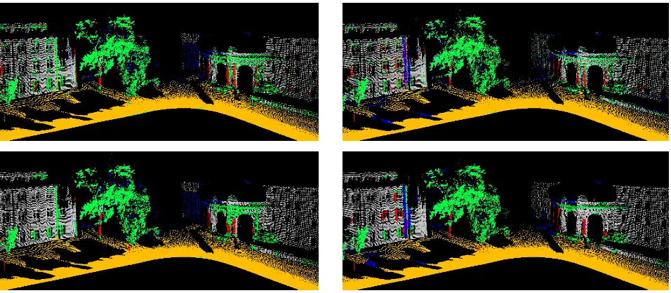
Figure 1. Classified 3D point clouds for the neighborhoods{N50,Nopt,λ}(left and right column) and the classifiersRF200,CRF 5 200
(top and bottom row) when using a standard color encoding (wire: blue;pole/trunk: red;fac¸ade: gray;ground: brown;vegetation: green). Note the noisy appearance of the results for individual point classification (top row).
the differences in quality for the classesw,p/tandfshow higher variations. It becomes obvious that if the better base classifier (RF200) is used, these classes are differentiated best by using an
adaptive neighborhood as in variantNopt,λ, in case of classp/tby
a large margin. The weight of the interaction potential does have an impact on the results, but at least in those cases where200 trees are used for the association potentials, the effect of chang-ing the weight in the range tested here is relatively low compared to the impact of using the interactions in the first place. The value w1= 5.0seems to be a good trade-off in this application.
One can see from our results that the main impact of using inter-actions in classification consists of a considerable improvement in the classification performance of classes that are not dominant in the data, which is consistent with the findings in (Niemeyer et al., 2014) for airborne laser scanning data. In the case of mo-bile laser scanning data, it might in fact be those classes one is mainly interested in. The most dominant classgcan easily be distinguished from the remaining data by simply considering height, and the respective completeness and correctness numbers do not vary much. In contrast,p/tmight for instance be a class of major interest for mapping urban infrastructure. When using a fixed neighborhoodN50and a Random Forest without
interac-tions (variant RF200), the completeness and the correctness of the
results are52.5% and42.0%, respectively, resulting in a quality of30.4% (Table 3). Nearly half of the points on poles or trunks are not correctly detected, and more than half of the points clas-sified asp/tare in fact not situated on poles or trunks. Using the neighborhoodNopt,λand a CRF (CRF
5
200), these numbers are
in-creased to a completeness of78.8% and a correctness of59.7% (cf. Table 7), which results in a quality of51.4% and certainly provides a better starting point for subsequent processes.
5 CONCLUSIONS
In this paper, we have presented a generic approach for automated 3D scene analysis. The novelty of this approach addresses the interrelated issues of (i) neighborhood selection, (ii) feature ex-traction and (iii) contextual classification, and it consists of using individual 3D neighborhoods of optimal size for the subsequent steps of feature extraction and contextual classification. The re-sults derived on a standard benchmark dataset clearly indicate the
beneficial impact of involving contextual information in the clas-sification process and that using individual 3D neighborhoods of optimal size significantly increases the quality of the results for both pointwise and contextual classification.
For future work, we want to carry out deeper investigations con-cerning the influence of the amount of training data as well as the influence of the number of different classes on the classifica-tion results for different datasets. Moreover, we intend to exploit the results of contextual point cloud classification for extracting single objects in a 3D scene such as trees, cars or traffic signs.
REFERENCES
Belton, D. and Lichti, D. D., 2006. Classification and segmentation of ter-restrial laser scanner point clouds using local variance information. The International Archives of the Photogrammetry, Remote Sensing and Spa-tial Information Sciences, Vol. XXXVI-5, pp. 44–49.
Blomley, R., Weinmann, M., Leitloff, J. and Jutzi, B., 2014. Shape dis-tribution features for point cloud analysis – A geometric histogram ap-proach on multiple scales.ISPRS Annals of the Photogrammetry, Remote Sensing and Spatial Information Sciences, Vol. II-3, pp. 9–16.
Boykov, Y. Y. and Jolly, M.-P., 2001. Interactive graph cuts for optimal boundary and region segmentation of objects in N-D images. Proceed-ings of the IEEE International Conference on Computer Vision, Vol. 1, pp. 105–112.
Breiman, L., 2001. Random forests.Machine Learning, 45(1), pp. 5–32. Bremer, M., Wichmann, V. and Rutzinger, M., 2013. Eigenvalue and graph-based object extraction from mobile laser scanning point clouds.
ISPRS Annals of the Photogrammetry, Remote Sensing and Spatial Infor-mation Sciences, Vol. II-5/W2, pp. 55–60.
Brodu, N. and Lague, D., 2012. 3D terrestrial lidar data classification of complex natural scenes using a multi-scale dimensionality criterion: applications in geomorphology. ISPRS Journal of Photogrammetry and Remote Sensing, 68, pp. 121–134.
Carlberg, M., Gao, P., Chen, G. and Zakhor, A., 2009. Classifying urban landscape in aerial lidar using 3D shape analysis. Proceedings of the IEEE International Conference on Image Processing, pp. 1701–1704. Chehata, N., Guo, L. and Mallet, C., 2009. Airborne lidar feature se-lection for urban classification using random forests. The International Archives of the Photogrammetry, Remote Sensing and Spatial Informa-tion Sciences, Vol. XXXVIII-3/W8, pp. 207–212.
Demantk´e, J., Mallet, C., David, N. and Vallet, B., 2011. Dimension-ality based scale selection in 3D lidar point clouds. The International Archives of the Photogrammetry, Remote Sensing and Spatial Informa-tion Sciences, Vol. XXXVIII-5/W12, pp. 97–102.
Filin, S. and Pfeifer, N., 2005. Neighborhood systems for airborne laser data. Photogrammetric Engineering & Remote Sensing, 71(6), pp. 743– 755.
Frey, B. J. and MacKay, D. J. C., 1998. A revolution: belief propagation in graphs with cycles.Proceedings of the Neural Information Processing Systems Conference, pp. 479–485.
Guan, H., Li, J., Yu, Y., Wang, C., Chapman, M. and Yang, B., 2014. Us-ing mobile laser scannUs-ing data for automated extraction of road markUs-ings.
ISPRS Journal of Photogrammetry and Remote Sensing, 87, pp. 93–107. Guo, B., Huang, X., Zhang, F. and Sohn, G., 2014. Classification of airborne laser scanning data using JointBoost. ISPRS Journal of Pho-togrammetry and Remote Sensing, 92, pp. 124–136.
Guyon, I. and Elisseeff, A., 2003. An introduction to variable and feature selection.Journal of Machine Learning Research, 3, pp. 1157–1182. Heipke, C., Mayer, H., Wiedemann, C. and Jamet, O., 1997. Evaluation of automatic road extraction.The International Archives of the Photogram-metry, Remote Sensing and Spatial Information Sciences, Vol. XXXII/3-4W2, pp. 151–160.
Hu, H., Munoz, D., Bagnell, J. A. and Hebert, M., 2013. Efficient 3-D scene analysis from streaming data. Proceedings of the IEEE Interna-tional Conference on Robotics and Automation, pp. 2297–2304. Jutzi, B. and Gross, H., 2009. Nearest neighbour classification on laser point clouds to gain object structures from buildings. The International Archives of the Photogrammetry, Remote Sensing and Spatial Information Sciences, Vol. XXXVIII-1-4-7/W5.
Khoshelham, K. and Oude Elberink, S. J., 2012. Role of dimensionality reduction in segment-based classification of damaged building roofs in airborne laser scanning data.Proceedings of the International Conference on Geographic Object Based Image Analysis, pp. 372–377.
Kumar, S. and Hebert, M., 2006. Discriminative random fields. Interna-tional Journal of Computer Vision, 68(2), pp. 179–201.
Lafarge, F. and Mallet, C., 2012. Creating large-scale city models from 3D-point clouds: a robust approach with hybrid representation. Interna-tional Journal of Computer Vision, 99(1), pp. 69–85.
Lafferty, J. D., McCallum, A. and Pereira, F. C. N., 2001. Conditional random fields: probabilistic models for segmenting and labeling sequence data.Proceedings of the International Conference on Machine Learning, pp. 282–289.
Lalonde, J.-F., Unnikrishnan, R., Vandapel, N. and Hebert, M., 2005. Scale selection for classification of point-sampled 3D surfaces. Proceed-ings of the International Conference on 3-D Digital Imaging and Model-ing, pp. 285–292.
Lee, I. and Schenk, T., 2002. Perceptual organization of 3D surface points.The International Archives of the Photogrammetry, Remote Sens-ing and Spatial Information Sciences, Vol. XXXIV-3A, pp. 193–198. Lim, E. H. and Suter, D., 2009. 3D terrestrial lidar classifications with super-voxels and multi-scale conditional random fields.Computer-Aided Design, 41(10), pp. 701–710.
Linsen, L. and Prautzsch, H., 2001. Local versus global triangulations.
Proceedings of Eurographics, pp. 257–263.
Lodha, S. K., Fitzpatrick, D. M. and Helmbold, D. P., 2007. Aerial li-dar data classification using AdaBoost. Proceedings of the International Conference on 3-D Digital Imaging and Modeling, pp. 435–442. Lu, Y. and Rasmussen, C., 2012. Simplified Markov random fields for ef-ficient semantic labeling of 3D point clouds.Proceedings of the IEEE/RSJ International Conference on Intelligent Robots and Systems, pp. 2690– 2697.
Mallet, C., Bretar, F., Roux, M., Soergel, U. and Heipke, C., 2011. Rele-vance assessment of full-waveform lidar data for urban area classification.
ISPRS Journal of Photogrammetry and Remote Sensing, 66(6), pp. S71– S84.
Mitra, N. J. and Nguyen, A., 2003. Estimating surface normals in noisy point cloud data. Proceedings of the Annual Symposium on Computa-tional Geometry, pp. 322–328.
Munoz, D., Bagnell, J. A., Vandapel, N. and Hebert, M., 2009. Contextual classification with functional max-margin Markov networks.Proceedings of the IEEE Conference on Computer Vision and Pattern Recognition, pp. 975–982.
Niemeyer, J., Rottensteiner, F. and Soergel, U., 2014. Contextual classi-fication of lidar data and building object detection in urban areas.ISPRS Journal of Photogrammetry and Remote Sensing, 87, pp. 152–165.
Niemeyer, J., Wegner, J. D., Mallet, C., Rottensteiner, F. and Soergel, U., 2011. Conditional random fields for urban scene classification with full waveform lidar data.Photogrammetric Image Analysis, LNCS 6952, Springer, Heidelberg, Germany, pp. 233–244.
Osada, R., Funkhouser, T., Chazelle, B. and Dobkin, D., 2002. Shape distributions.ACM Transactions on Graphics, 21(4), pp. 807–832. Pauly, M., Keiser, R. and Gross, M., 2003. Multi-scale feature extraction on point-sampled surfaces.Computer Graphics Forum, 22(3), pp. 81–89. Pu, S., Rutzinger, M., Vosselman, G. and Oude Elberink, S., 2011. Recog-nizing basic structures from mobile laser scanning data for road inventory studies. ISPRS Journal of Photogrammetry and Remote Sensing, 66(6), pp. S28–S39.
Rusu, R. B., Marton, Z. C., Blodow, N. and Beetz, M., 2008. Persistent point feature histograms for 3D point clouds.Proceedings of the Interna-tional Conference on Intelligent Autonomous Systems, pp. 119–128. Schmidt, A., Niemeyer, J., Rottensteiner, F. and Soergel, U., 2014. Con-textual classification of full waveform lidar data in the Wadden Sea.IEEE Geoscience and Remote Sensing Letters, 11(9), pp. 1614–1618. Schmidt, A., Rottensteiner, F. and Soergel, U., 2012. Classification of airborne laser scanning data in Wadden Sea areas using conditional ran-dom fields. The International Archives of the Photogrammetry, Remote Sensing and Spatial Information Sciences, Vol. XXXIX-B3, pp. 161–166. Schmidt, A., Rottensteiner, F. and Soergel, U., 2013. Monitoring con-cepts for coastal areas using lidar data.The International Archives of the Photogrammetry, Remote Sensing and Spatial Information Sciences, Vol. XL-1/W1, pp. 311–316.
Secord, J. and Zakhor, A., 2007. Tree detection in urban regions using aerial lidar and image data. IEEE Geoscience and Remote Sensing Let-ters, 4(2), pp. 196–200.
Serna, A. and Marcotegui, B., 2013. Urban accessibility diagnosis from mobile laser scanning data. ISPRS Journal of Photogrammetry and Re-mote Sensing, 84, pp. 23–32.
Serna, A. and Marcotegui, B., 2014. Detection, segmentation and classi-fication of 3D urban objects using mathematical morphology and super-vised learning. ISPRS Journal of Photogrammetry and Remote Sensing, 93, pp. 243–255.
Shannon, C. E., 1948. A mathematical theory of communication. The Bell System Technical Journal, 27(3), pp. 379–423.
Shapovalov, R., Velizhev, A. and Barinova, O., 2010. Non-associative Markov networks for 3D point cloud classification. The International Archives of the Photogrammetry, Remote Sensing and Spatial Information Sciences, Vol. XXXVIII-3A, pp. 103–108.
Shapovalov, R., Vetrov, D. and Kohli, P., 2013. Spatial inference ma-chines. Proceedings of the IEEE Conference on Computer Vision and Pattern Recognition, pp. 2985–2992.
Shotton, J., Winn, J., Rother, C. and Criminisi, A., 2009. TextonBoost for image understanding: multi-class object recognition and segmentation by jointly modeling texture, layout, and context. International Journal of Computer Vision, 81(1), pp. 2–23.
Velizhev, A., Shapovalov, R. and Schindler, K., 2012. Implicit shape models for object detection in 3D point clouds. ISPRS Annals of the Photogrammetry, Remote Sensing and Spatial Information Sciences, Vol. I-3, pp. 179–184.
Wegner, J. D., Soergel, U. and Rosenhahn, B., 2011. Segment-based building detection with conditional random fields. Proceedings of the Joint Urban Remote Sensing Event, pp. 205–208.
Weinmann, M., Jutzi, B. and Mallet, C., 2013. Feature relevance as-sessment for the semantic interpretation of 3D point cloud data. ISPRS Annals of the Photogrammetry, Remote Sensing and Spatial Information Sciences, Vol. II-5/W2, pp. 313–318.
Weinmann, M., Jutzi, B. and Mallet, C., 2014. Semantic 3D scene inter-pretation: a framework combining optimal neighborhood size selection with relevant features. ISPRS Annals of the Photogrammetry, Remote Sensing and Spatial Information Sciences, Vol. II-3, pp. 181–188. West, K. F., Webb, B. N., Lersch, J. R., Pothier, S., Triscari, J. M. and Iverson, A. E., 2004. Context-driven automated target detection in 3-D data.Proceedings of SPIE, Vol. 5426, pp. 133–143.
Xiong, X., Munoz, D., Bagnell, J. A. and Hebert, M., 2011. 3-D scene analysis via sequenced predictions over points and regions. Proceed-ings of the IEEE International Conference on Robotics and Automation, pp. 2609–2616.
Xu, S., Vosselman, G. and Oude Elberink, S., 2014. Multiple-entity based classification of airborne laser scanning data in urban areas.ISPRS Jour-nal of Photogrammetry and Remote Sensing, 88, pp. 1–15.
![Table 2. Quality q [%] for class w achieved in all experiments.](https://thumb-ap.123doks.com/thumbv2/123dok/3205107.1393383/6.595.300.540.75.639/table-quality-q-class-w-achieved-experiments.webp)