RANDOM FORESTS BASED MULTIPLE CLASSIFIER SYSTEM FOR POWER-LINE
SCENE CLASSIFICATION
H. B. Kim-a, G. Sohn-a a-
GeoICT Lab, Earth and Space Science and Engineering Department, York University, 4700 Keele St., Toronto, ON M3J 1P3, Canada – (hskim, gsohn)@yorku.ca
Commission III, WG III/4
KEY WORDS: LIDAR, Classification, Corridor Mapping, Random Forests, Multiple Classifier System, Power-line
ABSTRACT:
The increasing use of electrical energy has yielded more necessities of electric utilities including transmission lines and electric pylons which require a real-time risk monitoring to prevent massive economical damages. Recently, Airborne Laser Scanning (ALS) has become one of primary data acquisition tool for corridor mapping due to its ability of direct 3D measurements. In particular, for power-line risk management, a rapid and accurate classification of power-line objects is an extremely important task. We propose a 3D classification method combining results obtained from multiple classifier trained with different features. As a base classifier, we employ Random Forests (RF) which is a composite descriptors consisting of a number of decision trees populated through learning with bootstrapping samples. Two different sets of features are investigated that are extracted in a point domain and a feature (i.e., line & polygon) domain. RANSAC and Minimum Description Length (MDL) are applied to create lines and a polygon in each volumetric pixel (voxel) for the line & polygon features. Two RFs are trained from the two groups of features uncorrelated by Principle Component Analysis (PCA), which results are combined for final classification. The experiment with two real datasets demonstrates that the proposed classification method shows 10% improvements in classification accuracy compared to a single classifier.
1. INTRODUCTION
Airborne Laser Scanning (ALS) data is a promising data source being able to cost-effectively cover a huge area and possessing an advantage of direct 3D measurement with high density, high accuracy, and multiple echoes compared to other remote sensed data. ALS has been mainly utilized for Digital Terrain Model (DTM) data, urban management, costal line detection, etc. Recently, many power-line industries are using ALS for the purpose of the risk management of electric utilities such as transmission lines and electric pylons. Currently, 340,000 km of power networks have been installed across entire North America continent (NERC). The complicatedly connected power-line network requires a regular monitoring to ensure a reliable supply of electric power. Otherwise, a considerable amount of economical loss and inconvenience might happen as Northeast Blackout of 2003. To prevent such a disaster in advance, most of utility firms are trying to build their own risk management system to deliver vegetation clearance report and mitigate possible risks within few days. However, current status of the state-of-the art technologies still involves labour-centric processing, in particular for scene classification. Thus, an automated classification method is urgently required to realize the rapid corridor mapping.
In this study, we extend our previous research by investigating object-based features (i.e. features that are structured in line and polygon). In fact, key objects comprising power-line scene such as wire and pylon can be viewed as lines and their associations, while building as polygon objects, and vegetation as non-structured object. Compared to point-based feature, the object-based feature provides certain advantageous aspects for classification purpose. For instance, the object-based feature is useful to analyze a group of points if they are a structured object or non-structured one. In addition, it also provides an
opportunity to analyze contextual properties between features (e.g., a relation of line-line, line-polygon, polygon-polygon). In this research, we aims to investigate complementary role of object-based feature compared to point-based one and develop a Multiple Classifier System (MCS) to synergistically fuse the classification results obtained from each feature for power-line scene classification.
2. PREVIOUS RESEARCH
Many researches on classification are carried out in various ways according to data source and target object. Baillard & Maître (1999) represented elevation data as a node and an edge potential function based on Markov Random Field (MRF) in order to identify ground. For extracting bare-earth surface, Lu et al. (2009) introduced three types of features (i.e., point-features, segment-feature, and disc-feature) from ALS incorporated in Conditional Random Field (CRF). Not many researches related to power utilities including classification and modelling have been reported. Kim & Sohn (2010) proposed a point- and voxel-scaled feature extraction and 3D classification using Random Forests in power-line scene where a few structures such as wire, building, pylon, and vegetation would be vertically overlapped. Jwa et al. (2009) introduced an automatic algorithm to reconstruct 3D transmission models from ALS point of clouds using non-linear least square regression method. McLaughlin (2006) performed transmission line identification by applying Gaussian mixture model to eigenvalues computed from ellipsoid neighbourhoods and transmission line modelling by iteratively estimating model parameters using the tangent to the span at each point. Melzer & Briese (2004) extracted power lines from LIDAR data using iterative Hough transform (HT) and modelled them by grouping close reference vectors quantized by Neural Gas Network.
Feature design and feature extraction are important steps in pattern recognition and classification. Lipson & Shpitalni (1996) defined 13 regularities between lines for 3D object reconstruction from a single freehand line drawing. Certain regularities or features may correspond to noise and thus do not have any information due to correlation between them. Therefore, regularity or feature selection is necessary for effective 3D object reconstruction from a single line drawing (Yuan et al., 2008). Elder & Goldberg (2002) suggested a perceptual contour grouping from natural images by applying the inferential power of three classical Gestalt cues: proximity, good continuation, and luminance similarity. They represented the quantitative description of three cues as likelihood distribution by training samples in order to calculate posterior probability distribution under Bayesian framework. Rutzinger et al. (2008) used surface roughness, point density ratio of 2D to 3D domain, and echo information as well as FW features for urban vegetation classification. In this research, RANSAC and Minimum Description Length (MDL) were employed to produce line and polygon objects for additional feature extraction (Yang & Förstner, 2010).
Another classification approach is to adopt the machine learning technique, which can yield a decision boundary or a decision classifier. Lodha et al. (2006, 2007) applied SVM and AdaBoost to ALS data using class- and sample-weighted feature values. Random Forests is one of the state-of-the-art classification methods (Chehata et al., 2009). Narayanan et al. (2009) applied ensemble classifiers to generate under-water habitat maps using FW data collected by SHOALS 3000. The Multiple Classifier System (MCS) makes a final decision by combining a set of classifiers. Suutala & Roning (2005) presented a MCS consisting of two combination stages: classifier fusion from features and classifier fusion from samples in order for person identification from footstep. Samadzadegan et al. (2010) proposed a classifier fusion composed of one-against-one SVM and one-against-all SVM learned from a feature set for ALS data classification.
3. ENSEMBLE CLASSIFIER & MCS 3.1 Ensemble classifier
RF is a combination of a number of decision trees which are generated by learning instance groups sampled independently from a training set (Breiman, 2001). Each tree is branched off by splitting the nodes on a limited number of features randomly selected from input vector until they are impure in terms of class. Such random feature selection promotes the diversity of trees, and it improves classification performance at the end. After an ensemble of trees is populated, the final prediction is a majority vote of their individual predictions. We defined
confidence value of each class as a proportion of votes of
corresponding class. Several setup variables are necessary to run RF: the number of input features (M), the number of features randomly selected (F) and the number of populated trees (T). The larger M is, the more complicated each tree is. That is, RF might lead to overestimated decision trees. To avoid this problem, important feature selection is required. F is estimated as the first integer less than log2M+1 (Breiman, 2001). In addition to RF, the well-known ensemble methods are bagging where lots of sets of instances called bootstrap replicates randomly drawn from a training data grow an ensemble of trees (Breiman, 1996) and boosting which increases its performance by more considering the misclassified instances in the previous decision (McIver et al, 2002). However, bagging is likely to make similar decision trees due to
the likeness to the bootstrapping samples and boosting tends to lead to poor performance on data with noise because it would regard noises as misclassified cases (Dietterich, 2000).
3.2 Multiple classifier system
Information fusion stands for the data fusion from different sources: sensory data, patterns, features, decisions, knowledge, classifier and so on. Multiple Classifier System means classifier fusion among the information fusion. MCS is a combination of a group of classifiers and its advantage is to reduce the risk of choosing a poor classifier in Single Classifier System (SCS) by considering all classifiers for a decision (Dara, 2007). Generally, there are two types of structures for MCS construction: parallel
and cascade. The parallel MCS is more common architecture.
All classifiers comprising of the MCS operate in parallel and their predictions are combined for a final decision. The combination strategies are maximum, minimum, sum, product,
median, majority vote, averaging as simple ways and fuzzy
integrals, weighted averaging, decision templates, and logistic
regression as complicated ways (Dara, 2007). On the contrary,
classifiers of the sequential MCS are applied in sequence, that is, an output of a classifier is used as an input of next classifier. This decreases a problem complexity, but the performance of each classifier extremely depends on that of its previous classifier. We choose the parallel MCS because two sets of input features are independent and sum rule due to the use of exactly same classifier (Sum rule works well with similar classifier). Sum rule makes a final decision by choosing a class corresponding to the highest value after adding confidence values from each classifier.
4. METHOD
In this research, our goal is to classify unlabeled power-line corridors into vegetation, wire, pylon, and building. Terrain is not an interesting class in this paper. Therefore, we are supposing that terrain has been identified by an independent terrain filtering algorithm.
4.1 Feature extraction 4.1.1 Point-based features
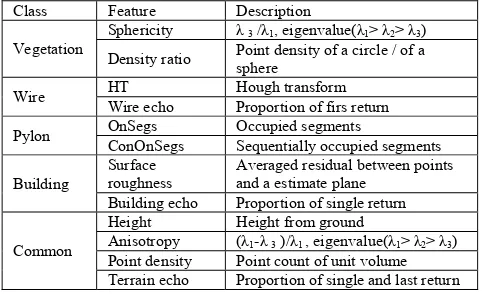
Kim & Sohn (2010) investigated 21 features which enable to classify vegetation, wire, pylon, and building. For each point, they were computed with neighbouring points taken in a sphere with fixed radius. They then selected 12 out of 21 features according to the importance estimated by Random Forests: two important features for each class and four common features as shown in Table 1.
Table 1. 12 important features in power-line scene (Kim & Sohn, 2010).
Class Feature Description
Vegetation
Sphericity λ3 /λ1, eigenvalue(λ1> λ2> λ3)
Density ratio Point density of a circle / of a sphere
Wire HT Hough transform
Wire echo Proportion of firs return
Pylon OnSegs Occupied segments
ConOnSegs Sequentially occupied segments
Building
Surface roughness
Averaged residual between points and a estimate plane
Building echo Proportion of single return
Common
Height Height from ground
Anisotropy (λ1-λ3 )/λ1 , eigenvalue(λ1> λ2> λ3)
Point density Point count of unit volume Terrain echo Proportion of single and last return
There would exist correlations and dependencies between the features above. Therefore, we applied Principle Component Analysis (PCA) to remove such factors. The amount of information loss was limited less than 5%. As a result of PCA, 6 largest principle components were selected, that is, the dimension of feature space was reduced from 12 to 6.
4.1.2 Object-based features
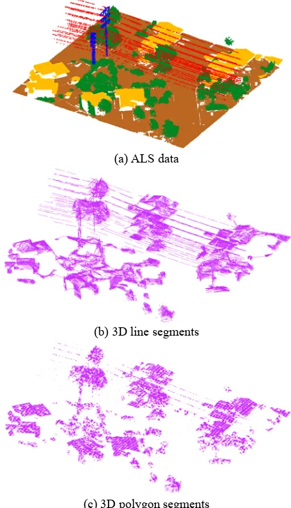
A feature presented by a set of points belonging to a group can be augmented if they are truly a part of an object. From this viewpoint, wire and pylon can be typically decomposed into line, but pylon is close to line as low voltage type. On the other hand, building can be depicted as plane. Vegetation tends to be neither line nor plane (i.e., non-structured object). After voxel segmentation of 3D points, RANSAC and Minimum Description Length (MDL) were applied to produce line and plane segments for each occupied voxel (Ying & Förstner, 2010). Unlike features from point domain, features from object domain have contexture properties between objects. For instance, colinearity indicates averaged angle difference between neighbours topologically placed at previous and next from a certain line. A 3D polygon and multiple 3D lines are generated in each voxel (Figure 1). This is because there might exist two more wires in the volume. The voxel sizes for line and polygon generation are 1.5m and 15m respectively.
The follows are the features extracted from line models. Line segments within a buffer volume produced from a certain line are chosen as neighbours of the line.
Line slope: is the angle from XY plane to the line. Pylon is mostly vertical structure, so its line slope tends to be 90 degrees.
Line residual: is the averaged orthogonal distance from points to the line segment. Wire is small, but vegetation and building is large on this.
In-out shell: Two different radius cylinders (in-out shell) are produced from the line segment. This feature stands for the ratio of number of points existing within inner and outer shell. Wire does not have any points in outer shell generally.
Orientation direction difference: is to highlight wire which typically has same orientation direction. This feature indicates the orientation angle difference between a line and its neighbours projected on XY plane.
Parallelism: means the magnitude of that a line is parallel to its side lines. Most wires are parallel each other.
Structurality: Components of most man-made structures tend to be structurally regular, e.g., angles between struts of a truss bridge are likely to be 0, 45, and 90 degrees for an effective support. Similarly, struts of an electric pylon commonly form the regular angles. Thus, if angle difference between a target line and its neighbours is close to 0, 45, and 90 degrees, a high value is assigned to the line. Wire can is highlighted as well.
Colinearity: is the averaged angle difference between lines. Wires and some of pylons could be characterized.
Orthogonality: is opposite to colinearity. Parts of pylon would have high values, but wire is small.
Standard deviation of line slope: is a root mean squared slope difference of lines along a voxel column. Lines corresponding to vegetation would be randomly populated, so vegetation is
high. Building lines are also randomly generated, but their line slopes are mostly same because they lie on a plane. Wire and pylon lines have similar slope.
(a) ALS data
(b) 3D line segments
(c) 3D polygon segments
Figure 1. Line and polygon segments creation from LIDAR.
Number of crossing lines: A set of points within each voxel were used to generate multiple lines until the derivative of total line description score changes from negative to positive or the number of created lines reaches a given threshold. As the result, most vegetation and most building produced maximum number of line models. This presents the number of generated models in a voxel.
Line description length: is the ration of total description lengths when supposed there is no model and when lines are created. Wire and pylon are expected to be high.
The next lists the features extracted from polygon models. Each occupied voxels generates a 3D polygon. 26 adjacent voxels to a voxel including a target polygon are considered as neighbours. Polygon slope: is slope of plane with respect to XY plane. Polygon from pylon is expected to be vertical.
Polygon residual: Averaged orthogonal distance to a polygon. This feature is small in building.
Ground frequency: is the proportion of ground under a polygon. There is rarely ground under building polygon.
Surface normal difference: is an averaged surface normal difference of a polygon and adjacent polygons. Building with gentle roof slope might be approximately zero degree.
Perpendicularity: is a contrary feature to surface normal
difference. If surface normal difference equals to 90 degrees
(i.e., adjacent polygons are perpendicular), this feature is maximum.
Standard deviation of surface normal: This feature is a root mean squared surface normal difference of a set of polygons close to each other. This is a feature for building.
Polygon description length: is the ration of total description lengths when supposed no model and when polygons are created. Building would be high.
All points are not used to model lines or polygons, so features of the unused points are brought from the nearest line or polygon. After that, all feature values are normalized using bipolar sigmoidal distribution [-1, +1] and the features then are projected by PCA to remove correlations between them. For object feature, PCA chose 11 largest principle components out of 18.
4.1.3 Validation of Object-based feature
For generating object-based feature, we conduct a “blind” segmentation approach, in which all points captured in a voxel are forced to be converted into either line or polygon regardless of the true classes. This “blind” segmentation might cause some problems. For instance, parallel lines are produced from building points whose space is fairly regular, and coplanar polygons were occasionally yielded from wire (especially, bundled conductors) and pylon. Therefore, an additional step is necessary to validate whether the generated lines and the generated polygons are populated from real line objects and real polygon objects or not.
(a) Before line validation (b) After line validation Figure 2. Effectiveness of line feature validation on
Structurality (x-axis is normalized feature values [-1,+1]).
For line validation, we first picked up points existing within a buffer from each line segment, and then rotated them through the angle between the line and XY plane in order to project them on XY plane. After that, their xy were converted into Hough domain. The ratio of global maximum in the Hough accumulator to the number of taken points was multiplied by line features to augment them. Secondly, we validate polygons through computing the ratio of points composing of each polygon to its outline points, and then we multiplied the ratio by polygon features. Polygon from building would be larger than polygons from the other classes in terms of the ratio value because building polygon possesses relatively more points inside. Figure 2 shows an effectiveness of line validation which produces distinguishable distributions of vegetation and pylon.
4.2 Prediction fusion
Random Forests (RF) enables to output the confidence value of each class. From point-based features and object-based features extracted in section 4.1.1 and 4.1.2, we generate two different
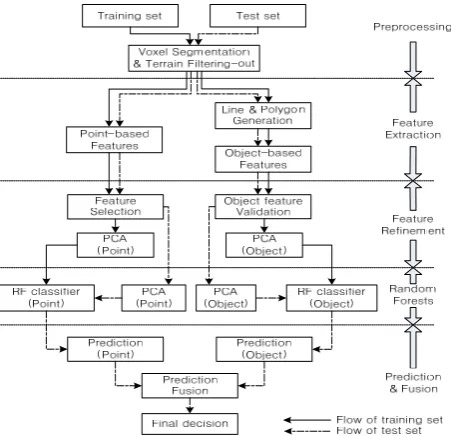
RF classifiers on a same dataset. As mentioned in section 3.2, we determined a parallel MCS of prediction fusion because two feature extraction methods are independent. For a combination strategy, we employed “Sum Rule” because both classifiers are populated in a same way, Random Forests (Dara, 2007). That is, confidence values voted by two classifiers are added for each class. Finally, a class with maximum confidence is chosen as a final prediction. Figure 3 delineates an entire workflow from feature extraction to classifier combination.
Figure 3. Flow chart of Random Forest based MCS classification for training and testing.
The expected effectiveness of MCS is a decrease of classification error by complementing each classifier. RF classifier from point feature more focuses on classification and RF classifier from line & polygon features once more validates predictions of the other classifier which are not confident.
5. EXPERIMENTAL RESULT 5.1 Experiment data
We tested three subsets taken from two different corridors of high voltage type in California, USA. They were collected by LMS-Q560 of Riegl with 30/m2 of the point density on average. Two subsets from a scene were picked up for training and testing. One more subset was taken from a different scene from the previous one to evaluate a reliability of our approach. The two test sets are denoted TE#1 and TE#2 respectively, and training set is denoted TR. All datasets include vegetation, wire, electric pylon, and building. Additional major class contained in the test scenes is fence object, but we do not take into account of this object for classification for current study. TR and TE#1 contain 115kV and 230kV transmission lines, lattice type of pylons, gable roofed type of buildings, and leaf-on trees. Moreover, most parts of 230kV conductors consist of two bundled wires. There are 230kV single conductor, steel pole type of pylon, gable building, and leaf-on trees in TE#2. Both of them are categorized into high voltage type according to American National Standards Institute (ANSI).
5.2 Point-based RF (PRF) and Object-based RF (ORF) Kim & Sohn (2010) introduced a classification method using Random Forests from point features. Here PRF is same as their
method, but we applied features uncorrelated by PCA using 12 chosen critical features to Random Forests. Consequently, 6 principle components were retained. For RF the number of random features is set F=3 following the equation described in section 3.1, in our case M=6. The ORF takes 11 principle components from 18-dimensional feature space, so F=4.
Table 2. Confusion matrix for TE#1 using PRF (F=3, T=60)
Class Veget Wire Pylon Bldg Recall (%)
Veget 48,120 40 30 1224 97.38
Wire 114 8,416 242 113 94.72
Pylon 7 93 1,298 9 92.25
Bldg 1,490 13 0 92,206 97.95
Precision (%) 97.02 99.39 90.88 99.15
Table 3. Confusion matrix for TE#1 using ORF (F=4, T=60)
Class Veget Wire Pylon Bldg Recall (%)
Veget 46,564 379 1,575 896 94.23
Wire 128 8,412 55 20 97.64
Pylon 321 44 1,031 11 73.28
Bldg 5,049 191 132 88,337 94.27
Precision (%) 89.44 93.20 36.91 98.96
The numbers in Table 2 and 3 stand for point count. The confusion matrices present that PRF seems to be better than ORF. However, they are not competitors each other, but complementers for next fusion step. A lattice steel pylon which is a steel framework construction caused an accuracy decrease of pylon in ORF because some of line features for the pylon were not extracted incorrectly. Each of PRF and ORF recorded 97.5% and 94.3% overall performance.
Figure 4. Classification error for TE#1
5.3 Combination of two predictions
The second experiment is to combine two predictions that are confidence values for each class, resulted by PRF and ORF. As shown in figure 4, the omission errors and commission errors were simultaneously declined thanks to complementary activity between two success rates to 98.5% and the accuracy for all classes was also much better than that of each single classifier. Thus, the advantage of our MCS is that ORF validates errors from PRF once more. However, we cannot guarantee our MCS is superior to PRF or ORF in all cases (Dara, 2007).
Figure 5 depicts how PRF and ORF are complementary. In PRF, 10 % of misclassification cases are strongly confident even if they are false confidences. Such false confidences were disappeared by combining classifiers. Probably, false confidences with some of misclassification cases might change into true confidences or their values would decrease.
Figure 5. Difference between confidences corresponding to predicted class and true class in case of misclassification inTE#1.
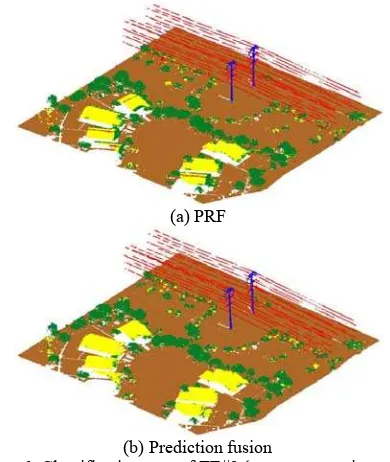
5.4 Classification on different scene (same voltage type) To validate our approach, we applied it to another data set (TE#2) taken from different source (from different site and at different time). As TE#2 has different scene characteristics from TR, point-based features respectively extracted from two data might be different. However, object-based features would be invariant (wire is always linear, building planar, pylon vertical, and vegetation scattering). PRF seems to be very sensitive to data source. There exist numbers of clear omission errors of building incorrectly committed into wire and vegetation. Some of wire points were classified into pylon (Figure 6-a). This does not happen in real. Lots of such obvious errors were corrected by our suggested method (Figure 6-b). However, confusion between vegetation and building still exist when they are close or when vegetation are not broadly thick with leaves such as low vegetation. Quantitatively, the class overall success rate increased from 83.0% to 93.9%.
(a) PRF
(b) Prediction fusion
Figure 6. Classification map of TE#2 (green: vegetation, red: wire, blue: pylon, and yellow: building)
6. CONCLUSIONS
We suggested random forests based multiple classifier system for power-line scene classification from airborne laser scanning data. For the RF, we investigated two sets of features respectively extracted from two different domains: 12 features from point domain and 18 features from line & polygon domain. PCA was then applied to the features in order to eliminate correlations and dependencies between them. At the end, 6 and
11 principle components were retained among point features and line & polygon features respectively. It seems that PRF generally performs well on the data sets from same sources as learning set and better than ORF, but there are still a number of errors which are regarded as obvious misclassification. Therefore, we designed another classifier which is able to remove such clear errors as possible by complementing each other. ORF was invented for the purpose of validation of PRF. That is, line- & polygon-based classifier encourages point-based classifier to judge better by adding confidence when the decision is not obvious. We observed not only the decrease in both omission and commission error but also the increase in performance after combining the results of two classifiers. We tested a new data (TE#2) taken from a different site to validate our approach. As a result of the experiment, 93.9% classification performance was achieved. RF-based MCS resulted in 10% improvement compared to PRF. Therefore, we conclude the suggested approach is not definitely sensitive to data source.
ACKNOWLEDGEMENTS
We would like to acknowledge the financial support of Ontario Centres of Excellence (OCE) and Geo Digital International (GDI) for the project named “Spatiotemporal Risk Management of Power-line Networks”. We thank again GDI which has provided Airborne Laser Scanning data for experiments in this study. We used Weka 3.5 for Random Forests customized by Livingston, F. It is appreciated that he published it.
REFERENCES
Baillard, C. and Maître, H., 1999, 3D Reconstruction of Urban Scenes from Aerial Stereo Imagery: A Focusing Strategy, Computer Vision and Image Understanding, vol. 76, no. 3, pp. 244–258.
Breiman, L., 1996, Bagging Predictors, Machine Learning, Vol. 24, No. 2, pp. 123-140
Breiman, L., 2001, Random Forests, Machine Learning, Vol. 45, No. 1, pp. 5-32
Chehata, N., Guo, L., Mallet, C., 2009. Airborne lidar feature selection for urban classification using random forests. In: Laser scanning 2009, IAPRS, Vol. XXXVIII, Part 3/W8 – Paris, France, September 1-2, pp. 207-212.
Dara, R.A., 2007. Cooperative Training in Multiple Classifier Systems; thesis :Doctor of Philosophy; Waterloo, Ontario, Canada
Dietterich,T.G., 2000. Ensemble Methods in Machine Learning, First International Workshop on Multiple Classifier Systems. Springer Verlag, New York.
Elder, J. H. and Goldberg, R. M., 2002, Ecological statistics of Gestalt laws for the perceptual organization of contours, Journal of Vision, vol. 2, no. 4, pp. 324–353.
Jwa, Y., Sohn, G., Kim, H. B., 2009. Automatic detection and modeling of powerline from airborne laser scanning data. ISPRS Laserscanning 2009, September 1-4, Paris.
Kim, H. B. and Sohn, G., 2010. 3D Classification of Power-line Scene from Airborne Laser Scanning Data. Photogrammetric
Computer Vision (PCV) 2010, ISPRS Commission III Symposium, Vol. 38, September 1-3, Paris, France, pp. 207-212.
Lipson, H., and Shpitalni, M., 1996. Optimization-Based Reconstruction of a 3D Object from a Single Freehand Line Drawing,” Computer-Aided Design, vol. 28, no. 8, pp. 651-663.
Lodha, S. K., Fitzpatrick, D. M. and Helmbold, D. P., 2007. Aerial Lidar Data Classification using AdaBoost. In: International Conference on 3-D Digital Imaging and Modeling, Montreal, pp. 435–442.
Lodha, S. K., Kreps, E. J., Helmbold, D. P. and Fitzpatrick, D., 2006. Aerial LiDAR Data Classification Using Support Vector Machines (SVM). In: International Symposium on 3D Data Processing, Visualization and Transmission, IEEE, Chapel Hill, NC, pp. 567–574.
Lu, W. L., Murphy, K. P., Little, J. J., Sheffer, A., and Fu, H., 2009. A hybrid conditional random field for estimating the underlying ground surface from airborne Lidar data. IEEE-TGARS, 47(8/2): pp. 2913-2922.
McIver, D.K., Friedl, M.A., 2002, Using Prior Probabilities in Decision-Tree Classification of Remotely Sensed Data, Remote Sensing of Environment, Vol. 81, pp. 253-261.
McLaughlin, R. A., 2006. Extracting Transmission Lines From Airborne LIDAR Data, IEEE Geoscience and Remote Sensing Letters, Vol. 3, NO. 2, pp. 222-226.
Melzer, T., Briese, C., 2004. Extraction and modelling of power lines from ALS point clouds, in Proceedings of 28th Workshop of the Austrian Association for Pattern Recognition, pp.47-54.
Narayanan, R., Kim, H. B., Sohn, G., 2009. Classification of SHOALS 3000 Bathymetric LIDAR Signals Using Decision Tree and Ensemble Techniques, 2009 IEEE Toronto International Conference–Science and Technology for Humanity, pp. 26-27.
NERC, North American Electric Reliability Corporation. http://www.nerc.com (accessed 22 March. 2011)
Rutzinger, M., Höfle, B., Hollaus, M. & Pfeifer, N. 2008. Object-Based Point Cloud Analysis of Full-Waveform Airborne Laser Scanning Data for Urban Vegetation Classification. Sensors. Vol. 8(8), pp. 4505-4528.
Samadzadegan, F., Bigdeli, B., and Ramzi, R., 2010. A Multiple Classifier System for Classification of LIDAR Remote Sensing Data Using Multi-class SVM, Multiple Classifier Systems 9th International Workshop, MCS 2010, Cairo, Egypt, April 7-9, Proceedings.
Suutala, J., and Roning, J., 2005. Combining Classifier with Different Footstep Feature Sets and Multiple Samples for Person Identification, Proceeding of International Conference on Acoustics, Speech and Signal Processing, pp. 357-360.
Yang, M. Y. and Förstner, W., 2010. Plane Detection in Point Cloud Data Technical Report, Institute of Geodesy and Geoinformation, Department of Photogrammetry.
Yuan S., Tsui, L.Y. and Jie, S., 2008. Regularity selection for effective 3D object reconstruction from a single line drawing. Pattern Recognition Letters 29 (10), pp. 1486-1495.