VOLUME COMPUTATION OF A STOCKPILE
–
A STUDY CASE COMPARING GPS AND
UAV MEASUREMENTS IN AN OPEN PIT QUARRY
P. L. Raevaa, S. L. Filipovaa, D. G. Filipova
a University of Architecture, Civil Engineering and Geodesy, Faculty of Geodesy, Department of Photogrammetry and Cartography, Sofia, Bulgaria,
[email protected], [email protected], [email protected]
Commission ICWG I/Vb
KEY WORD: UAV photogrammetry, surveying of stockpiles, volumetric computation, GNSS technologies
ABSTRACT:
The following paper aims to test and evaluate the accuracy of UAV data for volumetric measurements to the conventional GNSS techniques. For this purpose, an appropriate open pit quarry has been chosen. Two sets of measurements were performed. Firstly, a stockpile was measured by GNSS technologies and later other terrestrial GNSS measurements for modelling the berms of the quarry were taken. Secondly, the area of the whole quarry including the stockpile site was mapped by a UAV flight. Having considered how dynamic our world is, new techniques and methods should be presented in numerous fields. For instance, the management of an open pit quarry requires gaining, processing and storing a large amount of information which is constantly changing with time. Fast and precise acquisition of measurements regarding the process taking place in a quarry is the key to an effective and stable maintenance. In other words, this means getting an objective evaluations of the processes, using up-to-date technologies and reliable accuracy of the results. Often legislations concerning mine engineering state that the volumetric calculations are to present ±3% accuracy of the whole amount. On one hand, extremely precise measurements could be performed by GNSS technologies, however, it could be really time consuming. On the other hand, UAV photogrammetry presents a fast, accurate method for mapping large areas and calculating stockpiles volumes. The study case was performed as a part of a master thesis.
1. INTRODUCTION
UAV photogrammetry has recently increased its popularity among numerous engineering spheres. Besides mapping and photogrammetric tasks, UAV perfectly complies with the needs for engineering geodesy and mine engineering and in particular volume computation. There are various ways in which to obtain information about the current state of a quarry. These are terrestrial geodetic measurements using a total station, GNSS techniques, terrestrial and aerial photogrammetry and last but not least laser scanning.
The effective management of a quarry requires fast and accurate data which results must comply with a particular legislation. Gaining up-to-date information about an open-pit quarry consists of continuous surveying the constantly changing shape of the quarry and its elements such as berms, bench heights, slopes, etc. and reliable computation of the volume of the extracted mass. The mining companies tend to monitor their quarries frequently depending on the material they are excavating. Monitoring could take place weekly, monthly or every 3 months. (Mazhrakov, 2007) No matter how frequent the necessity of surveying the stockpiles is, mining companies should be presented with the fastest, most effective and reliable methods of measurements and calculations.
The UAV photogrammetry covers the gap between classical manned aerial photogrammetry and handmade surveying techniques as it works in the close-range domain. The UAV techniques combine aerial and terrestrial photogrammetry but also introduce low-cost alternatives to the classic methods. (Carvajal , 2011)
There are high accuracy requirements as far as heights are concerned due to volume calculations and therefore high
resolution of the aerial images. However, very precise terrestrial measurements could be extremely time consuming. On the other hand, by photogrammetric techniques, large areas can be covered in high details in less than an hour. (Patikova, 2004) In comparison to classical geodetic methods, close range photogrammetry is an efficient and fast method. It can significantly reduce the time required for collecting terrestrial data. The accuracy of the volume calculation is proportional to the presentation of the land surface. The presentation of the surface on the other hand is dependent on the number of coordinated points, their distribution and its interpolation. (Yilmaz, 2010)
This paper tends to outline the significance of the UAV photogrammetry over classical terrestrial GPS measurements in some particular cases for the mine engineering needs.
1.1 UAV platform
Figure 1. UAV – eBee with a fixed wing by senseFly
1.1 GNSS receiver
For the past twenty years or more, the GNSS technologies have become inseparable part of the geodetic world. The receivers could be various and for various purposes. Most often, for engineering tasks RTK receivers are used. The GPS receiver used for the study case is Leica viva GS08 plus with the possibility of measuring in real time with code and phase measurements. VTR (Virtual Reference Station) regime was used. The GPS receiver is a dual-frequency instrument with the following technical parameters regarding the accuracy, stated by the manufacturer – 5mm + 0.5 ppm RMS horizontal and 10mm + 0.5 ppm vertical. The real time kinematic mode for the regime of Virtual Reference Station requires at least 5 reference stations with distance of about 70km between each other. The reference stations are constantly sending their satellite signals to a central server. The corrections of the measurements are generated by this sever and the GPS receives corrected coordinates of the measured points. (SmartBul.Net, 2015)
Figure 2. GNSS receiver GPS viva G08 plus by Leica
1.2 Software solutions
The flight plan was set in eMotion as it is a part of the eBee platform. The photogrammetric imagery data was processed in Pix4Dmapper. Pix4D offers automatic initial processing and creating of DSM. The volumetric calculations of the UAV data were also processed in Pix4Dmapper. As for the volume from the GNSS measurements AutoCAD Civil 3D was used.
2. THE SURVEYED OPEN-PIT QUARRY
The quarry is located in the outskirts of Lukovit town, in Lovech region, 120km north-east from the Bulgarian capital Sofia. The excavated material is clay which is later used for the production of building materials. The quarry has been in function for 10 years now. The clay is being stored for a particular time period. The measurements were performed on the same day of 25th July, 2015.
3. UAV FLIGHT AND DATA PROCESSING
3.1 UAV flight
The flight plan was set with 2.8cm/pixel ground resolution and 75% lateral and longitudinal overlap of the images. The values for the overlap are bigger than the theoretical ones. This is due to the necessity of great amount of keypoints to be detected in
the images. The result is one flight in both directions for 27min47sec. The average flying height is 118m above the ground.
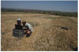
Figure 3. Preparation for the flight. eBee detecting its take-off position by receiving GNSS signals
Figure 4. Monitoring the flight on the ground (25.07.2015)
3.2 Setting Ground Control Points
Establishing ground control points (GCP) provides the model created on tie points with georeferenced and improved relative orientation. Given the fact that the GPS receiver on the eBee’s board is a consumer grade, a few types of errors are expected. They could be errors due to noise in the signal, lack of synchronization between exposition of the camera and the GPS measurement.
Before the flight itself, seven GCPs were put (5 GCPs in the surrounding of the quarry and 2 in the quarry) (see Figure 5. The control points were distributed in relatively same distance between each other in order not to accumulate errors in the model if being close to each other. Most of the GCPs were put on the borders of the quarry. In order for the points to be visible in as many images as possible, the flight lines were extended so that more terrain is captured outside of the quarry. The GCPs coordinates were measured by the aforementioned GPS receiver working with RTK mode using Virtual Reference Station regime.
Figure 5. GCP distribution, image Google Earth
The eBee’s flight resulted in 417 geotagged images. The photogrammetric data was processed with the software Pix4Dmapper. All the 417 images were processed and the achieved Ground Sampling Distance - (GSD) was 3.44cm. As the processing itself takes up to a couple of hours, an experiment with only 209 images was performed, meaning only the images from one flight direction. As a result, the Initial Processing took up to 9min52sec. The achieved GSD in this case was 3.46cm. No matter the reduced number of images, the GSD value was preserved.
3.3.1 Camera Calibration
A really crucial step of the initial processing is the camera calibration. The calibration process optimizes the camera parameters. The software Pix4Dmapper orient the cameras using the keypoint matches. Initially the process is conducted by iterations to restore the camera geometry. The iterations start with taking two cameras only. The calculated camera parameters based on image content only are presented in Table 2 and the radial and tangential distortion in Table 1.
Sensor Width [mm]: 7.40 Sensor Height [mm] 5.60 Focal Length [mm]: 5.20
Table 1. Initial camera parameters of Canon S110 RGB
Sensor Width [mm]: 7.44 Sensor Height [mm] 5.58
Pixel size [µm]: 1.86
Focal Length [mm]: 5.32049 Principal Point x [mm]: 3.80836 Principal Point y [mm]: 2.77957
Table 2. Optimized values of the camera parameters
For precise optimization, the initial camera parameters should be within 5% (0.26mm difference) of the optimized values after the initial process of the images. In the particular case, the difference between the camera parameters before and after is 0.12mm.
By defining the camera parameters, we receive information regarding the radial and tangential distortion of the camera matrix R defines the camera orientation based on the angles
,
and
:
R
Rx Ry Rz
.
.
(2) Let X=(X, Y, Z) is a 3D point in a world coordinate system, then its position in a camera coordinate system X’=(X’,Y’,Z’) is given by:X'RT(XT) (3) The camera distortion model is defined as follows:
Let the point Where r is the image radius from the point xh, yh to the principal point. The distorted homogeneous point in a camera coordinate system (xhd, yhd) is given by:
2 4 6 2 2
The pixel coordinate (xd, yd) of the 3D point projection is given by:
Where f is the focal length and cx, cy are the pixel coordinated of the principal point. (Luhmann, 2014)
Radial Distortion R1: -0.040
Radial Distortion R2: -0.012
Radial Distortion R3: 0.007
Tangential Distortion T1: 0.000
Tangential Distortion T2: 0.004
Table 3. Radial and tangential distortion of the camera lens
Only 6 out of 209 images were not georeferenced (Figure 7.). These are situated in the borders of the flight area. This is due to insufficient image data and overlap. The overlap is essential for the keypoints extraction and matching. Non-georeferenced images are marked in red on the left side of the flight area. The seven ground control points were marked after the initial processing with RMS error of 0.004m. The GSD (Ground Sampling Distance) was used for analyzing the accuracy. In regards to this, the accuracy of the GCPs is less than even one time the GSD = 3.46cm (Table 3).
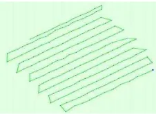
Figure 6. Image positions on the flight strips
Figure 7. Non-georeferenced images marked in red on the left side of the rectangle, indicating the flight area
Theoretically, only three ground control points are needed for the transformation between model coordinate system and geodetic system. Error accumulation in the image matching could be prevented by initiating GCPs at the ends and in the middle of the object as it is in the study case. The accuracy of the GCPs is a biased estimate of the accuracy. Basically, it shows the accuracy of marking the points themselves, not the accuracy of the model after georeferencing. That is why check points are inserted. An end and a middle point were selected for the check control. They were not taken into account for the georeferenced process and optimization. Check points indicate the accuracy of the model. Table 4 shows the accuracy of marking the ground control points. In Table 5 the real accuracy if the model is shown by the two check points.
GCP Number s0XY/Z sX [m] sY [m] sZ [m] GCP110001 0.020/0.020 -0.002 0.004 0.001 GCP110002 0.020/0.020 +0.002 0.000 0.000 GCP110005 0.020/0.020 0.006 -0.004 -0.008 GCP110007 0.020/0.020 -0.002 -0.006 -0.003 GCP110004 0.020/0.020 -0.003 0.008 0.010
Mean [m] 0.000 0.000 0.000
Sigma [m] 0.003 0.005 0.006 RMS Error
[m] 0.003 0.005 0.006
Table 4. Residuals of the ground control points
Point Number s0XY/Z sX [m] sY [m] sZ [m] CP110006 0.020/0.020 -0.009 0.010 -0.036 CP110003 0.020/0.020 -0.025 -0.014 0.020 Mean [m] 0.020/0.020 -0.017 -0.002 -0.008
Sigma [m] 0.008 0.012 0.028
RMS Error
[m] 0.018 0.012 0.029
Table 5. Residuals of the check points
A Point Cloud Densification is the second step of the photogrammetric process and it took 34min57sec. A 3D textured mesh was generated for 15min32sec. This is an essential and compulsory step before getting to volumetric calculation. In conclusion the overall time estimated for the processing of the photogrammetric data was around 1 hour including DSM (Digital Surface Model) and orthomosaic creation (see Figure 8).
Figure 8. Orthomosaic and Digital Surface Model (DSM) of the quarry
3.4 GPS measurements
The GPS measurements were performed the same day of 25 July 2015. A stockpile №4 was measured. The estimated time was one hour and a half. Later the berms of the quarry was
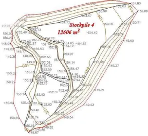
measured for more than 5 hours. The number of points altogether is 615 (Figure 9). The measurement of the stockpile consists of 100 points. Characteristic breaklines were measured to define accurately the real surface of the stockpile. Its boundary was defined by 28 points (Figure 10). After processing, a surface was created in AutoCAD Civil 3D by a group of points and after creation it was defined by 5 contours with one meter interval as shown on Figure 10.
Figure 9. The whole quarry measured by GPS with 615 points for more than 5 hours
Figure 10. Stockpile surface measured by GPS and created in Civil 3D
4 VOLUME CALCULATION
4.1 Calculating the volume of the stockpile from the photogrammetric flight
Basically the principles of calculating the volume of an object in any kind of photogrammetric software, slightly differs from the conventional methods. Unless a Point Cloud Densification is created, Pix4D is unable to compute any volume (Pix4D, 2015). A base surface is needed, so when creating a volume object the stockpile is enclosed by a 3D polylines with vertexes with known coordinates X, Y and Z. The stockpile we are surveying has been enclosed with 59 vertexes (Figure 11). The software creates a grid network of the base surface, for itself, with interval - the value of the Ground Sampling Distance. In the particular case the GSD is 3.46cm/pixel. Volume has been computed cell by cell where the volume of a single cell is given by the equation (1):
. .
i i i i
V L W H , (7)
between the terrain altitude of the cell given in its center and the base altitude in the cell’s center. This expressed in math’s language results in the following equation (8):
Consequently, the volume’s equation for each and every cell could be concluded in the following formula (3):
(9)
Furthermore, it is essential to outline that Pix4D measures a Cut Volume – when the terrain is higher than the base surface, and a Fill Volume – when the terrain is beneath the base.
The total volume of the stockpile is given by the equation (10):
T C F
V V V , (10)
where VT is the total volume of the stockpile VC = Cut Volume
Table 6. Volume calculated in Pix4D from UAV data
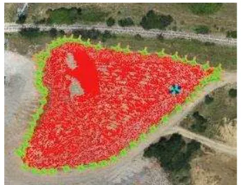
Figure 11. The stockpile enclosed by a 3D polyline
3.1 Calculating the volume of a stockpile from the GNSS measurements
In order to calculate the volume of the stockpile in Civil 3D, a surface has been created from the contours. Contours areas are added together and along with the square root of their product and altogether multiplied by one third of the distance or height between them. This could be simplified by the following equation:
where V = the volume between the two section areas
h = height between the two section areas
A1 = the area of the created surface
A2 = the area of the base line
In practice, having created the surface earlier, we have to select the Stage Storage in the Analyze tab, select Average End Area and Conic Approximation. By this stage of the process a base should be defined which is simply performed by defining a base surface from entities and choosing the created surface of the stockpile. The volume of the stockpile was calculated with a base surface with height Z=150m.The results are the following:
Table 7. Total Volume of the stockpile computed in Civil 3D
4. COMPARISON BETWEEN AND UAV AND GPS VOLUMES
The estimated accuracy of the comparison is up to 3% - 4%. In some countries the legislation states that the volume should be
Expecting no difference in the volumes is not realistic at all as for the different methods of achieving the data. The computed difference is 143.99m3 as the volume from the UAV flight turned out to be a higher value. Large as this difference could seem, when presented in percentage it would be more accurate. As our goal was a smaller difference than 3% which is approximately 382.5m3, the results present a volume difference of 1.1%. In other words, the height difference between the two UAV and GPS surface is 0.032m or 3.2cm. Moreover, the result could state that the height difference between the UAV and GNSS surface is sS= 3.2cm (Cryderman, 2015).
Where
VTthe volume error and S is the area of the reference surface.5. CONCLUSIONS
By this study case, a confirmation of the promising UAV application in stockpile volume calculation was sought. Two values of the volume of the same stockpile were generated as the data was gained by two different methods and consequently processed in a different way. The volume received from the
Total Volume 12 606m3 2
.
.(
Ti Bi)
.(
Ti Bi)
UAV data is 12 749m3 and the volume received from the GNSS points – 12 606 m3. As a result, the UAV volume turned out to be bigger with 144m3. It is more proper to express the difference in percentage which would be 1.1% difference from the whole amount.
It is important to indicate that the UAV data was gathered faster than the terrestrial GPS measurements. The whole area of the quarry was mapped for less than a 30 min in comparison to 5 hours of GNSS measurements. As the image number was reduced, the time for post-process seem to be same.
The achieved accuracy is within the set legitimate error of ±3% which was the main target of the study case. Furthermore, one of the main purposes of the survey is to outline the undisputed application of UAV photogrammetry in the mine engineering. Fortunately, the results of the above study case proves it. Moreover, we should not oversee the fact that UAV technologies would improve drastically, so some future analysis reach better conclusions. To summarize, the paper presented the efficiency and reliability of the unmanned aerial photogrammetry when it comes to volumetric measurements.
6. ACKNOWLEDGEMENTS
The authors are extremely grateful for the support and technical facilities (the eBee and GPS receiver) to Eng. S. Kolev and K. Gizdov.
7. REFERENCES
AUTODESK. 2015. AUTODESK AUTOCAD CIVIL 3D. TO CALCULATE SURFACE STAGE STORAGE VOLUMES. [Online] AUTODESK, 2015. https://knowledge.autodesk.com/. Cryderman, Chris. 2015. Evaluation of UAV Photogrammetric Accuracy for Mapping and Earthwork Computation. GEOMATICA. 2015.
Digital Photogrammetry in the Practice of Open Pit Mining. Patikova, A. 2004. s.l. : ISPRS, 2004. ISPRS. Vols. 34, Part XXX.
Luhmann, Thomas. 2014. Close-Range Photogrammetry and 3D Imaging. 2014.
Mazhrakov, Metody. 2007. Mine Engineering. Sofia : Sofia Univerisity, 2007.
Petrie, Gordon. 2013. Coomercial Operation of Leightweight UAVs for Aerial Imaging and Mapping. GEO Informatics. January/February 2013.
Pix4D. 2015. www.support.pix4d.com. How Pix4Dmapper calculates the Volume? [Online] Pix4D, 2015. https://mapper.pix4d.com/.
SmartBul.Net. 2015. http://www.smartnet.bg/. SmartBul.Net. [Online] 2015.
Surveying a Landslide in a Road Embarkment Using Unammaned Aerial Vehicle Photogrammetry. F. Carvajal, F. Aguera, M. Perez. 2011. s.l. : ISPRS, 2011. Vols. XXXVIII-1/C22.