REDUCTION OF STRIPING NOISE IN OVERLAPPING LIDAR INTENSITY DATA BY
RADIOMETRIC NORMALIZATION
Wai Yeung Yan, Ahmed Shaker
Department of Civil Engineering, Ryerson University, Toronto, Ontario, Canada (waiyeung.yan,ahmed.shaker)@ryerson.ca
Commission VI, WG VII/4
KEY WORDS:LiDAR Intensity, Noise Reduction, Radiometric Correction, Radiometric Normalization, Land Cover Classification
ABSTRACT:
To serve seamless mapping, airborne LiDAR data are usually collected with multiple parallel strips with one or two cross strip(s). Nev-ertheless, the overlapping regions of LiDAR data strips are usually found with unbalanced intensity values, resulting in the appearance of stripping noise. Despite that physical intensity correction methods are recently proposed, some of the system and environmental parameters are assumed as constant or not disclosed, leading to such an intensity discrepancy. This paper presents a new normalization technique to adjust the radiometric misalignment found in the overlapping LiDAR data strips. The normalization technique is built upon a second-order polynomial function fitted on the joint histogram plot, which is generated with a set of pairwise closest data points identified within the overlapping region. The method was tested on Teledyne Optech’s Gemini dataset (at 1064 nm wavelength), where the LiDAR intensity data were first radiometrically corrected based on the radar (range) equation. Five land cover features were selected to evaluate the coefficient of variation (cv) of the intensity values before and after implementing the proposed method. Reduction of cvwas found by 19% to 59% in the Gemini dataset, where the striping noise was significantly reduced in the radiometrically corrected and normalized intensity data. The Gemini dataset was also used to conduct land cover classification, and the overall accuracy yielded a notable improvement of 9% to 18%. As a result, LiDAR intensity data should be pre-processed with radiometric correction and normalization prior to any data manipulation.
1. INTRODUCTION
The use of airborne LiDAR data has progressively increased for surface classification and object recognition (Yan et al., 2015). Despite that, there still exist several knowledge gaps limiting the use of LiDAR intensity data. Among which the striping noise appeared in the overlapping region of mosaicked LiDAR inten-sity data causes undesired disturbance, and such visual detrimen-tal effect undoubtedly degrades the radiometric quality of the data. Regardless of discrete-return or full-waveform LiDAR data, such intensity noise is mainly caused by the signal attenuation due to various system and environmental factors (Jelalian, 1992). Though various correction and calibration techniques have been proposed to reduce the intensity discrepancy based on the use of radar (range) equation (H¨ofle and Pfeifer, 2007; Kaasalainen et al., 2009; Wagner, 2010; Yan et al., 2012), only a few studies ad-dress the striping noise issue when dealing with the overlapping LiDAR data strips.
Luzum et al. (2004) proposed a method to normalize the observed LiDAR intensity by multiplying a dynamic range factor to the power off(f= 2), where such dynamic range factor equals to the range of the observed point divided by a standard range. Such dy-namic range normalization method has been enhanced and used to normalize multiple overlapping LiDAR data strips, particularly for forest canopies, with a notable improvement in terms of clas-sification accuracy (Korpela et al., 2010a,b; Gatziolis, 2011). De-spite that, the method has certain drawbacks which limit its ap-plicability in a universal environment. The selection off (or the two calibration parameters:aandbin (Korpela et al., 2010a,b)) highly depends on the nature of the study site (target character-istics) and the LiDAR sensors (Hopkinson, 2007; Korpela et al., 2010a,b). In addition, the method does not consider other system and environment parameters except the range effect; therefore the method is preferable to be implemented with LiDAR dataset
col-lected for rugged forest terrain within small scan angle (less than 10◦to 15◦). The lack of consideration of incidence angle would
lead to intensity discrepancy, which can be found particularly serious in urban environment with inclined rooftops (Jutzi and Gross, 2010; Abed et al., 2012; Yan and Shaker, 2014). Though there exists preliminary attempts to incorporate Phong model in the radar (range) equation for overlap data strip correction (Ding et al., 2013), Jutzi and Gross (2010) addressed that the Phong model does not really outperform the traditional Lambertian as-sumption in terms of intensity homogeneity.
2. METHOD
2.1 Overall Workflow
Fig. 1 shows the overall workflow of the proposed normalization method. In general, the proposed method can be applied to any entirely or partially overlapping LiDAR intensity data. Firstly, if those system and environmental parameters (i.e. range, scan an-gle, atmospheric attenuation coefficients, etc.) are available, ra-diometric correction can be applied to the original intensity (OI) data (Yan et al., 2012; Yan and Shaker, 2014). Conceptually, the spectral reflectance (or radiometrically corrected intensity (RCI)) is determined for each of the LiDAR data strips (XAandXB) after radiometric correction. Such RCI derived from both LiDAR data strips can be used to generate a joint histogram by searching for all possible pairwise closest points, and a polynomial function is subsequently fitted in the joint histogram. The fitted polyno-mial curve is being treated as an intensity transformation function to normalize the data stripXBwith reference to theXA. After radiometric normalization, the (partially or fully) overlapping in-tensity data strips are interpolated to generate an inin-tensity image. To measure the degree of intensity noise, we compute the co-efficient of variation of selected land cover features and compare the intensity homogeneity between the OI and the radiometrically corrected and normalized intensity data.
Pairwise ClosestPoints XC Intensity bin of XB K
0 LiDARdatastripXA
LiDARdatastripXB Overlap
Polynomial Fitting
Figure 1: Overall Workflow
2.2 Radiometric Correction
Various radiometric correction and calibration techniques have been developed for discrete-return or full-waveform LiDAR data based on the radar (range) equation (H¨ofle and Pfeifer, 2007; Kaasalainen et al., 2009; Wagner, 2010; Jutzi and Gross, 2010; Yan et al., 2012). The purpose of radiometric correction aims to retrieve the surface reflectance of the illuminated object for each of the received laser pulses. As shown in Eq. 1, the radar (range) equation describes the relationship between the received laser power (Pr) with respect to various system and
environmen-tal parameters:
wherePtis the transmitted laser pulse energy, Dr is the
aper-ture diameter,Ris the range,βtis the laser beam width,ηsysis
the system factor, andηatm is the atmospheric attenuation
fac-tor. The laser cross sectionσconsists of the illuminated surface characteristics that can be expressed asσ= 4πρAcosθ, whereA is the projected target area along the direction of the laser beam, θ is the laser incidence angle, andρis the spectral reflectance of the illuminated surface. In Eq. 1, the surface reflectanceρis being treated as the radiometrically corrected intensity data, and the original intensityIis assumed to be directly proportional to the transmitted laser pulsePt. In order to retrieve the surface
reflectanceρ, the aforementioned parameters, if known, can be inputted in the Eq. 1, and those parameters which are unknown
can be assumed as constant. Since effect of overcorrection has been reported when laser incidence angle is used in radiometric correction, a combined use of scan angle and incidence angle can be adopted to resolve such an issue (Yan and Shaker, 2014).
2.3 Radiometric Normalization
After radiometric correction, the intensity data of two partially overlapping LiDAR datasets are used to generate the joint his-togram so as to perform a robust normalization. Unlike geo-referenced image, it is mostly impossible to find a pairwise Li-DAR data point that are situated at the same position in a three dimensional Euclidean space. Therefore, our proposed algorithm has to first locate the closest LiDAR data points from two overlap-ping LiDAR data strips within a threshold distance. The proposed method first utilizes a LiDAR data strip with a larger intensity range as a reference, i.e. XA
={xA1,· · ·, x A a,· · ·, x
A NA}, and
then any LiDAR data strip, i.e.XB
={xB
1,· · ·, xBb,· · ·, xBNB},
with partial/entire overlap can be normalized with reference to XA. For eachxAa ∈XA, we look for the closest point inXB whose Euclidean distanced = kxA
a −xBbk2 is smaller than a
given thresholddmin.yBa thus denotes the resulting closest point
where:
The resultingNC correspondence pairwise LiDAR data points
fromXAandXBare denoted as:
XC={(xAa, yaB)|i= 1,· · ·, NC} (3)
Then, the intensity values of xAa and y B
a are used to generate
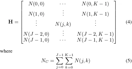
the joint histogramH. JandKare the total number of inten-sity bins of data stripXA andXB, respectively, provided that J≥K.N(j, k)is the number of corresponding pairs of LiDAR data points inXC having intensity valuejinxAa andkinyBa. Therefore, the joint histogramHis a form of aJbyKmatrix:
H=
The intensity transformation function should be in a form of lin-ear relationship or piecewise linlin-ear relationship (Yan and Shaker, 2014). Thus, a polynomial model can be used as an approximate solution to transform the intensity value ofXBtoXA.
3. EXPERIMENTAL WORK
3.1 Study Area and Dataset
proposed approach was examined on two LiDAR datasets col-lected by Teledyne Optech’s sensors. The first dataset, including two data strips, was collected by the Teledyne Optech’s Gemini operating at 1064 nm wavelength. The flight mission was ac-complished on August 24th, 2013, where the air temperature and atmospheric pressure were 20◦C and 1027.4 millibars,
respec-tively. The Gemini sensor was operated with scan frequency 40 Hz, scan angle±20◦, pulse repetition frequency 70 kHz and
fly-ing attitude 1,000 m. With these settfly-ings, the mean point density yields 3.7 points/m2 for the two data strips collected. Table 1
summarizes the LiDAR system settings and data specification.
Table 1: LiDAR system settings and data specification Dataset
Sensor Gemini
Date of Acquisition August 24th, 2013
Number of Data Strips 2
Wavelength 1064 nm
Flying Height ∼1,000 m
Scan Frequency 40 Hz
Scan Angle ±20◦
Pulse Repetition Frequency 70 kHz Mean Point Density ∼3.7 points/m2
Mean Point Spacing ∼1 m
Percentage of Overlap ∼41%
3.2 Implementation
Since the LiDAR data provided were stored inlasformat, thelas
files were first converted into ASCII data format using LAStools. The following fields were read from the las files: x,y,z,I,a, r,n, andtime, where they represent x-coordinate, y-coordinate, z-coordinate, intensity, angle, return, number of returns, and GPS time, respectively. The converted ASCII text files were then im-ported into ArcGIS geodatabase as 3D point features. On the other hand, two individual GPS trajectory files (in 8-byte data format) were read for the two LiDAR datasets in order to re-trieve thexyzcoordinates and GPS time of the aircraft during the flight missions. By interpolating the GPS time of the aircraft and the LiDAR data points, instantaneous aircraft coordinates were computed for each of the data points in the two LiDAR datasets. The range and incidence angle of each LiDAR data point were computed by following the method presented in Yan and Shaker (2014). Then, radiometric correction was applied to all the Li-DAR data strips for both datasets.
In the process of radiometric normalization, a set of pairwise closest points should be first identified in the overlapping region of the two data strips. We used the “Near 3D” tool in ArcGIS to look for the closest pointyaB fromX
B
to pair with axAa from
XA(refer to section 2.3 for detail). As a result of computation, the 3D distance for each pairwise match was computed inXA together with the unique identity of the closest point inXB. Fi-nally, we only selected those pairwise points fromXAandXB with a threshold distance (i.e. dminin section 2.3) less than 5
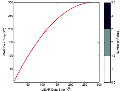
cm. A larger threshold value than that would result in a scattered shape in the joint histogram plot, and thus increases the values in the residual matrixVin Eq.??. The polynomial fitting was implemented in the joint histogram plot, and the coefficients of the polynomial function were computed using MATLAB. Fig. 2 shows the joint histogram plots fitted with a polynomial curve for each of the Teledyne Optech’s datasets. Subsequently, radiomet-ric normalization was applied to the data stripXBin ArcGIS, and then bothXA and normalizedXBwere merged and converted into an intensity image using a 3×3 moving window average method (Reuter et al., 2007).
Figure 2: Joint histogram plot fitted with polynomial function
3.3 Design of Experiments
Two rounds of experiments were conducted on the Gemini datasets in order to test the capability of the proposed method. Firstly, we combined the original intensity data of the two overlapping data strips to form an original intensity image, denoted as OI. We then implemented the radiometric correction and normalization on the two data strips and generated an intensity image, named as RCNI. Apart from visual inspection on the intensity images, a statistical measure, coefficient of variation (cv), was used to assess the in-tensity homogeneity of selected land cover feature (ωi).
cv(ωi) =
σ(ωi)
µ(ωi)
(6)
In this context, a smallercvcorresponds to a less within-class variation of intensity in the land cover sample points. If radio-metric correction and normalization can significantly reduce the striping noise within the intensity data, a reduction ofcvvalue should be recorded.
4. RESULTS AND ANALYSIS
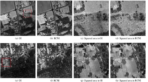
Fig. 3 shows the study area located at the south of the intersec-tion of Highway 48 and Vivian Road. As shown in Figs. 3(a) and 3(e), both OI images had serious striping noise in the cross track direction within the overlapping region. The intensity val-ues located in the bottom half of the image were lower than that of the upper half of the image, resulting in an unbalanced image contrast within the OI. The proposed radiometric correction and normalization successfully removed the striping noise and spikes, and restored the intensity image close to a balanced contrast (see Figs. 3(b) and 3(f)). Despite that, it can be noticed that a low level of striping noise still retained on some of the rooftops in the RCNI.
(a) OI (b) RCNI (c) Squared area in OI (d) Squared area in RCNI
(e) OI (f) RCNI (g) Squared area in OI (h) Squared area in RCNI
Figure 3: LiDAR intensity image of Gemini (1064 nm)
previous two classes, the RCNI still recorded a 19% reduction ofcvin the tree canopies, and a 25% of decrease on the house rooftops. With both visual examination and statistical analysis, the proposed radiometric correction and normalization can sig-nificantly reduce the striping noise appeared in the overlapping region.
Table 2: A comparison ofcvof selected land cover features.
OI RCNI
Bare ground 0.473 0.193 (↓59%) Grass 0.475 0.168 (↓65%) House 0.591 0.443 (↓25%) Road 0.584 0.304 (↓48%) Tree 0.839 0.676 (↓19%)
5. LAND COVER CLASSIFICATION
In order to demonstrate the impact of the striping noise reduction, we used the OI shown in Fig. 3(g) and RCNI shown in Fig. 3(h) to perform land cover classification, and compared their results. As depicted in Figs. 3(g) and 3(h), land cover features including trees, grass cover, paved driveway/road, houses and a warehouse can be found in the study site. Therefore, we identified these five land cover classes for training site selection, and implemented the classification with different combinations of features: 1) in-tensity data only, 2) inin-tensity and digital surface model (DSM), 3) intensity and texture (TEX) features generated from the inten-sity, and 4) inteninten-sity, TEX and DSM. Previous studies reported that the use of entropy texture and homogeneity texture can sig-nificantly contribute to the enhancement of classification accu-racy (Samadzadegan et al., 2010; Huang et al., 2011); therefore, these two texture features were generated for both OI and RCNI with a window size of 9×9 to support the experimental test-ing. A total of eight classification scenarios were implemented by using the traditional maximum likelihood classifier, and 1,000 random checkpoints were generated to assess the classification
results. Table 3 summarizes the overall accuracy generated for all the eight classification scenarios.
Table 3: Overall accuracy of LiDAR data classification results.
OI RCNI
Intensity Only 24.3% 42.4% (↑18.1%) Intensity+DSM 56.0% 65.0% (↑9.0%)
Intensity+TEX 52.8% 69.9% (↑17.1%) Intensity+TEX+DSM 69.3% 83.5% (↑14.2%)
by the reduction of striping noise, and therefore the proposed method should be applied to the overlapping LiDAR data strips before performing any surface classification and object recogni-tion.
6. CONCLUSIONS
This paper presents a radiometric normalization technique to re-duce the striping noise appeared in the overlapping region of air-borne LiDAR intensity data strips. The normalization model is built upon the use of a 2ndorder polynomial function fitted on a
joint histogram plot, which is generated based on a set of pair-wise intensity data points identified within the overlapping Li-DAR data strips. After applying the proposed method on two datasets (Teledyne Optech’s Gemini) with wavelength 1064 nm, the striping noise was significantly reduced in the intensity im-ages. To quantitatively assess the results, we adopted the coef-ficient of variation as a statistical measure to assess the inten-sity homogeneity. The experimental results showed that thecv was reduced by 19% to 65% in the radiometrically corrected and normalized intensity data. We also tested the capability of using LiDAR intensity data to perform land cover classification with different combinations of feature spaces. The results showed that an accuracy improvement ranging from 9% to 18% was achieved in classifying five land cover classes, when the LiDAR intensity data were pre-preprocessed with radiometric correction and nor-malization. The experiments prove that radiometric correction and normalization not only reduce the striping noise visually and quantitatively, but also lead to a notable improvement of overall accuracy when using the intensity data for land cover classifi-cation. The proposed method does not require any selection of parameters or reference targets, and thus overcomes those draw-backs found in the existing normalization techniques based on the dynamic range factor. For large scale seamless mapping, radiometric normalization can be applied to the multiple paral-lel LiDAR data strips with reference to the cross data strip(s). With slight modification, the proposed method can also be imple-mented on mobile LiDAR data and multispectral LiDAR data.
ACKNOWLEDGEMENTS
The research was supported by the Natural Sciences and Engi-neering Research Council of Canada (NSERC) Engage Grant. The authors thank Teledyne Optech Inc., in particular Dr. Joe Liadsky and Dr. Paul LaRocque, for providing the airborne Li-DAR intensity data as well as their constructive comments on the research work.
References
Abed, F. M., Mills, J. P. and Miller, P. E., 2012. Echo amplitude normalization of full-waveform airborne laser scanning data based on robust incidence angle estimation. IEEE Transactions on Geoscience and Remote Sensing 50(7), pp. 2910–2918.
Ding, Q., Chen, W., King, B., Liu, Y. and Liu, G., 2013. Combi-nation of overlap-driven adjustment and phong model for lidar intensity correction. ISPRS Journal of Photogrammetry and Remote Sensing 75, pp. 40–47.
Gatziolis, D., 2011. Dynamic range-based intensity normal-ization for airborne, discrete return LiDAR data of forest canopies. Photogrammetric Engineering & Remote Sensing 77(3), pp. 251–259.
H¨ofle, B. and Pfeifer, N., 2007. Correction of laser scanning in-tensity data: data and model-driven approaches. ISPRS Journal of Photogrammetry and Remote Sensing 62(6), pp. 415–433.
Hopkinson, C., 2007. The influence of flying altitude, beam di-vergence, and pulse repetition frequency on laser pulse return intensity and canopy frequency distribution. Canadian Journal of Remote Sensing 33(4), pp. 312–324.
Huang, X., Zhang, L. and Gong, W., 2011. Information fusion of aerial images and LIDAR data in urban areas: vector-stacking, re-classification and post-processing approaches. International Journal of Remote Sensing 32(1), pp. 69–84.
Jelalian, A. V., 1992. Laser radar systems. Artech House.
Jutzi, B. and Gross, H., 2010. Investigations on surface reflection models for intensity normalization in airborne laser scanning (ALS) data. Photogrammetric Engineering & Remote Sensing 76(9), pp. 1051–1060.
Kaasalainen, S., Hyypp¨a, H., Kukko, A., Litkey, P., Ahokas, E., Hyypp¨a, J., Lehner, H., Jaakkola, A., Suomalainen, J., Akujarvi, A. et al., 2009. Radiometric calibration of Li-DAR intensity with commercially available reference targets. IEEE Transactions on Geoscience and Remote Sensing 47(2), pp. 588–598.
Kim, S. J. and Pollefeys, M., 2008. Robust radiometric calibra-tion and vignetting correccalibra-tion. IEEE Transaccalibra-tions on Pattern Analysis and Machine Intelligence 30(4), pp. 562–576.
Kita, Y., 2006. Change detection using joint intensity histogram. In: The 18th International Conference on Pattern Recognition, 2006, Vol. 2, IEEE, pp. 351–356.
Korpela, I., Ørka, H. O., Hyypp¨a, J., Heikkinen, V. and Tokola, T., 2010a. Range and AGC normalization in airborne discrete-return LiDAR intensity data for forest canopies. ISPRS Journal of Photogrammetry and Remote Sensing 65(4), pp. 369–379.
Korpela, I., Ørka, H. O., Maltamo, M., Tokola, T. and Hyypp¨a, J., 2010b. Tree species classification using airborne LiDAR – Effects of stand and tree parameters, downsizing of training set, intensity normalization, and sensor type. Silva Fennica 44(2), pp. 319–339.
Lu, X., Zhang, S., Su, H. and Chen, Y., 2008. Mutual information-based multimodal image registration using a novel joint histogram estimation. Computerized Medical Imaging and Graphics 32(3), pp. 202–209.
Luzum, B., Starek, M. and Slatton, K. C., 2004. Normaliz-ing ALSM intensities. GeosensNormaliz-ing EngineerNormaliz-ing and MappNormaliz-ing (GEM) Center Report No. Rep 2004-07-01. Civil and Coastal Engineering Department, University of Florida, 8pp.
Mann, S., 2000. Comparametric equations with practical appli-cations in quantigraphic image processing. IEEE Transactions on Image Processing 9(8), pp. 1389–1406.
Pass, G. and Zabih, R., 1999. Comparing images using joint his-tograms. Multimedia Systems 7(3), pp. 234–240.
Samadzadegan, F., Bigdeli, B. and Ramzi, P., 2010. A multiple classifier system for classification of LIDAR remote sensing data using multi-class SVM. In: Multiple classifier systems, Springer, pp. 254–263.
Vain, A., Kaasalainen, S., Pyysalo, U., Krooks, A. and Litkey, P., 2009. Use of naturally available reference targets to calibrate airborne laser scanning intensity data. Sensors 9(4), pp. 2780– 2796.
Vovk, U., Pernuˇs, F. and Likar, B., 2007. A review of methods for correction of intensity inhomogeneity in MRI. IEEE Transac-tions on Medical Imaging 26(3), pp. 405–421.
Wagner, W., 2010. Radiometric calibration of small-footprint full-waveform airborne laser scanner measurements: basic physical concepts. ISPRS Journal of Photogrammetry and Re-mote Sensing 65(6), pp. 505–513.
Yan, W. Y. and Shaker, A., 2014. Radiometric correction and normalization of airborne LiDAR intensity data for improving land cover classification. IEEE Transactions on Geoscience and Remote Sensing 52(10), pp. 7658–7673.
Yan, W. Y., Shaker, A. and El-Ashmawy, N., 2015. Urban land cover classification using airborne LiDAR data: A review. Re-mote Sensing of Environment 158, pp. 295–310.