isprs archives XLI B1 291 2016

2D Sub-Pixel Disparity Measurement Using QPEC / Medicis

M. Cournet a, A. Giros a, L. Dumas b, J. M. Delvit a, D. Greslou a, F. Languille a, G. Blanchet a, S. May a, J. Michel a a

CNES, 18 av Edouard Belin, 31401 Toulouse, France - (myriam.cournet, alain.giros, jean-marc.delvit, daniel.greslou, florie.languille, gwendoline.blanchet, stephane.may, julien.michel)@cnes.fr

b

CS-SI, 5 rue Brindejonc des Moulinais, 31506 Toulouse Cedex 5, France – loic.dumas@c-s.fr Commission V, WG V/4

KEY WORDS: 2D Stereo Matching, Sub-pixel Disparity, Geometric Calibration, QPEC, Medicis

ABSTRACT:

In the frame of its earth observation missions, CNES created a library called QPEC, and one of its launcher called Medicis. QPEC / Medicis is a sub-pixel two-dimensional stereo matching algorithm that works on an image pair. This tool is a block matching algorithm, which means that it is based on a local method. Moreover it does not regularize the results found. It proposes several matching costs, such as the Zero mean Normalised Cross-Correlation or statistical measures (the Mutual Information being one of them), and different match validation flags. QPEC / Medicis is able to compute a two-dimensional dense disparity map with a sub-pixel precision. Hence, it is more versatile than disparity estimation methods found in computer vision literature, which often assume an epipolar geometry.

CNES uses Medicis, among other applications, during the in-orbit image quality commissioning of earth observation satellites. For instance the Pléiades-HR 1A & 1B and the Sentinel-2 geometric calibrations are based on this block matching algorithm. Over the years, it has become a common tool in ground segments for in-flight monitoring purposes. For these two kinds of applications, the two-dimensional search and the local sub-pixel measure without regularization can be essential. This tool is also used to generate automatic digital elevation models, for which it was not initially dedicated.

This paper deals with the QPEC / Medicis algorithm. It also presents some of its CNES applications (in-orbit commissioning, in flight monitoring or digital elevation model generation). Medicis software is distributed outside the CNES as well. This paper finally describes some of these external applications using Medicis, such as ground displacement measurement, or intra-oral scanner in the dental domain.

1. INTRODUCTION

QPEC / Medicis is a two-dimensional sub-pixel disparity measurement algorithm. It was created by CNES (Centre National d’Etudes Spatiales) in the frame of its optical earth observation missions.

This tool can work on a real images pair, but also on a complex images pair (a Synthetic Aperture Radar images pair for instance). This block-matching algorithm is divided into a pixel-wise step and a sub-pixel refinement step, which are described hereafter.

This software is more versatile than most of the computer vision methods found in literature, as it can search the disparity in one-dimensional, but also in two-dimensional. Its 2D search ability is not evaluated here, as most benchmarks are made of stereo-rectified images pairs. But its one-dimensional sub-pixel accuracy is evaluated on a benchmark, called Bergerie1, whose ground truth accuracy is better than a hundredth of a pixel. Its 2D search ability and its sub-pixel accuracy make QPEC / Medicis relevant for CNES activities, such as geometric calibration or performances assessment of earth observation satellites; and for external applications, such as ground displacement measurement and even intra-oral scanner in the dental domain. These CNES activities and external applications based on QPEC / Medicis are described in the two last sections of this paper.

2. QPEC / MEDICIS ALGORITHM

This section details QPEC / Medicis algorithm, at pixel and sub-pixel steps. It also presents some of its match validation criteria.

2.1 General Methodology

Hereafter is a description of the calculations made by QPEC / Medicis, in order to measure the 2D sub-pixel disparity between an images pair. The 2D sub-pixel disparity map is obtained via two major steps, applied on each pixel of the reference image: 2.1.1 A Pixel Step: That consists in calculating the local similarity map at pixel level (local as dedicated to the reference pixel). This local pixel similarity map is obtained by measuring the similarity between the reference window and a set of secondary windows, whose centres are pixels of the exploration area in the secondary image. The maximum of this local similarity map is used to initialise the sub-pixel step (winner-takes-all strategy).

2.1.2 A Sub-Pixel Step: The tool proposes several ways of calculating the sub-pixel disparity. The dichotomy and the iterative optical flow are the ones we focus on:

The Dichotomy: It consists in searching the sub-pixel similarity maximum around the maximum found at pixel level in a dichotomous way.

The number of dichotomous iterations is directly deduced from the precision requested by the user for the disparity measurement (2 iterations for a 0.25 precision, 4 iterations for a 0.1 precision…).

This dichotomous approach can concern either the local pixel similarity map, or the secondary image.

In the first case, the local pixel similarity map is interpolated in the 8 directions around the maximum found at the previous The International Archives of the Photogrammetry, Remote Sensing and Spatial Information Sciences, Volume XLI-B1, 2016

iteration, with a step corresponding to 1/2^n, n being the iteration number (see Figure 1).

Figure 1 : QPEC / Medicis dichotomous approach on the local pixel similarity map. The pixel step, the 1st and 2nd dichotomous sub-pixel steps are here represented.

In the second case, the secondary window is resampled with a fractional shift of 1/2^n in the 8 directions around the maximum found at the former iteration. Then the 8 similarity coefficients are calculated between the reference window and these 8 shifted secondary windows, the new maximum being used to initialise the next iteration.

The Iterative Optical Flow: Once the similarity maximum has been found at pixel step, the secondary window is resampled and centred on it. Then the 2D sub-pixel disparity is estimated in an iterative way by using the shift estimator proposed in (Rais M. et al., 2014). The Rais et al. shift estimator is based on the optical flow shift estimator proposed in (Lucas et al., 1981). At each step, the secondary window is resampled and centred on the 2D translation found at the previous iteration.

2.2 Correlation Window

QPEC / Medicis works with rectangular correlation windows (the windows used are referred to as correlation windows in Medicis, regardless of the similarity measure). The size of the correlation window is defined by its width and length. It can be specified as a constant for all the computed pixels, as an analytic model, or as a correlation window sizes grid. This grid gives the correlation window size for each reference pixel. The idea behind this third possibility is to offer the user the ability to locally adapt the correlation window size to the local texture or to other image features.

2.3 Exploration and Initial Disparity

The exploration area is rectangular; its size is given by the user as a radius in columns and a radius in rows. The exploration center corresponds to the initial disparity given by the user, as a constant for the whole image, as an analytic model, or as an initial disparity grid.

QPEC / Medicis was initially designed for a two-dimensional search and it did not allow the exploration radius to be null in one direction. Since Medicis 11.0 and QPEC 10.0 versions, the search can be done by exploring in a single direction, or even by considering an exploration mask.

A one-dimensional search is indeed relevant for stereo-rectified images, for which the corresponding pixels are on the same image line for both images. In this geometry, exploring in 1D in place of 2D reduces the number of mismatches and saves computational time. This geometry is used for instance in the

Satellite Stereo Pipeline S2P that produces digital elevation models from satellite images (de Franchis et al., 2014a). 2.4 Similarity Measures

Several similarity measures are available in QPEC / Medicis to evaluate the similarity between the reference window and the secondary window.

The most used for real images is the ZNCC (Zero mean Normalised Cross-Correlation).

∑ ̅ .

∑ ̅ ² . ∑ ² (1)

where xi (yi) = pixel value at position i in the reference (secondary) window 1

n = number of pixels in each window

̅ ( ) = mean value of the reference (sec) window The main advantage of the ZNCC is its invariance to a radiometric offset (additive change) and to a positive radiometric gain (multiplicative change) between the two windows. Among the 15 different cost functions evaluated in (Hirschmüller et al., 2009a), the ZNCC is one of the 4 methods of particular interest, even if it presents high errors at discontinuities.

Other similarity measures are also available in QPEC / Medicis for real images. Among them, one can find the Mean Squared Error, the Mutual Information, the Lin K-divergence and the Kullback divergence (Inglada et al., 2007)...

QPEC / Medicis dichotomous approach is also able to work on complex images, such as Synthetic Aperture Radar images. On these complex images, the similarity measure is the coherence, which is the complex ZNCC modulus.

2.5 Measure Sampling and Interpolation

In QPEC / Medicis, the similarity measure is evaluated at integer positions during the pixel step.

For some similarity measures (e.g. Mean Squared Error), this leads to a bad sampling of the measure that can create aliasing on it and that can cause an incorrect estimation of its maximum at pixel step (Szelisky et al., 2004a). If the error is higher than one pixel, this incorrect estimation of the maximum position at pixel step cannot be corrected at sub-pixel step.

Delon et al. showed that the correlation coefficient was also impacted by this risk of incorrect estimation of the maximum position, while evaluating the correlation coefficient at integer positions (Delon et al., 2007a).

Currently, Medicis does not deal with this measure bad sampling issue. Therefore, depending on the images pair and its frequency spectrum, the users either directly use the images; or oversample them (generally by at least a factor 2) and / or apply a low-pass filter on them before using Medicis.

At sub-pixel step, in both cases of the dichotomy (local pixel similarity map resampling or secondary image resampling) and for the secondary window resampling during the iterative optical flow, several interpolators are available: bilinear, optimised bicubic, sinc function apodized by a gaussian, cardinal B-spline.

1

This notation considers the reference window X and the secondary window Y as vectors.

2.6 Validity flags

QPEC / Medicis proposes several match validation criteria, called validity flags. They are summarized in the FLAG VALID and in the FLAG RECAP fields of the Medicis output grid. Below is a short description of the main validity flags available in Medicis.

2.6.1 Correlation Threshold: Two thresholds on the similarity measure at pixel and sub-pixel steps are available. These thresholds can be relevant for the ZNCC, whose value is between [-1; 1]. Experiments show that the difference between the ZNCC value of the maximum at pixel step and the one at sub-pixel step is generally low. Moreover as a high threshold can reject good matches, these thresholds have to be set carefully.

2.6.2 Exploration Area Edge: While setting the exploration area, the user needs to take extra margins. Otherwise Medicis will raise an “exploration area edge” validity flag, for the pixels whose similarity maximum at pixel step is on the edge of the exploration area. This implies that the calculation stops at pixel step for these pixels. If lots of “exploration area edge” validity flags appear in the Medicis output grid, this should warn the user that the exploration area is probably not wide enough (cf 5.1).

2.6.3 Left-Right Consistency: The well-known left-right consistency check is also available in Medicis (Fua, 1993). This test is useful to detect occlusions. It consists in swapping the two images roles (the reference image becoming the secondary image, and vice versa) and in comparing the left-right and right-left disparities sum to a threshold. Usually, the threshold is set

2.6.4 Self-Similarity Threshold: This test can detect ambiguous matches, such as local periodic patterns (Sabater et al., 2012a) or poor textured area (Buades et al., 2015a). It consists in comparing the similarity cost of the best match found during the left-right computation, to the one obtained by performing left-left computation. This last cost is also called self-similarity cost, as it only involves the reference image. For a similarity measure to be maximized (e.g. the ZNCC), the self-similarity flag is raised if (3) is satisfied.

* + ', $ $ ≥ * + ', $ $ (3)

where * + ', $ $ = self-similarity cost = cost of the best match found during the left-left computation

* + ', $ $ = cost of the best match found

during the left-right computation

3. QUANTITATIVE RESULTS ON A SYNTHETIC STEREO PAIR

This section deals with the quantitative evaluation of Medicis on a stereorestitution problem. As stated above, this block matching algorithm makes two-dimensional sub-pixel disparity measurement (without regularization).

However, most disparity measurement benchmarks are based on stereo-rectified pairs, which do not allow a quantitative evaluation of the two-dimensional search ability.

It is the case of Bergerie1 (Sabater et al., 2010), the benchmark that is used in this section. Bergerie1 is a synthetic pair in epipolar geometry, so the 2D search ability of Medicis is not evaluated here. But Bergerie1 ground truth accuracy is about a hundredth of a pixel, which allows sub-pixel error analysis (cf Figure 2 for more details).

Figure 2: Bergerie1 stereoscopic pair and its ground truth. Characteristics of this benchmark: images size: 1024*1024, disparity range in column: [-22, +9], b/h= 0.04 at the centre, ground truth accuracy of about a hundredth of a pixel.

Hereafter are some statistics on the results obtained by Medicis on Bergerie1.

Table 1 presents the impacts on Medicis results of a 1D search, of different sub-pixel methods and of a preliminary oversampling for Bergerie1. Medicis parameters are the default ones, apart from the specified ones in column 1; the correlation window size and the exploration area (cf Table 1 caption). This table presents statistics on the 2D Euclidean distance (called here 2D_Error) between the ground truth and the calculated disparity. The 2D Euclidian distance is here used instead of the error in column, as the calculated disparity in line can be different from zero with the 2D search dichotomy (Dicho2D having a [-2,+2] exploration area in line at pixel step), and with both optical flow options (OptFlow1D2D and OptFlow1D2DZoom2 corresponding to a 2D implementation of the optical flow shift estimator at sub-pixel step).

Medicis options

Table 1: Medicis_V11.0 2D_Error statistics obtained on Bergerie1. Dicho2D corresponds to a 2D search at pixel and sub-pixel steps, and to dichotomy with secondary image resampling for the sub-pixel method. Dicho1D is the same as Dicho2D, but with 1D search at pixel and sub-pixel steps. Dicho1DZoom2 is the same as Dicho1D, but with a preliminary factor 2 oversampling on the input images. OptFlow1D2D corresponds to a 1D search at pixel step, and to the optical flow as the sub-pixel method. OptFlow1D2DZoom2 is the same as OptFlow1D2D, but with a factor 2 oversampling on the input images. Medicis parameters for Dicho2D, Dicho1D, OptFlow1D2D: the correlation window size is 9*9; the exploration area at pixel step is [-22; +10] in column, [-2; 2] in line for the 2D search and 0 in line for the 1D search. Medicis parameters for The International Archives of the Photogrammetry, Remote Sensing and Spatial Information Sciences, Volume XLI-B1, 2016

Dicho1DZoom2, OptFlow1D2DZoom2: both images are oversampled in line and column by a factor 2 before applying Medicis on them; Medicis output grid is calculated with a step in column and line equal to 2; the correlation window size is 19*19 and the exploration area is [-44, +20] in column and 0 in line. Other Medicis parameters for these 5 options: Left-Right consistency and Self-Similarity match validation criteria are activated in their default versions; all other Medicis parameters are the default ones (even for the validity flags). The percentage between brackets corresponds to the density of the Medicis output grid obtained. GTx is ground truth in columns; Dx (resp. Dy) is Medicis disparity in columns (resp. lines), Dy=0 while searching in 1D at pixel and sub-pixel steps, which is only the case for Dicho1D and Dicho1DZoom2.

3.1 Impact of a Search in One-Dimensional

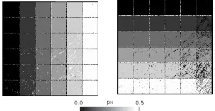
The differences between Dicho2D and Dicho1D in Table 1 are directly linked to the line mismatches that exist in the Medicis 2D search, while working on a pair in epipolar geometry. The minimum exploration radius is 2 while searching in two-dimensional with Medicis; otherwise lots of exploration area edge flags are raised, even when the images are stereo-rectified (cf 2.6.2). On Bergerie1, searching in 1D instead of 2D divides the 2D_Error mean by a factor 1.27 and its maximum by a factor 1.33, but there are still large outliers. Most of these outliers are located on the vertical plane on the right (cf Figure 3). This plane presents a big shear (Sabater et al., 2010), that is not in favor of block matching algorithms.

Figure 3: Dicho1D results obtained on Bergerie1 with Medicis_V11.0: disparity map on the left, validity flags in the middle, error on the right (with error=sqrt[(GTx – Dx)²] as Dy=0 for Dicho1D).

Exploring in 1D instead of 2D also saves computational time. On Bergerie1, Dicho1D is around 3.4 times faster than Dicho2D.

3.2 Impact of the Sub-Pixel Method: Dichotomy vs Optical Flow optical flow approach instead of the dichotomous one increases the 2D_Error mean, but decreases its standard deviation, while the maximum outlier is a little higher.

Medicis options Bergerie1 with several Medicis options that are defined in Table 1. The percentage between brackets in column 1 corresponds to the density of the Medicis output grid obtained (percentage of valid pixels).

Table 2 indicates that the optical flow has better results while considering the valid pixels with an error higher than 1 pixel. But Table 2 also indicates that the dichotomy has better results while considering ¼ pixel or 1/20 pixel errors. The dichotomy indeed matches 72.7% of the pixels with an accuracy better or equal to 1/20 pixel; whereas only 63.4% of the pixels are matched with this accuracy with the optical flow.

As both methods are based on the same 1D local pixel similarity maps, these differences can arise from the impact of match validation criteria and from the sub-pixel step itself.

Both sub-pixel methods have their drawbacks. Regarding the dichotomy, a bad estimation of the maximum during an iterative step cannot be corrected afterward. This could be particularly critical during the first step of 0.5 pixel shift around the maximum found at pixel step. Whereas the sub-pixel shift estimator of the optical flow is currently implemented in two-dimensional, which is penalizing on a stereo-rectified pair like Bergerie1.

On Bergerie1, the computational times of Dicho1D and of OptFlow1D2D are nearly equivalent. But experiments done on large images pairs, with two-dimensional disparity search, show that the optical flow is generally faster than the dichotomy with secondary image resampling by around a factor 4.

3.3 Impact of the Images Oversampling

Last, the impact of a factor 2 oversampling of the images is evaluated on Bergerie1 for both sub-pixel methods: dichotomy and optical flow (Dicho1DZoom2 and OptFlow1D2DZoom2) The original images are oversampled by a factor 2, the output grid is calculated with a step equal to 2 in column and line, the correlation window size and the exploration area in column are doubled. In this case, for each pixel of the original reference image, the 1D local pixel similarity map is calculated with a step equal to the oversampled images step (two times thinner than the step of the original reference image).

Table 1 indicates that oversampling the Bergerie1 images by a factor 2 before running Medicis decreases the 2D_Error mean and standard deviation for both methods.

As indicated in §2.5, this preliminary oversampling limits the

This section describes some CNES applications based on QPEC / Medicis. The first one deals with geometric calibration and performance assessment of earth observation satellites. The second one concerns Digital Surface Model generation. 4.1 Geometric Calibration and Performance Assessment of Earth Observation Satellites

In the frame of several optical earth observation missions, CNES is responsible for the image quality during the in-orbit commissioning and the in-flight monitoring.

QPEC / Medicis has become over the years a key tool for CNES geometric calibration and performances assessment of these satellites. For these applications, the 2D search ability, the sub-pixel accuracy and the preservation of the raw disparity measure can be essential.

Listed below are some CNES activities using QPEC / Medicis in the frame of geometric calibration and performances assessment.

QPEC / Medicis is commonly used for focal plane calibration. This activity consists in defining the viewing directions of each detector of the different retinas. To do so, 2D sub-pixel inter-image correlation is performed (with an external reference for absolute calibration, or with another retina image or another band image for relative calibration). This methodology has been applied on Spot satellites family, on Pleiades HR 1A & 1B (Greslou et al., 2013) and on Sentinel-2 (Languille et al., 2015). The Sentinel-2 Global Reference Image (GRI) production is also based on QPEC. This GRI is then used to ensure the multi-temporal registration of Sentinel-2 products (Déchoz et al., 2015).

In summer 2015, an oscillation anomaly was detected on Sentinel-2. These oscillations were correctly measured on-board, but there was an error in attitude datation. Inter-band correlation via QPEC / Medicis was used to characterise these two-dimensional oscillations and to determine the delay between the image and its corresponding attitude data (Déchoz C. et al., 2015). Solving this anomaly was a pre-requisite to other geometric activities of the Sentinel-2 in-flight commissioning.

4.2 Digital Surface Model generation

Since Spot images, CNES has worked around digital surface model generation.

Spot 1, 2, 3 instrumental focal plane presented for instance a low stereoscopic angle of 0.018 between panchromatic and multispectral bands (Massonnet et al., 1997). Spot 5 HRS instrument was for instance dedicated to the Digital Terrain Model production (stereoscopic angle of 0.8); while the native stereoscopy between panchromatic and multispectral bands of the HGR instrument allowed low stereoscopic angle acquisitions (stereoscopic angle of 0.02) (Vadon, 2003). QPEC / Medicis has been used for the correlation step of the different DSM generation methods developed in CNES since Spot satellites family (Massonnet et al., 1997), (May et al., 2009), (Delvit et al., 2010), (Delvit et al., 2015).

As this tool is not dedicated to DSM generation, the different methods have to improve QPEC / Medicis results to produce better DSM. A multi-scale version of Medicis, including a filtering and a regularization step done at each scale, is for instance detailed in (Delvit et al., 2010). An accurate 100% dense DSM is indeed the grail of DSM generation. So the correlation results need to be filtered to suppress outliers, and interpolated to fill-in holes.

The Figure 4 is an example of 3D point cloud obtained on the Great Pyramid of Giza from Pleiades 1A tri-stereo images. Its quantitative evaluation is given in (Delvit et al., 2015).

Figure 4: Point cloud generated with a Pleiades 1A tri-stereo on Giza Great Pyramid. The correlation step is based on QPEC / Medicis (Delvit et al, 2015).

5. EXTERNAL APPLICATIONS

As above mentioned, Medicis software is distributed outside the CNES as well. This chapter describes two of these external applications using Medicis: ground displacement measurement and an intra-oral scanner.

5.1 Ground Displacement Measurement

In (Rosu et al., 2014a), three two-dimensional sub-pixel correlators are used to measure ground displacements due to seismotectonic events. These two-dimensional correlators are COSI-Corr, MicMac and Medicis.

In this paper, we focus on the preliminary tests done by Rosu et al. on optical satellite images. The secondary image is created by a synthetic displacement of the reference image. The synthetic disparity varies from 0 to 0.5 pixel in columns and lines. The authors present the two-dimensional disparity maps obtained by the three correlators on this pair, while changing the size of the correlation window (9*9 and 33*33).

By using the same Medicis version (Medicis V9.1) and the same Medicis parameters as the one exposed in Table 1 of (Rosu et al., 2014a), CNES did not succeed in finding the same results as the one published by Rosu et al. in Fig 3 and Fig 4. In Table 1 of Rosu et al.’s article, the exploration area is noted 7*3 and there is nothing about the initial disparity.

The authors kindly gave us the parameter file used to obtain the published results (cf Figure 5). It appears that the parameters were the same as in their Table 1, except the initial disparity that was set to 1 in line and -1 in column, and the exploration radius that was set to 2 in line and 2 in columns. That means that the exploration area was in fact [-1; 3] in line and [-3; 1] in column. As the synthetic displacement was from 0 to 0.5 pixel in column and line, lots of pixels had their ZNCC maximum at pixel step on the exploration area edge: +1 in column and less frequently -1 in line. In the Medicis output grid, 9.85% of the pixels were tagged with an “exploration area edge” validity flag, most of them being inside the blocks (cf Medicis validity flags in Figure 6). That means that the maximum at pixel step was on the exploration area edge and that calculations stopped at pixel step for these pixels. This important number of “exploration area edge” invalid pixels inside the blocks points out a trouble in the exploration area. The problem is the same whatever the correlation window size (9*9 or 33*33).

Figure 5 : Medicis 2D disparity map published by Rosu et al.. These maps are obtained with Medicis V9.1 and with the default parameters, except the correlation window (9*9), the initial resemblance threshold (0.6), the final one (0.8), the initial disparity (1 in line and -1 in column) and the exploration radius (2 in line and column). Which leads to an exploration area of [-1 ; 3] in line and of [-3 ; 1] in column, knowing that the synthetic displacement was from 0 to 0.5 pixel in column and line.

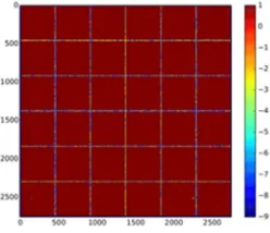
Figure 6 : Medicis validity flags obtained with the same parameters as the one used by Rosu et al. and detailed in Figure 5. The Medicis V9.1 validity flag values are integers included in [-9; 1], 1 representing a valid pixel. 9.85% of the pixels were flagged -2 by Medicis (-2 corresponding to the “exploration area edge” validity flag), which means that the maximum found at pixel step was on the exploration area edge and that the calculations stopped at pixel step. Most of these -2 invalid pixels being inside the blocks, it means that there is a trouble in the exploration area.

With this initial disparity (1 in line, -1 in column) and with an exploration radius of 3, Medicis results on this preliminary test would have been far better than the published ones.

Without initial disparity and with this exploration radius of 2, Medicis results would have been far better than the published ones.

Even with the Medicis default values regarding the exploration radius and the initial disparity (exploration radius of 4, initial disparity of 0), Medicis results would have been far better than the published ones (cf Figure 7). In this case, the exploration area is [-4; 4] in line and [-4; 4] in column. There are around 2.14% of “exploration area edge” invalid pixels that are mainly concentrated in the inter-blocks areas (cf Figure 8).

The reasoning and the conclusions are the same whatever the correlation window size (9*9 or 33*33).

Figure 7 : Medicis 2D disparity map obtained with the same parameters as the one used by Rosu et al and detailed in Figure 5, except the exploration radius and the initial disparity that are kept to the default values (4 for the exploration radius and 0 for the initial disparity). The results are far better than the published ones.

Figure 8 : Medicis validity flags corresponding to the disparity maps presented in Figure 7. There are 2.14% of -2 invalid pixels that are mainly concentrated in the inter-blocks areas (-2 corresponding to the “exploration area edge” validity flag).

With a sufficient exploration area, Medicis results are very close to the synthetic deformation field, except along the river in the case of a 9*9 correlation window size. Some parts of the river are indeed visible on the 2D disparity map obtained with a 9*9 correlation window size (cf Figure 7). A 9*9 correlation window lacks of texture on these parts of the river. As there is neither regularization step, nor multi-scale approach in Medicis, it fails to retrieve the correct disparity on some parts of the river.

As expected, the river is no more visible with a 33*33 correlation window size and the results are smoother (cf Figure 9). This window size is indeed much wider than the river and it realises a smoothing, a kind of regularization of the results.

Figure 9 : Medicis 2D disparity map obtained with the same parameters as the one used in Figure 7, except the correlation window size that is 33*33.

5.2 Intral-Oral Scanner in the Dental Domain

Medicis is also used in a commercial application in the dental domain, as it is embedded in the Condor® optical camera (Pelissier et al., 2016). Condor® is an intra-oral scanner made of two cameras at its extremity.

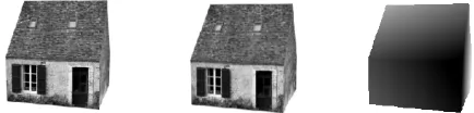
It aims at making 3D optical dental impression that can be used to realise dental prosthesis. The 3D dental impression in colour (cf Figure 10) can also be used by the dentist to explain the diagnostic to a patient or to exchange with a colleague on a case.

Figure 10: On the left: clinical use of the intra-oral scanner Condor®. On the right: 3D dental impression made by this scanner. Medicis takes part in the estimation of its cameras positions.

Medicis takes part in the estimation of the cameras positions of Condor®. When a new image is acquired by the scanner, its disparity with the former images is measured in quasi-real time. Medicis is applied on high gradient areas of the images, in order to improve the two-dimensional sub-pixel disparity measure.

6. CONCLUSION

QPEC / Medicis is a two-dimensional sub-pixel disparity measurement algorithm. It is based on a local method, without regularization.

As shown on the Bergerie1 benchmark, it can present large outliers, but its sub-pixel match accuracy is good. On this benchmark, the 1D dichotomy matches more than 72% of the valid pixels with an accuracy higher than 0,05 pixel.

QPEC / Medicis two-dimensional search ability, coupled together with its sub-pixel measurement ability, is essential in The International Archives of the Photogrammetry, Remote Sensing and Spatial Information Sciences, Volume XLI-B1, 2016

some CNES applications. It is particularly the case for geometric calibration and performance assessment of earth observation satellites.

Its 2D sub-pixel measurement ability is also the reason why Medicis was chosen to be embedded in a commercial intra-oral scanner.

ACKNOWLEDGEMENTS

The authors would like to thank Lionel Moisan for allowing us to use the “Bergerie1” benchmark. We thank Ana-Maria Rosu for kindly giving us the input images and the parameter file used to generate the published Medicis preliminary tests results. We thank Veronique Querbes for the information on Condor®. We are grateful to Hélène Vadon, Claudie Casteras, Damien Pichard, Guillaume Laurent, Carole Amiot and Jonathan Guinet for their past or present work on QPEC / Medicis.

REFERENCES

Buades A., Facciolo G, 2015a. Reliable Multiscale and Multiwindow Stereo Matching. SIAM Journal on Imaging Sciences, Vol. 8, No. 2: pp. 888-915.

http://dx.doi.org/10.1137/140984269.

de Franchis C., Meinhardt-Llopis E., Michel J., Morel J.-M., Facciolo G., 2014a. An automatic and modular stereo pipeline for pushbroom images. In ISPRS Annals of the Photogrammetry, Remote Sensing and Spatial Information Sciences. http://dx.doi.org/10.5194/isprsannals-II-3-49-2014. Déchoz C., Poulain V., Massera S., Languille F., Greslou D., de Lussy F., Gaudel A., L’Helguen C., Picard C., Trémas T., 2015. Sentinel 2 global reference image. Proc. SPIE 9643, Image and Signal Processing for Remote Sensing XXI, 96430A.

http://dx.doi.org/10.1117/12.2195046

Delvit J.-M., Artigues S., 2010. Automatic DEM generation from low B/H stereoscopic acquisition. SPIE 7831, Earth Resources and Environmental Remote Sensing/GIS Applications, 78310J. http://dx.doi.org/10.1117/12.864541

.

Delvit J.-M., L’Helguen C., 2015. Observer la Terre en 3D avec Pléiades-HR. Revue Française de Photogrammétrie et de Télédétection No. 209.

Delon J., Rougé B., 2007a. Small Baseline Stereovision. Journal

of Mathematical Imaging and Vision

Vol. 28, Issue 3, pp 209-223. http://dx.doi.org/10.1007/s10851-007-0001-1.

Fua P., 1993. A Parallel Stereo Algorithm that Produces Dense Depth Maps and Preserves Image Features. Machine Vision and Applications, vol. 6, num. 1, p. 35-49.

http://dx.doi.org/10.1007/BF01212430.

Greslou D., de Lussy D., Amberg V., Déchoz C., Lenoir F., Delvit J.-M, Lebègue L., 2013. Pléiades-HR 1A&1B image quality commissioning: innovative geometric calibration methods and results. Proc. SPIE 8866, Earth Observing Systems XVIII, 886611. http://dx.doi.org/10.1117/12.2023877.

Hirschmüller H., Scharstein D., 2009. Evaluation of Stereo Matching Costs on Images with Radiometric Differences. IEEE Transactions on Pattern Analysis & Machine Intelligence,

vol.31, no. 9, pp. 1582-1599.

http://dx.doi.org/10.1109/TPAMI.2008.221

Inglada J., Muron V., Pichard D., Feuvrier T., 2007. Analysis of Artifacts in Subpiwel Remote Sensing Image Registration. IEEE Transactions on Geoscience and Remote Sensing (Vol-ume:45, Issue: 1) http://dx.doi.org/10.1109/TGRS.2006.882262 Languille F., Déchoz C., Gaudel A., Greslou D., de Lussy F., Trémas T., Poulain V., 2015. Sentinel-2 geometric image quali-ty commissioning: first results. Proc. SPIE 9643, Image and Signal Processing for Remote Sensing XXI, 964306.

http://dx.doi.org/10.1117/12.2194339.

Lucas B. D., Kanade T., 1981. An iterative image registration technique with an application to stereo vision. Proceedings of the 7th international joint conference on Artificial intel-ligence - Volume 2, ser. IJCAI’81. San Francisco, CA, USA: Morgan Kaufmann Publishers Inc., 1981, pp. 674–679. Massonnet D., Giros A., Breton E., 1997. Forming digital eleva-tion models from single pass SPOT data: results on a test site in the Indian Ocean. Geoscience and Remote Sensing. IGARSS '97. Remote Sensing - A Scientific Vision for Sustainable De-velopment., 1997 IEEE International (Volume:2)

http://dx.doi.org/10.1109/IGARSS.1997.615213

May S., Latry C., 2009. Digital Elevation Model Computation with SPOT 5 Panchromatic and Multispectral Images using Low Stereoscopic Angle and Geometric Model Refinement.

IGARSS (4): 442-445.

http://dx.doi.org/10.1109/IGARSS.2009.5417408

Pelissier B., Querbes O., Fages M., Querbes V., 2016. De l’invention de la CFAO à la caméra optique Condor®. Le Chi-rurgien Dentiste de France n°1699.

Rais M., Thiebaut C., Delvit J.-M., Morel J.-M., 2014. A tight multiframe registration problem with application to earth obser-vation satellite design. IEEE International Conference on Imag-ing Systems and Techniques, pp. 6–10 (2014). http://dx.doi.org/ IST.2014.6958436

Rhemann C., Hosni A., Bleyer M., Rother C., Gelautz M., 2011. Fast cost-volume filtering for visual correspondence and be-yond. IEEE Conference on CVPR, pp. 3017–3024.

http://dx.doi.org/10.1109/CVPR.2011.5995372.

Rosu, A.-M., Pierrot-Deseilligny M., Delorme A., Binet R., Klinger Y., 2014a. Measurement of ground displacement from optical satellite image correlation using the free open-source software MicMac. ISPRS J. Photogram. Remote Sensing.

http://dx.doi.org/10.1016/j.isprsjprs.2014.03.002.

Sabater N., Blanchet G., Moisan L., Almansa A., Morel J.-M., 2010. Review of low-baseline stereo algorithms and bench-marks. Proc. SPIE 7830, Image and Signal Processing for

Re-mote Sensing XVI, 783005.

http://dx.doi.org/10.1117/12.865087.

Sabater N., Almansa A., Morel J.-M., 2012a. Meaningful matches in stereovision. IEEE Transaction on Pattern Analysis and Machine Interlligence, vol. 34, no. 5.

http://dx.doi.org/10.1109/TPAMI.2011.207

Szeliski R., Scharstein D., 2004a. Sampling the Disparity Space Image. IEEE Transactions on Pattern Analysis and Machine The International Archives of the Photogrammetry, Remote Sensing and Spatial Information Sciences, Volume XLI-B1, 2016

Intelligence archive. Vol. 26 Issue 3, Page 419-425.

http://dx.doi.org/10.1109/TPAMI.2004.1262341.

Vadon H., 2003. 3D Navigation over Merged Panchromatic-Multispectral High Resolution SPOT5 Images. The International Archives of the Photogrammetry, Remote Sensing and Spatial Information Sciences, 36, 5/W10.