RADIOMETRIC NORMALIZATION OF LARGE AIRBORNE IMAGE DATA SETS
ACQUIRED BY DIFFERENT SENSOR TYPES
S. Gehrke a, B. T. Beshah b
a
Hexagon Geosystems, Leica Geospatial Solutions Division, Goethestr. 42, 10625 Berlin, Germany – [email protected]
b
North West Geomatics Ltd., 245 Aero Way NE, Calgary, AB T2E 6K2, Canada – [email protected]
Commission I, WG I/4
KEY WORDS: Multi-Sensor, Aerial Images, Sensor, Radiometry, Radiometric Adjustment, Mosaic
ABSTRACT:
Generating seamless mosaics of aerial images is a particularly challenging task when the mosaic comprises a large number of im-ages, collected over longer periods of time and with different sensors under varying imaging conditions. Such large mosaics typically consist of very heterogeneous image data, both spatially (different terrain types and atmosphere) and temporally (unstable atmo-spheric properties and even changes in land coverage).
We present a new radiometric normalization or, respectively, radiometric aerial triangulation approach that takes advantage of our knowledge about each sensor’s properties. The current implementation supports medium and large format airborne imaging sensors of the Leica Geosystems family, namely the ADS line-scanner as well as DMC and RCD frame sensors. A hierarchical modelling – with parameters for the overall mosaic, the sensor type, different flight sessions, strips and individual images – allows for adaptation to each sensor’s geometric and radiometric properties. Additional parameters at different hierarchy levels can compensate radiome-tric differences of various origins to compensate for shortcomings of the preceding radiomeradiome-tric sensor calibration as well as BRDF and atmospheric corrections. The final, relative normalization is based on radiometric tie points in overlapping images, absolute radiometric control points and image statistics. It is computed in a global least squares adjustment for the entire mosaic by altering each image’s histogram using a location-dependent mathematical model. This model involves contrast and brightness corrections at radiometric fix points with bilinear interpolation for corrections in-between. The distribution of the radiometry fixes is adaptive to each image and generally increases with image size, hence enabling optimal local adaptation even for very long image strips as typi-cally captured by a line-scanner sensor.
The normalization approach is implemented in HxMap software. It has been successfully applied to large sets of heterogeneous imagery, including the adjustment of original sensor images prior to quality control and further processing as well as radiometric adjustment for ortho-image mosaic generation.
1. INTRODUCTION
The generation of radiometrically homogeneous image mosaics requires global and local radiometric adjustment. In the context of this paper, this adjustment is the final step of a radiometric image correction chain: the relative normalization to achieve practically seamless mosaics. The generation of seam-lines for ortho-image mosaicking is described in a companion paper by Al-Durgham et al. (2016).
1.1 Motivation
The task of relative radiometric normalization becomes an especially challenging one with increasing complexity or, res-pectively, diversity of the input data. Large data sets typically imply different types of terrain with very different reflectance properties as well as varying atmospheric conditions – along with spatial and temporal changes in illumination and viewing geometry. They are often captured using a number of different sensors. Furthermore, re-flights have to be integrated with the original imagery. For most data sets, even the larger ones, the majority of radiometric differences is greatly reduced by sensor calibration and subsequent atmospheric and anisotropic ground reflectance corrections. However, considering the variety of potential sources of radiometric ‘error’ in combination with the limitations of correction models (see section 2), it becomes apparent that sometimes significant radiometric differences can
remain for complex mosaicking scenarios. An example is illus-trated in Figures 9 and 10. Such differences are to be removed by the final radiometric normalization step.
The authors have designed and implemented a relative radio-metric normalization for Leica ADS imagery, which is the last part of the correction chain in ortho-image mosaic generation (Downey et al., 2010; Gehrke, 2010). For the very long ADS image strips, a location-dependent radiometry model is used, based on low-order polynomial correction functions for image contrast and brightness, which allow for spatial variation along strip. Correction coefficients are computed in a least squares solution for the entire mosaic, based on radiometric tie points in overlapping image areas that are to be adjusted. While this approach is able to deliver satisfactory results for most ADS mosaics, some larger projects – such as the radiometric norma-lization of entire states in the U.S. – have meanwhile revealed its limitations: Low-order polynomials (typically quadratic) have been identified as too rigid and too coarse in some cases; respective mosaics still show localized radiometric differences after normalization that would not meet production standards and user specs (cp., e.g., Figure 6).
Another issue of our initial approach is an occasionally evident dynamic range reduction. This is partially inherent to (many) radiometric normalization methods but also amplified towards the ends of the ADS strips by the polynomial model. Finally, larger remaining differences between images from different sessions have been observed, especially in case of re-flights.
These findings were the main driver to develop a refined ap-proach that allows for more localized adaptation of radiometry while also becoming more robust, essentially by integrating knowledge about the sensor, the flight configuration and the entire data processing chain.
1.2 Goals
The main goal of a radiometric normalization can be put very concisely: no visible transitions between overlapping images. In addition to this local adjustment, the option of a global homo-genization throughout the mosaic is desired. With regard to the ADS, a location-dependent parameterization is crucial, capable of modeling radiometric variations within only a few 1,000 image pixels.
The normalization approach has to be applicable to the imagery of different types of airborne sensors of the Leica Geosystems family, currently the Leica ADS line scanners as well as DMC large-format frame and medium-format RCD nadir and oblique sensors. To achieve optimal results, it is especially desired to utilize the knowledge about geometric and radiometric sensor properties, imaging configuration, flight pattern and data pro-cessing, including the characteristics and also the limitations of preceding radiometric corrections. The functional model and its implementation need to be expandable for future developments, providing a well-defined interface to, e.g., add a new type of sensor.
While ADS view angles vary only across-strip, the viewing geometry of frame sensors is different for all image pixels. Including oblique views, the very large range of zenith angles results in significant radiometric inhomogeneity. Therefore, it is desired to compute radiometric corrections including relative normalization early in the processing chain. This is carried out at the time of ingesting a flight session and, accordingly, applied to the images in their original geometry. Based on that, calibra-ted and homogeneous imagery is available for quality control and throughout further processing.
In case of ortho mosaic generation, the options of introducing reference images from neighboring blocks or radiometric con-trol points should be provided. Instead of mosaic homogeniza-tion in itself, the overall radiometry must be adjusted towards the reference in this case. Along the same lines, it is desired to adjust a mosaic consecutively. The main practical use cases are adding re-flight images to an existing mosaic and adjusting data from oblique views to a nadir reference.
However, the main (current) application is the normalization without radiometric control or reference mosaic. In this case it is required to retain the average radiometry of the input images with regard to color, brightness and – based on the experience from using our initial approach – especially dynamic range. It is noteworthy that the latter is a general challenge for most radio-metric normalization approaches.
1.3 Recent Developments in Radiometric Normalization
Relative radiometric normalization has been a research topic for decades, predominantly in the field of satellite imagery, but, more recently, also for the adjustment of aerial image mosaics. In that context the block-wide radiometric normalization is often called ‘radiometric aerial triangulation’ because of various similarities to a geometric aerial triangulation.
Surveys on radiometric normalization approaches can be found in, e.g., Yang and Lo (2000), Over et al. (2003), Hong (2007), Gehrke (2010) and Pros et al. (2013), which discuss and, in parts, compare approaches for histogram adaptation, retrieval and evaluation of radiometric tie points (‘invariant features’) as well as computational aspects. radiometric corrections into one, Chandelier and Martinoty (2009), Gonzales-Piqueras et al. (2010), Lopez et al. (2011) and Pros et al. (2013) combine atmospheric and/or BRDF models with the normalization under consideration of radiometric tie points. The resulting mosaics presented by Chandelier (2009) and Lopez (2011) suggest that the BRDF models used in their combined radiometric adjustments might not fulfill our require-ments, particularly not in case of ADS image strips from differ-ent sensors and flight sessions. Even though the shortcomings should be overcome by additional degrees of freedom, we do not see a benefit in integrating different types of corrections into one compared to computing them subsequently. This approach has been taken by Downey et al. (2010) and Gehrke (2010) for ADS and also by Pagnutti et al. (2015) for DMC. It is important to note that in both cases corrections are applied and, most important, chained on the fly, so the very imagery is modified only once (cp., e.g., Downey et al., 2008).
The separation of radiometric corrections provides the oppor-tunity to collect radiometric tie points for the final relative normalization step with atmospheric and BRDF corrections applied, which allows for more robust removal of outliers. Pro-cedures for tie point evaluation have been investigated in detail in the context of our initial radiometric normalization (Gehrke, 2010). There are essentially two kinds of automatic approaches to retrieve a representative and well-distributed set of radio-metric tie points for the normalization of large mosaics: sampling in a (regular) grid with subsequent evaluation (e.g.: Chandelier and Martinoty, 2009; Gehrke, 2010; Pagnutti et al. 2015) or re-use of geometric tie points from aerial triangulation (discussed in Lopez et al., 2009) or more homogeneous patches near-by (Pros et al., 2013). Based on the outlier elimination as part of a geometric triangulation solution, the second approach provides geometrically corresponding points while the first is more generic and can be applied without geometric triangu-lation. However, especially in this case it requires more robust outlier elimination. In addition to our initial evaluation pro-cedures, we consider the work of Pagnutti et al. (2015) in that regard.
As pointed out in the introduction of this paper, the spatial para-meterization by polynomials as used by Gehrke (2010) and also by Falala et al. (2008) and Molina et al. (2011) is not sufficient for ADS. A more localized model is used in geometric triangu-lation of line-scanner images, based upon so-called orientation fixes with linear or non-linear interpolation of corrections to the exterior orientations in-between (Hinsken et al., 2002; Gruen and Zhang, 2003; Gehrke and Beshah, 2013). Such an approach can be transferred to radiometric modeling.
2. THE HXMAP IMAGE CORRECTION CHAIN
The relative normalization is the final step of the radiometric processing chain, required to remove remaining differences left after the removal of atmospheric and BRDF effects. Therefore, the correction models provided in Leica Xpro and/or HxMap software – and especially their (partially desired) limitations – are briefly discussed here for ADS and DMC image processing.
2.1 Aerial Image Formation and Correction
The amount of radiance collected in an imaging sensor is affected by anisotropic reflectance of the observed ground, by
the atmosphere and by the sensor itself. All of which effects are usually undesired. They need to be corrected when aiming for calibrated and homogeneous reflectance images.
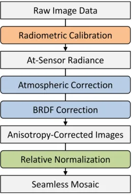
Radiometric properties of the sensor optics and electronics can be calibrated in the laboratory and corrected with high preci-sion. Capturing, modeling and, accordingly, correcting the bi-directional reflectance (BRDF) of different ground materials as well as the atmospheric impact is, to a degree, approximate (see, e.g., Beisl et al., 2008, or Pagnutti et al., 2015). Therefore, the final relative normalization is applied, which leads to the radio-metric correction chain illustrated in Figure 1.
Figure 1. Radiometric correction work-flow for aerial images.
There exists a number of BRDF and atmospheric models with different complexity, which can be empirical or physical. They generally consider illumination and viewing geometry, which is well-known in our case.
2.2 Leica DMC Frame Corrections
The viewing geometry of frame images is different for each individual pixel, which means the atmospheric and BRDF im-pacts vary accordingly. Therefore, a correction retrieved from individual frame images will generally not deliver optimal results. A more advanced computation for DMC is based on combining multiple frames with comparable reflectance pro-perties, i.e. similar view angles and little temporal difference. These are usually the images captured subsequently in a flight strip.
The correction for atmospheric haze is carried out by dark pixel subtraction independently for each image band, with dark pixels collected in a two-dimensional grid from multiple frames. A subsequent gradient correction removes the view-angle-depen-dent impact of atmospheric path lengths as well as anisotropic reflectance effects, separately for land and water areas. The computation approaches for both types of corrections are based on Pagnutti et al. (2015).
2.3 Leica ADS Line-Scanner Corrections
As for all line-scanning sensors, the view angles for the ADS are practically constant along strip and vary only across. With our current models assuming constant illumination angles – i.e. ignoring the (slight) change of sun angles during the scan of a single strip –, atmospheric and BRDF corrections for ADS be-come one-dimensional models, applied throughout each image strip.
There is a number of atmospheric correction models of different complexity available for ADS, namely dark pixel subtraction, ‘Modified Chavez’ as well as the ‘Modified Song-Lu-Wesely’ method. The latter is based on solar position, flying height, ground elevation and viewing geometry; it also considers as dark pixel radiance from image statistics (Beisl et al., 2008; Downey et al., 2010). The BRDF correction for ADS is based on statistics for the land surface of the whole image. It utilizes the ‘Modified Walthall’ model, which includes a hot spot term (Beisl et al., 2006).
2.4 Model Limitations
Both the ADS across-strip corrections and the multi-frame corrections imply stable atmosphere throughout the strip. Fur-thermore, atmospheric path lengths are assumed to be constant (per view angle), which is not the case, e.g., in mountainous terrain. The along-strip changes in illumination and viewing geometry, even though generally small, are averaged out in all of our atmospheric and BRDF models.
Since the radiometric models are generally empirical or semi-empirical, they do not fully model all atmospheric and BRDF impacts (which is practically impossible). In particular, BRDF corrections do not consider slope, which does locally affect the reflectance geometry. In that regard, the image resolution is a limiting factor, too, because anisotropic reflectance largely de-pends on sub-pixel surface structure. See Beisl et al. (2008) for a more detailed discussion on such model limitations. Finally, a BRDF is a property of a particular material, and its (current) generalization to all types of land coverage averages out any differences.
It is important to note that some of these model limitations and approximations are desired in order to provide robust radio-metric corrections for a large variety of data sets from different sensors and image resolutions. The models are still capable of correcting the vast majority of anisotropic reflectance and atmo-spheric effects, which is readily illustrated in Figure 4. How-ever, remaining radiometric differences have to be normalized to achieve homogeneous mosaics. According to the discussion above, predominantly along-strip effects need to be corrected for. In addition to that, a certain level of overall disagreement between flight sessions can be expected, if those are captured under dissimilar atmospheric conditions and/or by different sensors.
3. RADIOMETRIC NORMALIZATION APPROACH
The radiometric normalization as described in the following is based upon Gehrke (2010). Most significant improvements compared to this initial approach are the new location-de-pendent parameterization using radiometry fixes, more robust evaluation of radiometric tie points (see section 4) and the hierarchical modeling approach, applicable to ADS and frame sensors.
3.1 Histogram Adjustment
As discussed in the introduction of this paper, radiometric corrections for the relative normalization step follow a linear histogram adaptation model, consisting of contrast c (scale factor) and brightness b (offset) – see section 1.3 and also Gehrke (2010). Thus, any input DN is corrected according to the following equation:
Note that more complex, non-linear models would be possible, but the benefit is considered minor. Far more important is the computation and application of location-dependent contrast and brightness parameters.
For multi-spectral images, the histogram adaptation needs to be carried out per band. The normalization is either relative, i.e. averaging but inherently not altering the overall mosaic radio-metry, or it is based on reference images and/or radiometric control points with the same number of bands as the mosaic. Accordingly, it can be computed and applied for each band independently without causing undesired color shifts.
3.2 Radiometry Fixes
Both relative radiometric normalization – or radiometric aerial triangulation – and geometric aerial triangulation have to pro-vide means of location-dependent parameterization for the long ADS image strips. In the geometric case, a common approach is defining a number of orientation fixes along strip, for which corrections to the initial exterior orientation are computed in the triangulation adjustment. Any correction in-between orientation fixes is interpolated using linear or non-linear functions (cp. Hinsken et al., 2002; Gruen and Zhang, 2003; Gehrke and Beshah, 2013).
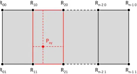
This orientation fix approach can be transferred to radiometric normalization, modeling contrast and brightness corrections each in a grid of radiometry fixes as illustrated in Figure 2. An image then features m x n radiometry fixes, typically n = 2 for ADS (across-strip) and n = m = 2 for frame, i.e. radiometry fixes in each image corner.
Figure 2. Typical radiometry fix layout for an ADS image, with bilinear interpolation of the correction parameters at point Pxy.
For each image location Pxy, the normalization corrections for contrast, cxy, and brightness, bxy, are bilinearly interpolated between respective parameters, cij and bij, at the neighboring radiometry fixes, Rij (Figure 2). Note that, for simplification, radiometry fix indices of the bilinear mesh start at 0 in the equation below. Similarly, the interpolation coordinates Δx and Δy refer to the upper-left radiometry fix involved in the
com-Contrast and brightness corrections at the radiometry fixes are computed in the normalization adjustment as described in sec-tion 3.4.
3.3 Hierarchical Parameterization
The order of magnitude of the contrast and brightness correc-tions required for relative normalization can vary significantly within a mosaic. Furthermore, it can be expected to generally increase with mosaic size as large mosaics combine image data with considerable spatial and temporal differences. Both of which generally amplify the radiometric differences left after sensor calibration and atmospheric and BRDF corrections as discussed in section 2.
Optimal parameterization for radiometric normalization should account for the (potential) source of the differences it is expec-ted to compensate. This means it needs to take into account the hierarchical structure of a mosaic: The smallest unit is a single frame or, respectively, an ADS image strip. Radiometric dif-ferences along the latter are handled by the radiometry fix approach. For the first, radiometry fixes would still allow to correct remaining gradients along and across individual frames – which can occur since all images of a frame image strip are pre-corrected based on the same atmospheric and BRDF para-meters. To compensate along-strip differences, additional cor-rection deltas for each image should be introduced. The same applies at strip level, considering the underlying multi-frame corrections are common per strip. (Note that in case of the ADS image and strip are essentially the same in the context of mo-saicking.)
The largest amount of radiometric differences most probably occurs in-between flight sessions; an example of which is discussed in section 5.4. This can and should be accounted for by introducing correction deltas at session level and, along the same lines, at sensor level in case different types of sensors have contributed to the mosaic. The resulting contrast and brightness correction equations are still based on radiometry fixes, extended by the aggregated deltas at different hierarchy levels:
Parameterizing common radiometry changes at higher levels, especially for the flight sessions, results in a certain amount of global mosaic homogenization without explicitly forcing it as initially carried out by Gehrke (2010).
The hierarchical parameterization is an extension of the BMSI (block, mission, strip, image) modelling by Mulawa (2000). Even though the equations are (currently) used for both ADS and frame sensors the same way, the concept allows for sensor-specific modifications or additions at different levels. Adding a new type of sensor into the radiometric normalization adjust-ment is carried out by impleadjust-menting the hierarchical interface. This concept is described in more detail by Gehrke and Beshah (2013) for a geometric aerial triangulation.
3.4 Global Least Squares Solution
The radiometric normalization parameters for all images in the mosaic are computed simultaneously in a least squares adjust-ment. This adjustment is based upon the DNs of radiometric tie points in all image overlaps (see section 4). Radiometric dif-ferences between overlapping images are eliminated by forcing the equality of the adjusted DNs of any given point that ties these images. Corrections for the very tie point location (x,y) in
each image are interpolated in the respective grid of radiometry fixes (section 3.2), with higher-level correction deltas added (section 3.3). This leads to the main observation equation, one for each radiometric tie point in the mosaic:
To avoid the trivial but undesired solution, c = 0, the adjustment needs to be constrained, e.g., by adding the following conditions for the correction parameters at all radiometry fixes, Rij, of all images:
And, similarly, for the correction deltas of different hierarchy levels:
Weighting between these conditions and the observation equa-tions controls the amount of (potential) radiometric change at different levels in the hierarchy. If too rigid, differences can not be adjusted as desired; if too loose, dynamic range could be reduced significantly. Unfortunately, an average loss of dyna-mic range is inherent to radiometric normalization based on the equation system presented so far – and considered a potential risk of comparable approaches of, e.g., Falala et al. (2009) and Gehrke (2010); for the latter, this effect was pointed out as an evident drawback earlier in this paper.
With the new hierarchical parameterization, such an effect is en-tirely avoided by constraining the average corrections of the n x m radiometry fixes per image as follows:
This is modeled as a hard constraint (with strong weight), which practically means the radiometry fixes allow for local adaptation within each image, but they do not alter the overall images in each sensor type and, finally, the sensor type corrections at the mosaic level. This approach is essentially a free network adjust-ment, retaining the ‘radiometric datum’. As a result, the mosaic will be adjusted where required but the overall radiometry is not
systematically modified; there is especially no reduction of the (average) dynamic range.
With the introduction of reference images or radiometric control points the ‘radiometric datum’ is defined and the above cons -traints can be omitted to allow for adaptation to the reference. The observation equations for adjusting an image to a reference image it overlaps are as follows, as above based on radiometric tie points:
A mosaic with reference images consists of two types of obser-vation equations, depending on the role of images in a particular overlap. Reference images can be introduced from neighboring mosaics that are already normalized, so seamless transitions are achieved. Other examples are fitting individual re-flight images into an existing mosaic or adjusting oblique images to a nadir reference. In both cases the initially normalized images act as reference images in subsequent steps.
Radiometric control points (or patches) can be introduced into normalization similar to reference images – with the difference that target DNs are located in the respective image itself, in-dependent from overlap.
4. RADIOMETRIC TIE POINTS
The collection, evaluation and thinning of radiometric tie points is described in detail by Gehrke (2010). Since then, the method has been generalized to define the tie point pattern in object space. Minor additions have been made to provide an even more robust tie point evaluation, which is beneficial especially for mosaicking original sensor images.
4.1 Data Collection
Tie points are used to adjust radiometric differences between overlapping images. The area of interest for point collection is the entire overlap. Points are collected in a regular grid in object space with a spacing that provides enough points, so that sub-sequent evaluation, blunder elimination and thinning result in a representative, well-distributed set of points.
Based on the known image or sensor geometry and orientation, tie point candidates are projected into each image of the over-lapping pair. As investigated by Gehrke (2010), collection can take place in minified overviews of the imagery, which also means the accuracy of a global elevation model (e.g., SRTM) is usually sufficient to retain co-location in the original sensor images – with exceptions, e.g., in mountainous areas. Potential mismatches need to be eliminated as described below. However, this is not an issue for ortho-rectified mosaics.
It is desired to collect points from radiometrically homogeneous areas, so the DNs for tie points are retrieved in a small window. The final DN for each image is the respective window average, provided the window DN standard deviations are within a specified threshold.
4.2 Evaluation and Thinning
To provide invariant (identical) features for normalization, the sampled tie points undergo several consistency checks based on statistical methods and classification. These include the relative difference of the DNs from overlapping images, across-band correlation, water elimination (if desired) and blunder elimina-tion considering the normalizaelimina-tion equaelimina-tions.
The cross correlation between the tie point DNs of all bands of a pair of images A and B, normalized by the respective DN
rage across bands, is provided by Scheidt et al. (2008), with a threshold of C > 0.8:
Depending on the application and also on prior radiometric cor-rections, water areas might need to be eliminated from normali-zation. Tie points collected in water areas can be classified based on the Normalized Differenced Vegetation Index (NDVI) or, with largely similar results, the Normalized Differenced Water Index (NDVI) according to McFeeters (2006).
For calibrated imagery, practical thresholds that indicate water pixels are in the order of NDVI < 0.1 and NDWI > 0.2. In theory, further evaluation of radiometric tie points – namely blunder detection – would be provided by the global least squares adjustment itself. However, the system of equations is generally large for large mosaics (there can be millions of tie point observations), which would impact the performance of such a robust solution. But a very similar result in terms of tie point elimination is achieved when working with individual overlaps, where the number of tie points is comparatively small. Based on the idea of Pagnutti et al. (2015), such a blunder elimi-nation can be carried out by adjusting one image in the overlap to the other, which acts as a reference in this computation (see section 3.4), without any constraints or higher-level parameters involved. Blunder points are iteratively identified and removed by Data Snooping (Baarda, 1968).
For all statistical criteria for tie point elimination one needs to bear in mind that the goal is the removal of only gross errors while retaining a broad range of tie point DNs. Thus, the level of ‘radiometric accuracy’ assumed in this context is rather low. We found that a useful standard deviation for an individual DN is 10 % of the image average, applied in Data Snooping and also for the global mosaic adjustment.
Tie points remaining after the evaluation steps – typically the vast majority – are finally thinned in such a way that every im-age overlap is divided into a grid. Based on the desired amount, tie points are randomly selected within each grid cell to ensure an even distribution. See Gehrke (2010) for an investigation on the number of points and their effect on normalization results.
5. RESULTS FROM DIFFERENT SENSORS
The new radiometric normalization is part of HxMap, applied to the airborne sensors of the Leica family. Results are shown for ADS and DMC, including an example of all subsequently ap-plied radiometric corrections.
5.1 Evaluation of Normalization Results
Since the main objective of the radiometric normalization is the seamless mosaic, visual inspection of the correction result at global and local scales becomes the decisive criteria for quality control. This assessment is supported quantitatively by the DN
differences in radiometric tie points before and after adjustment, for individual image overlaps and also globally. Their averages should be very close to 0, RMS values are expected to reduce, roughly to the level of the initial DN difference standard devia-tion.
Even though an overall reduction of dynamic range is inherently prevented, it can still happen locally in case of too many outliers in radiometric tie points or incorrect weighting between DN difference observations and conditions in the adjustment. There-fore, the resulting correction parameters need to be verified, both individual contribution deltas at different hierarchy levels and aggregated values.
5.2 Full Correction Chain for a DMC Flight Session
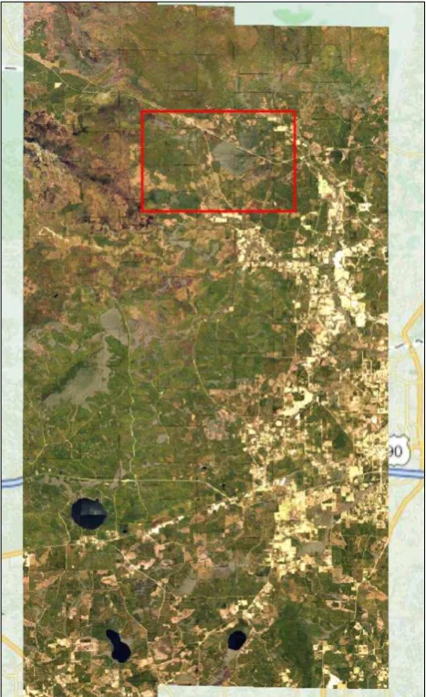
The individual steps of the radiometric correction chain are best illustrated for a data set that has been flown at high altitude, so there is significant atmospheric impact to correct. Such an example is Baker County, Florida, which has been imaged with a DMC II 250 sensor by Quantum Spatial (Photoscience) in 2014. Flight altitudes are almost 6,000 m above ground, resul-ting in a GSD of 0.30 m. The session consists of 314 images in 9 strips, flown North-South. The final radiometry is shown in Figure 3 as a session overview; Figure 4 compares the contribu-tions of individual correction steps.
Figure 3. Overview of a DMC-II flight session in Baker County, Florida, with all radiometric corrections applied. The rectangle marks the area of Figure 4.
Figure 4. DMC radiometry correction chain for a sub-section of Baker County. From top to bottom: imagery after subsequent sensor calibration, dark pixel subtraction, gradient correction, and final radiometric normalization.
The Baker County data set nicely illustrates the capabilities and also the need of applying radiometric corrections: The dark pixel subtraction successfully removes the predominantly bluish haze component; the gradient correction eliminates the vast majority of remaining differences. It leaves only very few recognizable seams between the images, most obvious in the central part of the area shown in Figure 3. This difference is adjusted in the radiometric normalization.
5.3 Example of Water Normalization
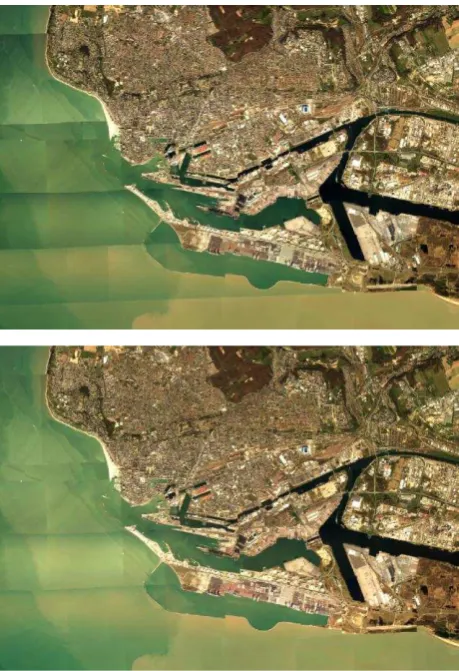
DMC multi-frame gradient correction models are computed and applied separately for land and water areas. Therefore, the final normalization explicitly includes water in the mosaic adjust-ment. A particularly challenging example with distinctly dif-ferent water areas is shown in Figure 5.
This DMC II 250 session, consisting of altogether 606 images in 23 strips, has been provided by APEI (France). It covers the French city of Le Havre, which is located at the estuary of the river Seine (Southern part of the imagery) into the English Channel (in the West). Including the canals of the port of Le Havre, the appearance of water is distinctly non-uniform, which leaves significant radiometric differences after the strip-based water gradient correction (Figure 5, top). The radiometric nor-malization is capable to reduce this effect but – inherent to its approach – fails to compensate non-linear gradients that predo-minantly occur across the images in some of the strips (Figure 5, bottom).
Note that also the land part is slightly improved by radiometric normalization; areas around the city center become more even.
Figure 5. Radiometric normalization of heterogeneous water areas in Le Havre, France. Top: imagery after gradient cor-rection; bottom: final normalization result.
5.4 The Benefit of Radiometry Fixes for ADS
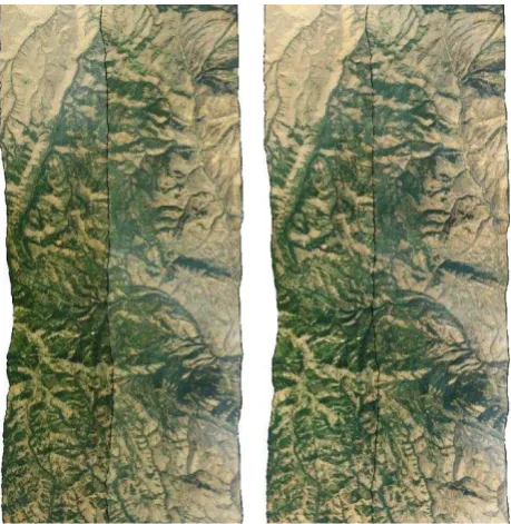
Figure 6 shows two overlapping image strips taken from an ortho-image mosaic in Idaho. The data has been captured using a Leica ADS100 sensor by North West Geomatics, Calgary, for the National Agriculture Imagery Program (NAIP); it is recti-fied to a GSD of 1.0 m. Especially in such mountain areas, the range of elevations causes differences in atmospheric impact that are not considered in the current ADS atmospheric model-ling. This leaves a considerable amount of localized haze after atmospheric and BRDF corrections and, therefore, nicely illus-trates the benefit – and also the need – of using radiometry fixes in the radiometric normalization over the initial, polynomial-based approach of Gehrke (2010).
Figure 6. Comparison of radiometric normalization approaches for a section of an ADS ortho-image overlap of approx. 100,000 pixels along strip. Left: Result from the polynomial correction model of Gehrke (2010); right: result from the new radiometry fix approach with a spacing of 5,000 pixels.
Band Input Images
Polyn. Model
R.F. 100,000
R.F. 20,000
R.F. 5,000
Red 151 103 106 101 97
Green 123 91 91 86 82
Blue 102 66 64 59 55
Table 1. Comparison of RMS DN differences at radiometric tie points before and after radiometric normalization adjustment with different approaches: polynomial model (Gehrke, 2010) vs. radiometry fix model with different along-strip spacing of 100,000, 20,000 and 5,000 image pixels between radiometry fixes.
The improvement of the strip-to-strip agreement is quantified by the RMS DN differences of radiometric tie points as shown in Table 1. Decreasing the radiometry fix spacing along strip provides more degrees of freedom and, accordingly, better adaptation. The RMS values after normalization are generally in the range of the initial standard deviation, i.e. about 10 % of the DN averages, which are in the order of 1,000 in this data set, depending on the band.
Resulting correction parameters are plotted along the center of the image overlap, exemplarily for the red image band, for con-trast in Figure 7 and for brightness in Figure 8. These plots generally confirm the need for a localized parameterization, even though for the smallest spacing of 5,000 pixels some of the resulting correction parameters become statistically insignifi-cant compared to their neighbours in the radiometry fix grid. To avoid confusion about the reduction of dynamic range as documented in Figure 7 (contrast < 1), it needs to be pointed out that – only for this investigation (!) – the average corrections of radiometry fixes are not constrained at image level (cp. section 3.4). This way they can be compared with the approach of Gehrke (2010) on a global scale – and readily illustrate local differences.
Figure 7. Contrast correction along an ADS strip (center of the overlap): ‘old’ polynomial model (Gehrke, 2010) vs. radiometry fix model with different along-strip spacing of 100,000, 20,000 and 5,000 image pixels between radiometry fixes.
Figure 8. Brightness correction along an ADS strip (center of the overlap): ‘old’ polynomial model (Gehrke, 2010) vs. radio -metry fix model with different along-strip spacing of 100,000, 20,000 and 5,000 image pixels between radiometry fixes.
Based on this type of investigation and the experience from processing large amounts of ADS data in day to day production work, a useful radiometry spacing of 20,000 pixels along strip has been found. Based on the ADS100 swath width of 20,000 pixels, the cells in the radiometry fix grid become square.
5.5 Large ADS Mosaic
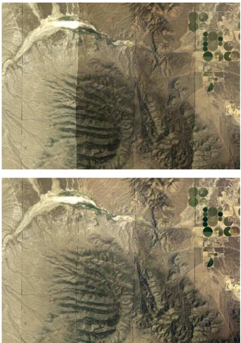
A typical ortho-image mosaic generated for, e.g., the Hexagon Imagery Program (HxIP; cp. Leica Geosystems, 2016) consists of input data from multiple sensors and flight sessions. An over-view of such a mosaic, located in Nevada, is shown in Figure 9. The data set has been captured and processed by North West Geomatics in 2015 using two ADS100 sensors. It consists of altogether 47 image strips from 8 flight sessions, which includes 5 images from 2 re-flight sessions. The final product is an ortho-image mosaic with 30 cm GSD.
Figure 9. ADS100 ortho-image mosaic in Nevada. Top: image strips after atmospheric and BRDF correction; bottom: result of the radiometric normalization. The rectangle marks the area of Figure 10.
Level Contrast Change Brightness Change RMS Min Max RMS Min Max
Session 0.12 -0.08 0.38 156 -340 250 Strip 0.05 -0.12 0.10 58 -165 147 R.F. 0.05 -0.23 0.15 28 -125 180 Overall 0.14 -0.38 0.47 168 -573 303
Table 2. Radiometric normalization parameters for the Nevada mosaic: RMS, minimum and maximum changes in contrast (factor) and brightness (DN offset) at different hierarchy levels (session, image strip and radiometry fixes within images).
Both the global comparison (Figure 9) and the local comparison (Figure 10) illustrate the in parts significant improvement by the radiometric normalization. A summary of correction parameters is provided in Table 2. The contributions at different hierarchy levels show that larger corrections at session level are required
for global mosaic adjustment, compensating the majority of differences as visible in Figure 10. The fact that the RMS cor-rections at the radiometry fixes are the lowest of all levels while their extrema are among the highest (cp. minimum contrast) underlines, again, the importance of sub-dividing images to model and apply localized corrections where required.
Figure 10. Sub-set of the ADS100 Nevada mosaic with the largest strip-to-strip differences before radiometric normali-zation. Top: imagery with atmospheric and BRDF corrections applied; bottom: final result after normalization.
6. SUMMARY AND OUTLOOK
We presented a new relative radiometric normalization, speci-fically targeted at large and, hence, radiometrically complex image mosaics. Key contributions are the localized correction model using radiometry fixes, the hierarchical modeling and the inherent preservation of (average) dynamic range. The benefit of all of which is illustrated for different examples from Leica Geosystems’ sensors.
The approach as implemented in HxMap software is generally robust and delivers successful results based on default settings for most practical applications. Nevertheless, the hierarchical parameterization allows for targeted adaptation. This is current-ly required for adjusting the oblique imagery from the Leica RCD sensors due to the largely varying view angles with very different atmospheric and ground reflectance properties. The current use of the presented approach includes the adjust-ment of imagery at different stages in the processing, namely at the time of ingesting a flight session and finally the generation of larger ortho-image mosaics. The normalization also benefits different kinds of other products, e.g., colorization of point
clouds – for which, again, different oblique views are still a challenge.
Also some of the examples in this paper – such as the water area – indicate that further research and refinements of the entire radiometric correction chain are needed to still improve results in certain conditions and applications.
REFERENCES
Al-Durgham, M., Downey, M., Gehrke, S., Beshah, B.T., 2016. A Framework for an Automatic Seamline Engine. Int. Arch. Photogramm. Rem. Sens., Prague, Czech Republic, Vol. XLI, Part B1 (this volume; submitted).
Baarda, W., 1968: A Testing Procedure for Use in Geodetic Networks. Publications on Geodesy, Netherlands Geodetic Commission, 5(2), pp. 1-97.
Beisl, U., Woodhouse, N., Lu, S., 2006. Radiometric Processing Scheme for Multispectral ADS40 Data for Mapping Purposes. Proc. ASPRS Annual Meeting, Reno, NV.
Beisl, U., Telaar, J., Schoenermark, M., 2008. Atmospheric Correction, Reflectance Calibration and BRDF Correction for ADS40 Image Data. Proc. Int. Arch. Photogramm. Rem. Sens.. Beijing, China, Vol. XXXVII, Part B1, pp. 7-12.
Chandelier, L., Martinoty, G., 2009. A Radiometric Aerial Triangulation for the Equalization of Digital Aerial Images and Orthoimages. Photogrammetric Engineering & Remote Sensing, 75(2), pp. 193–200.
Downey, M., Tempelmann, U., 2008. The “Photogrammetric Load Chain” for ADS Image Data – an Integral Approach to Image Correction and Rectification. Int. Arch. Photogramm. Rem. Sens.. Beijing, China, Vol. XXXVII, Part B2.
Downey, M., Uebbing, R., Gehrke, S., Beisl, U., 2010. Radio-metric Processing of ADS Imagery: Using Atmospheric and BRDF Corrections in Production. Proc. ASPRS Annual Confe-rence, San Diego, CA.
Falala, L, R. Gachet, and L. Chunin, 2008. Radiometric Block-Adjustment of Satellite Images – Reference3D Production Line Improvement. Int. Arch. Photogramm. Rem. Sens., Beijing, China, Vol. XXXVII, Part B4, pp. 319-324.
Gehrke, S., 2012. Combined Geometric/Radiometric Point Cloud Matching for Shear Analysis. Int. Arch. Photogramm. Rem. Sens., Melbourne, Australia, Vol. 39, Part B1.
Gehrke, S., Beshah, B.T., 2013. An Automated Approach for a Pluggable Multi-Sensor Triangulation. Proc. ASPRS Annual Conference, Balimore, MD.
González-Piqueras, J., Hernández, D., Felipe, B., Odi, M., Belmar, S., Villa, G., Domenech, E., 2010. Radiometric Aerial Triangulation Approach – A Case Study for the Z/I DMC. EuroCOW, Castelldefels, Spain.
Gruen, A., and L. Zhang, 2003. Sensor Modeling for Aerial Triangulation with Three-Line-Scanner (TLS) Imagery. Photo-grammetrie, Fernerkundung, Geoinformation, 2(2003), pp. 85-98.
Hinsken, L., S. Miller, U. Tempelmann, R. Uebbing, and S. Walker, 2002: Triangulation of LH Systems’ ADS40 Imagery Using ORIMA GPS/IMU. Int. Arch. Photogramm. Rem. Sens., Graz, Austria, 34(3A): 156-162.
Hong, G., 2007: Image Fusion, Image Registration, and Radio-metric Normalization for High Resolution Image Processing. University of New Brunswick, Technical Report No. 247.
Leica Geosystems, 2016: HxIP – Hexagon Imagery Program. http://www.leica-geosystems.us/en/HxIP-Hexagon-Imagery-Program_106454.htm (accessed: April 9, 2016).
Lopez, D.H., García, B.F., Piqueras, J.G., Alcázar, G.V., 2011: An Approach to the Radiometric Aerotriangulation of Photo-grammetric Images. ISPRS Journal of Photogrammetry and Remote Sensing, 66(2011), pp. 883-893.
McFeeters, S.K., 1996, The Use of Normalized Difference Water Index (NDWI) in the Delineation of Open Water Featu-res. International Journal of Remote Sensing, 17, pp. 1425-1432.
Molina, S., Villa, G., Serrano, C., Valdepérez, M., Domenech, E., 2010. A Polynomial Approach for Radiometric Aerial Trian-gulation. EuroCOW, Castelldefels, Spain.
Mulawa, D., 2000. Preparations for the On-Orbit Geometric Calibration of the OrbView 3 and 4 Satellites, Int. Arch. Photogram. Int. Arch. Photogramm. Rem. Sens., Amsterdam, Vol. XXXIII, Part B1, pp. 209-213.
Over, M., B. Schöttker, M. Braun, and G. Menz, 2003. Relative Radiometric Normalization of Multitemporal Landsat Data - A Comparison of Different Approaches. Proceedings IGARSS, Toulouse, France.
Pagnutti, M., Holekamp, K., Ryan, R.E., Sitton, D., 2015. Radiometric Corrections Workflow for Aerial Imaging Appli-cations. JACIE Workshop, Tampa, FL,
calval.cr.usgs.gov/wordpress/wp-content/uploads/ Pagnutti_JACIE2015RadiometricWorkFlow.pdf.
Pros, A., Colominaa, I., Navarroa, J.A., Antequerab, R., Andrinalb, P., 2013. Radiometric Block Adjustment and Digital Radiometric Model Generation. Int. Arch. Photogramm. Rem. Sens., Hannover, Germany, Vol. XL-1, Part W1.
Yang, X., and C.P. Lo, 2000: Relative Radiometric Normali-zation Performance for Change Detection from Multi-Date Satellite Images. Photogrammetric Engineering & Remote Sensing, 66(8), pp. 967-980.