ROAD ORTHOPHOTO/DTM GENERATION FROM MOBILE LASER SCANNING
Bruno Vallet, Jean-Pierre Papelard
IGN, Laboratoire MATIS 73 avenue de Paris 94165 Saint-Mand´e, FRANCE
[email protected] [email protected] recherche.ign.fr/labos/matis/∼vallet
Commission IIIWG III/3
KEY WORDS:Orthophotography, Digital Terrain Model, Road, Mobile laser scanning
ABSTRACT:
This paper proposes a pipeline to produce road orthophoto and DTM from Mobile Laser Scanning (MLS). For the ortho, modern laser scanners provide a reflectance information allowing for high quality grayscale images, at a much finer resolution than aerial photography can offer. For DTM, MLS offers a much higher accuracy and density than aerial products. This increased precision and resolution leverages new applications for both ortho and DEM. The first task is to filter ground vs non ground, then an interpolation is conducted to build image tiles from the filtered points. Finally, multiple layers are registered and blended to allow for seamless fusion. Our proposed approach achieves high quality products and scaling up is demonstrated.
1. INTRODUCTION
1.1 CONTEXT
Orthophotography and Digital Terrain Models (DTM) are ubiq-uitous and very standard products in the aerial photogrammetry pipeline. Their applications are numerous in remote sensing, ge-ographical information and earth observation sciences, mapping, urban planning,... These products are traditionally built from satellite and aerial imagery, with a recent trend towards UAVS to increase resolution at the cost of lower productivity. However, to study urban cores in fine details, these products are limited by their resolution, accuracy, and occlusions (mainly by trees and tall buildings). In this paper, we advocate that ortho and DTM can be built from Mobile Laser Scanning (MLS) to overcome some of these limitations. The possible applications of such products are:
• Precise mapping of road marks (Hervieu et al., 2015), road limits (McElhinney et al., 2010) or curbs (El-Halawany et al., 2011) (Zhao and Yuan, 2012) (Hervieu and Soheilian, 2013b),...
• Road inventory (Pu et al., 2011)
• Road surface modelling (Hervieu and Soheilian, 2013a) and quality analysis
• Itinerary computations and public building accessibility for soft mobilities (disabled, strollers, ...) (Serna and Marcotegui, 2013)
• Mobile mapping registration on aerial images (Tournaire et al., 2006)
• Image based localization using ground landmarks (Qu et al., 2015)
• Water flow simulations
In some European countries in particular, recent legislation calls for a subdecimetric accuracy mapping of buried objects (water and gas pipes, wires, ...) because the lack of precise data cause ac-cidents and delays in many public construction works. This map-ping calls for a precise occlusion free orthophoto of the ground surface.
1.2 RELATED WORKS
To our knowledge, the problem of generating an orthophoto from the intensity of a laser scan has scarsely been investigated, but it is mainly a problem of dense interpolation from sparse points that we will discuss in this Section. On the other hand, the problem of extracting a DTM from laser scanning is widely studied, the main challenges being the registration of overlapping strips, the filter-ing of ground vs off ground points, and the interpolation required to produce a dense image from sparse unstructured points.
Registration of MLS is usually based on ICP which alternates making matches and finding the transformation that minimizes distance between these. They can be separated depending on the sought transformation: either the data is split into rectilin-ear blocks that are rigidly registered (Gressin et al., 2012a), or a a non rigid transformation is sought for, the popular choice be-ing a translation linearly interpolated in time (Takai et al., 2013) (Monnier et al., 2013). The matches used for this registration are point-to-point or point-to-plane (or both), and matches are fil-tered based on a distance criterion that can be enhanced using local feature (Gressin et al., 2012b).
Projection
Registration Registered DTM Blending ortho/DTMBlended Laser
scans
Figure 1: Full ortho/DTM production pipeline from MLS. Framed rectangles are processing steps, unframed rectangles are exchanged data types. The pipeline input/output is in yellow.
Laser Scanning (MLS), this extraction can be done based on ele-vation and gradient features (Zhao and Yuan, 2012), based on ex-tracting large planes at a certain distance below the 3D trajectory of the laser scanner and analysing them (Pu et al., 2011) or with Robust Locally Weighted Regression (Nurunnabi et al., 2013).
Concerning the interpolation problem, the most popular approach in ALS is Kriging (Kraus and Pfeifer, 2001) as it has a strong statistical support, but other popular approaches such as Moving Least Squares and Inverse Distance Weighting (Shan and Toth, 2008) are often used for their simplicity. If the desired output is a Triangular Irregular Network (TIN), then a Delaunay Triangula-tion should be performed instead of interpolaTriangula-tion (Xiaobo et al., 1999). For MLS, (Bitenc et al., 2011) propose a linear interpola-tion based on plane fitting with the purpose of error propagainterpola-tion, but this is only suited to their sandy coast monitoring application where the pixel size if very large (1m) compared to ours (4cm). In this paper, we chose a Poisson interpolation (P´erez et al., 2003) as our pixel size is very small and sampling density is very variable, with large holes from occlusions that need to be filled.
1.3 METHOD OVERVIEW
A major issue in producing a DTM is the filtering of on ground vs off ground points which will be done based on both a global height estimation and local planarity priors. This will be dis-cussed in Section 2.. Then a Poisson interpolation method used for both ortho and DTM will be presented in Section 3.. The non-rigid altimetric registration problem will be tackled in Section 4.. Then the tiles blending for multiple passages will be described in Section 5.. Results will be presented and discussed at each step of the pipeline (Sections 2. to 5.). Finally conclusions will be drawn in Section 6.. The full pipeline is illustrated in Figure 1.
1.4 DATA PRESENTATION
The data used in this study is a Mobile Laser Scan (MLS) ac-quired by the mobile mapping system described in (own citation). The scan was performed in around 3 hours in a very dense ur-ban environment, covering around 15 linear kilometres of city streets. The sensor is a RIEGL LMS-Q120i that was mounted transversally in order to scan a plane orthogonal to the trajectory. It rotates at 100 Hz and emits 3000 pulses per rotation, which corresponds to an angular resolution around0.12◦
. Each pulse can result in 0 to 8 echoes producing an average of 250 thousand points per second. The resulting scan is very anisotropic because
Figure 2: A view of the Mobile Laser Scan (MLS) used in this study, coloured with reflectance.
while points are very dense along scanlines (a few mm on the road below the sensor), scanlines can be separated by several cms ac-cording to the vehicle speed (5cm at a typical acquisition speed of 5m/s = 18km/h). In addition to the(x, y, z)coordinates (in sensor space), the sensor records multiple information for each pulse (direction, time of emission) and echo (amplitude, range). The amplitude being dependant on the range, it is corrected into a relative reflectance. This is the ratio of the received power to the power that would be received from a white diffuse target at the same distance expressed in dB. The reflectance represents a range independent property of the target.
The Stereopolis mobile mapping system is also composed of an Applanix POS-LV220 georeferencing system combining D-GPS, an inertial unit and an odometer. However, the GPS masks that frequently occur in urban areas induce drifts that can reach one meter for a 2 minutes mask. This initial georeferencing is cor-rected based on tie points with aerial photography resulting in around 10cm standard deviation in planimetry, and 15cm in al-timetry.
The laser sensor is calibrated in order to recover the transforma-tion between the sensor and Applanix coordinate systems which allows to transform the(x, y, z)coordinates from sensor to a ge-ographic coordinate system. The result, with a colormap on re-flectance, is displayed in Figure 2.
2. GROUND FILTERING
In order to produce a Digital Terrain Model (DTM), the off-ground points need to be filtered off. This filtering can be performed ei-ther directly on the points cloud or in the image space in which we wish to represent our DTM. We chose an image based filtering for efficiency, so we first need to discuss how we produce images from our MLS.
2.1 TILES AND LAYERS
Our input for DTM/Orthophoto generation is a mobile mapping point cloud, which has several specificities:
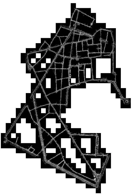
Figure 3: Mobile laser scan reflectance projected into the 412 tiles of our area of study. A single tile is shown on Figure 4 (top)
• The overlaps are very specific: they happen either at road in-tersections, or along road sections that the vehicle has cov-ered more than once (which often happens as it is not avoid-able when an extensive coverage of the roads is required).
As our aim is to generate raster based products (DTM and Or-thophoto), we need to tile the area of study in a way that takes these specificities into account. First, we use 50m by 50m tiles which size is the order of the efficient range of the laser scan. This is a good compromise between the number of tiles and the unused area (area covered by a tile but not by the scan). Con-cerning the pixel resolution, we chose a 4cm pixel (1250 x 1250 px tiles) which is below our expected absolute accuracy (10cm), and a good compromise between storage requirement and accu-racy. It is not easy to adapt the pixel size to the scan horizontal density as it is very variable according to the scene geometry and distance from sensor. It is also very anisotropic because points are very dense along scanlines (a few mm on the road below the sensor), but scanlines can be separated by several cms according to the vehicle speed (5cm at a typical acquisition speed of 5m/s = 18km/h). That latter consideration also advocates for a pixel size around 4cm (close to the distance between scanlines). A view of this tiling over the whole area of study is given in Figure 3.
As we need to convert to image space at one point of our pipeline anyways, we would like to do it as soon as possible such all the processing is done with image tools, which are generally faster that point cloud processing tools (in particular thanks to trivial neighbourhoods). So the first step of the DTM/Ortho production pipeline could be to project all the points from the laser scan in such tiles. However, we prefer to keep the various passages
sepa-rated in order to allow for a fine altimetric registration (cf Section 4.), that is to generate not one image for each tile, but as many as the number of times that the MMS has acquired points over that tile. This is done based on time: points are projected in the or-der that they were acquired, and an active layer is created when a point projects on a tile where there is no active layer. After a cer-tain time without points projecting in it, an active layer become inactive (and is stored to the disk as a complete layer). This way, if the acquisition comes back to the same tile, a new layer will be created. This process produces frequently 2 to 3 layers on some tiles, and up to 5 in our experiments. On our area of study, this process generated 1022 layers (1.6.109pixels) on 412 tiles.
Finally, we need to detail how we convert the point cloud in a raster during the accumulation. For each pixel, if no point projects in it we store a ”no-data” information defining adata maskMdata. If one point or more projects in a pixel, we keep the lowest onePlow (because our aim is to model the ground) and store in the pixel:
• Thezcomponent ofPlow
• The range ofPlow(distance betweenPlowand the laser cen-ter)
• The relative reflectance of the target atPlow. • The acquisition time ofPlow
all of which will be used in latter steps. An illustration of this ras-terization for the relative reflectance image is displayed in Figure 4(a). After this rasterization step, all the subsequent steps detailed in this paper are performed in image space (2.5D for DTM, 2D for the other features).
2.2 GROUND FILTERING
Now that the points are projected in independent layers, the main remaining issue is to define what is a ground point and what isn’t. A simple definition for the ground in urban areas is that it con-sists of points which lie on a locally planar and horizontal surface patch. However this definition does not tackle points on flat roof surfaces, so we also need either a building detection, or more simply a good local approximation of where the ground is. For a mobile laser scan (MLS), there is a simple such approximation that we describe in Section 2.2.1. For the horizontal planarity, we propose a simple filter in Section 2.2.2.
2.2.1 ELEVATION FILTERING With MLS, we have an easy tip on where is the ground: the vehicle acquiring the point cloud is lying on it (more precisely on the road surface). Knowing the heighthsensorof the laser sensor referentialRsensor above the ground, and the 3D points coordinates inRsensor, we can simply filter out points according to their vertical component inRsensor, by keeping points satisfying:
zsensor∈[hsensor−δ1, hsensor+δ1] (1)
where the parameterδneeds to be chosen according to the speci-ficities of the studied area, and in particular the type of locally planar horizontal surfaces that might exists close to the ground.
furniture, ...) that might still have a part in the previously se-lected points. To filter out these points, we use the strong prior that the ground is locally a plane close to horizontal by analysing two vertical cylindrical neighbourhoods with the same radiusrcyl for each pointP. The first cylinderC∞is infinite inzwhile the second cylinderCδ2 is limited to[Pz−δ2, Pz+δ2]. If a suf-ficient proportion of points inC∞are also in Cδ2, this means thatP belongs to a sufficiently horizontal planar surface so we keep it, else we remove it. Note that this filtering is computed from thezcomponent of each layer, but also applied to the other component such that their interpolation will only be performed on ground points.
2.3 RESULTS
The ground points filtering described here gives very satisfactory results as the local filter achieves to remove most points on ob-jects lying on the ground to keep only points on the ground itself. Concerning timings, this filtering is very fast to compute. It took a few minutes on our 1022 layers in single thread on an Intel Core i7 CPU at 3.33GHz.
3. POISSON INTERPOLATION
A DTM is a raster representation of a surface without overhangs. The filtered point cloud from the previous section is sparse, in the sense that it does not cover all the pixels of the DTM, which calls for an interpolation of the height component. However, with mo-bile mapping, one cannot hope for an integral coverage of some area (defined by a bounding box for instance), but only of a lim-ited strip along the trajectory of the mobile mapping system that acquired the data, which precise footprint depends on the scene and acquisition geometries. In order to interpolate between the points, the first question we have to answer is thus where do we want to interpolate ? We will answer explicitly to this question by creating a mask defining where we want to interpolate tion 3.1), then explain how the interpolation is performed (Sec-tion 3.2).
3.1 INTERPOLATION MASK DEFINITION
Interpolation allows to fill holes and gaps in the data. The mask should be adapted to the application of the DTM. In our case, the targeted application was producing slope maps to assess the accessibility of public buildings to wheelchairs. Thus we need to smoothly interpolate the DTM everywhere on the side-walk, and in particular in its occlusion by cars, pedestrians,... On the other hand, we also want to remove isolated points that are useless for that purpose. This is why we chose to apply a succession of morphological dilation/erosions:
• A dilation of 10px (40cm) to connect neighbouring points. • A closure (erosion then dilation) of 30px (1.2m) to remove
isolated points. Because of the previous dilation, it removes isolated point groups of size around 80cm.
• A dilation of 90px (3.6m) to fill occlusions by objects of the size of a car.
The result is called theinterpolation maskMinter. Its bound-ary is very smooth and it extends 4m around the areas where the points density is sufficient (less than 40cms between two points). Optionnaly, if a database of the buildings’ footprints is available on the area of study (such as a cadaster), it can be integrated in this mask to avoid extrapolating the ground inside the buildings.
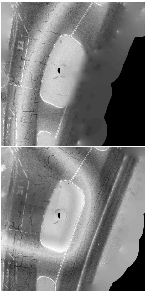
(a) MLS layer in a tile (f)
(b) Poisson interpolationu∗offinside a mask
Figure 4: Illustration of Poisson interpolation on the reflectance component
3.2 INTERPOLATION
Poisson interpolation expresses simply the interpolation problem as that of finding a functionuthat approximates a functionfas closely as possible wherefis defined and is as smooth as possible where is is not, which is exactly the behaviour that we want for DTM generation. In our case, this is done by minimizing:
EP oisson=X Sf
|u−f|2+λ X
(i,j)∈N4(Minter)
∇u (2)
whereSf is the support of f (pixels where at least one point projects) and:
N4(Minter) ={(i, j)|i∈Minter, j∈Minter
andi, jare 4-connected}
is the set of (4-connected) neighbours inMinter (computed in Section 3.1).
The solution to (2) is obtained by putting it in matrix form:
where:
• fis the (known) vector of data pixel values of sizendata • uis the (unknown) vector of interpolated pixel values of size
ninter
• Adatais the(ndata, ninter)matrix of valueai,j = 1ifui andfj correspond to the same pixel (else 0). It is created from the chosen indexation for pixels from the data and in-terpolation masks.
• Gis the(ndata, nneigh)is the gradient matrix of termgi,(i,j)
= 1,gj,(i,j)=−1for all neighbours(i, j)∈N4(Minter)
The minimizer of (3) is given by:
u∗= (AtA+λGtG)−1Atf (4)
In practice, we used theLDLtfactorization from the Open source library Eigen, which takes around 20s per tile. Once computed, (4) can be calculated very efficiently for all dataf that we want to interpolate (z, reflectance, range, time).
3.3 RESULTS
The data involved in interpolation (MLS projection in a tile, mask and Poisson interpolation in the mask) is shown in figure 4, where the reflectance is used to illustratef (top) andu(bottom). The interpolation result for the other layers of the same tile are shown in Figure 5. Note that the same interpolation process is also ap-plied to thez, range and time components (not shown here but used in the next Sections).
This step of the pipeline is the most time consuming because of the factorization. It is however very easy to parallelize as the computation is independent on every tile. The whole interpola-tion process (including mask generainterpola-tion and interpolainterpola-tion ofz, reflectance, time and range) took around 2 hours on 10 threads an Intel Core i7 CPU at 3.33GHz.
A drawback however of the tiling is that we do not ensure conti-nuity across tiles. This is however minor because the interpola-tion is based on the MLS, so if the MLS is continuous across the tile boundary, so will its interpolation. However, if an occlusion running across a tile boundary needs to be filled, continuity will not be ensured. For our application, we used the DTM to com-pute slopes (gradient) which is also tile based, so a discontinuity across boundary will not generate a high slope. If discontinuities are a problem for the desired application, then borders should be added to the tiles in order to enable a seamless blending.
4. NON RIGID ALTIMETRIC REGISTRATION
As explained in Section 2.1, we chose to split the tiles in layers according to the passages of the vehicle in order to allow for a fine registration. As explained in Section 1.4, the vertical abolute accuracy of our MLS is around 15cm. For our building accessi-bility application, 15 cm is not sufficient as blending tiles might induce a false 15cm step that cannot be climbed by a wheelchair resulting in an erroneous decision. This is why we propose a non rigid registration procedure inspired by (Monnier et al., 2013).
Figure 5: Illustration of Poisson interpolation on the other two layers of the tile of Figure 4
4.1 NON RIGID DEFORMATION MODEL
We propose an adaptation and simplification of (Monnier et al., 2013) in order to register the layers inZonly (which is our main issue for DTM generation). The method relies on the definition of a non-rigid deformation defined by a translation given atnT control timesTcand linearly interpolated in between. The first difference is we only look for a translation in thezdirection, so our unknowns are simplynTshifts inz:δcz.
4.2 ICP BASED REGISTRATION
The registration is then done following the principle of ICP:
1. Match points between layers
2. Find the deformation that minimizes distance between matched points
For the matching, the tile structures makes it obvious: for each tile, we match pixels from each pair of layers in their intersec-tion. For robustness, we keep only the matches for which the difference inz is below the mean absolute difference over the tile intersection. This avoids the necessity to choose a threshold and decide how it will decrease and naturally adapts to all inputs. Thus a matchmis characterized by the tile it belongs to, the two layersiandjinvolved in the tile, the pixelpon which it occurs and the valueszi(p),zj(p)andti(p),tj(p)of the DTM and time from the two layers on that pixelp, resulting from the interpola-tion of Secinterpola-tion 3.. Once the matches are selected, we minimize:
EICP(δz1,· · ·, δ
z nT) =
X
matches
||zi+δz(ti)−zj−δz(tj)||2
+γ nXT−1
i=1
(δiz−δ z
i+1)2 (5)
whereδzis the linear interpolation of the translation inz:
δz(t) =α(t)δzc+(t)+(1−α(t))δzc−(t) α(t) =
t−Tc−(t)
Tc+(t)−Tc−(t)
andc−
(t)andc+(t)are the indices of the control times before and aftert.γis a rigidity parameter reflecting the confidence we have in the shape of the trajectory given by the georeferencing system. Equation (5) can be written in matrix form:
EICP(z) =||Mz+ ∆z||2+γ||Dz||2 (6) where:
• zis the vector of shifts inz δiz
• Mis the (nT,nmatch) matches matrix which non null terms are:
Mc+(t
i),m=α(ti) Mc−(ti),m= 1−α(ti)
Mc+(t
j),m=−α(tj) Mc−(tj),m=α(tj)−1
for each matchm.
• ∆z
is the vector of termzi−zjfor each match.
The minimum of Equation (6) is given by:
z∗
=−(MtM+γDtD)−1
Mt∆z (7)
Finally, for the stopping criterion, we simply chose a 1mm thresh-old on the average|δz
i|which is more than sufficient for our pur-pose and is usually reached in less than 5 iterations.
4.3 RESULTS
In our experiments, we take one control time every second for a 3 hours acquisition such thatnT ≈104. Computing (7) requires
inverting a sparse symmetric matrix of sizenT, which takes much less than a second using the Open source library Eigen. The most time consuming step is in fact the matching because we need two passes for each layer (one to compute the average and one to compute the matches), which can be optimized by subsampling, yielding a total computation time for the registration of 10 min-utes (for one ICP iteration) for the 1022 layers in single thread on an Intel Core i7 CPU at 3.33GHz.
A close-up on slices of two DTM layer is shown before and after registration on Figure 6. On this example, the registration reduces
Figure 6: Registration result for two DTM layers (one textured and one in white wireframe). Top: before registration. Bottom: after registration. The scale is given by the step of the wireframe (4cm)
the shift in Z from 30cm to below 2cm. In average, over the whole 20kms of the acquisition, our non-rigid registration lowers the average shift in Z from 16cm to 4.3cm in the first iteration and 3.7cm in the second and ends at 3.5cm at iteration 4, for a total computation time of 40 minutes.
5. TILES BLENDING
5.1 EXPONENTIAL BLENDING
Once the layers are registered, they can be blended in order to produce the final tiles. That blending needs to be adapted to the specific geometry of a MLS. In particular, we want smooth tran-sitions between layers, and we want to give more weight to the points which are the closest to the sensor (because the resolution, precision and reflectance information are better for points closer to the sensor). To fulfil these requirements, we found that a good choice was an exponential weighting in the range, which is why we interpolate it in Section 3.:
W(p) = exp(−φ.range(p))
areas look less sharp. In practice, we choseφ= 1mensuring a good compromise between transition smoothness and sharpness.
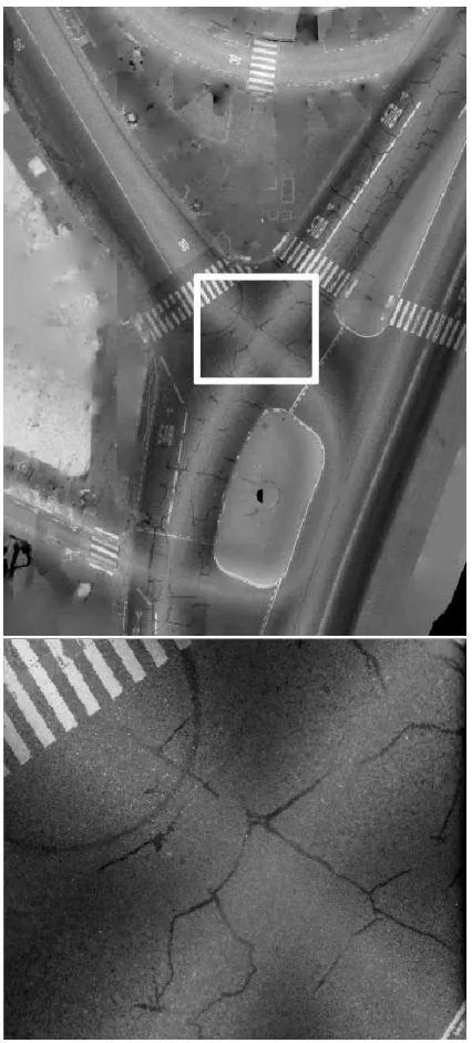
Figure 7: Blending result for reflectance image on an area around the tile which layers are displayed in Figures 4(b) and 5 and a close up near a trajectory crossing.
5.2 RESULTS
A results of this blending procedure for reflectance is given on Figure 7. We see the vehicle trajectories as highlights on the ground because the road has a specular component that makes the backscattered intensity higher for near orthogonal incidence angles. Despite multiple crossing or overlapping trajectories in the same area, the blending achieves a smooth result without vis-ible seams or blending artefacts. This result has a much better quality than an aerial orthophoto and ability to see under the veg-etation as illustrated in Figure 8. The laser sensor used emits in near red, so the resulting orthoimage can be seen as an infra-red image that is very independent of the lighting conditions (no shadow) because the sensor is active. Another possible output of this pipeline is a DTM surface textured with the reflectance or-tho as shown in Figure 9. Because both information come from
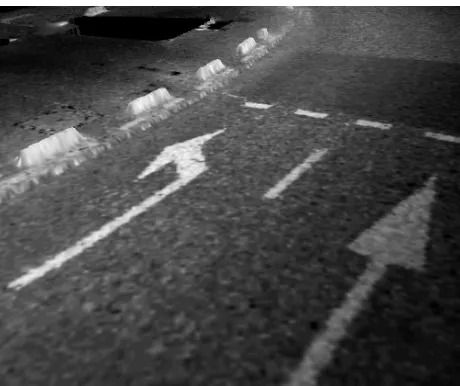
Figure 8: Comparison of a 20cm aerial orthophoto (top) with a MLS orthophoto (bottom).
the same data (the MLS) geometry and radiometry are perfectly aligned, resulting in a high quality textured ground model.
Blending with this procedure is extremely fast and took below one minute to generate 412 final tiles (DTM and ortho) from the 1022 layers in single thread on an Intel Core i7 CPU at 3.33GHz. Overall, the whole Ortho/DTM generation took around 3 hours for a 3 hours acquisition, which shows that they can be produced as fast as the data is acquired on a single laptop which is very promising for a possible industrialization.
6. CONCLUSIONS AND FUTURE WORK
The DTM produced by our pipeline has been successfully inte-grated in a GIS that exploited this information to assess accessi-bility of public buildings to the disabled and provide an itinerary computation service for soft mobilities (wheelchairs, strollers,...) The reflectance image was used for visualization only in this sce-nario. However, we believe that this highly accurate DTM/ortho from MLS can be used in a variety of other applications such as precise image based localization, road surface quality assessment and defaults detection, water flow simulations, road surface mod-elling, curb detection and road marks extraction.
Figure 9: Digital Terrain Model textured with the reflectance or-thophoto
poles, ...) would appear with color codes to distinguish them, and with transparency to handle multiple layers. The result would be an orthophoto where all the scanned elements would appear even if not visible from above.
ACKNOWLEDGEMENTS
This work has been performed as part of the Cap Digital Business Cluster TerraMobilita Project.
REFERENCES
Bitenc, M., Lindenbergh, R., Khoshelham, K. and Van Waarden, A. P., 2011. Evaluation of a lidar land-based mobile mapping sys-tem for monitoring sandy coasts. Remote Sensing 3(7), pp. 1472– 1491.
El-Halawany, S., Moussa, A., Lichti, D. D. and El-Sheimy, N., 2011. Detection of road curb from mobile terrestrial laser scan-ner point cloud. In: International Archives of Photogrammetry Remote Sensing and Spatial Information Sciences, Vol. 2931, pp. 29–31.
Gressin, A., Cannelle, B., Mallet, C. and Papelard, J.-P., 2012a. Trajectory-based registration of 3d lidar point clouds acquired with a mobile mapping systems. In: ISPRS Annals of Pho-togrammetry, Remote Sensing and the Spatial Information Sci-ences, Melbourne, Australia, August, Vol. 1-3, pp. 117–122.
Gressin, A., Mallet, C. and David, N., 2012b. Improving 3d lidar point cloud registration using optimal neighborhood knowledge. In: ISPRS Annals of Photogrammetry, Remote Sensing and the Spatial Information Sciences, Melbourne, Australia, August, Vol. 1-3, pp. 111–116.
Hervieu, A. and Soheilian, B., 2013a. Road side detection and reconstruction using lidar sensor. In: IEEE Intelligent Vehicles Symposium (IV), pp. 1247–1252.
Hervieu, A. and Soheilian, B., 2013b. Semi-automatic road/pavement modeling using mobile laser scanning. In: IS-PRS Annals of Photogrammetry, Remote Sensing and the Spatial Information Sciences, Vol. II-3/W3, pp. 31–36.
Hervieu, A., Soheilian, B. and Br´edif, M., 2015. Road marking extraction using a model and data-driven rj-mcmc. In: ISPRS Annals of Photogrammetry, Remote Sensing and the Spatial In-formation Sciences, Vol. 1, pp. 47–54.
Kraus, K. and Pfeifer, N., 2001. Advanced dtm generation from lidar data. International Archives Of Photogrammetry Remote Sensing And Spatial Information Sciences 34(3/W4), pp. 23–30.
McElhinney, C., Kumar, P., Cahalane, C. and McCarthy, T., 2010. Initial results from european road safety inspection (eursi) mobile mapping project. International Archives of the Photogramme-try, Remote Sensing and Spatial Information Sciences 38, Issue PART 5, pp. 440–445.
Monnier, F., Vallet, B., Paparoditis, N., Papelard, J.-P. and David, N., 2013. Registration of terrestrial mobile laser data on 2d and 3d geographic database by use of a non-rigide icp approach. In: ISPRS Annals of Photogrammetry, Remote Sensing and Spatial Information Sciences, Vol. II-5/W2, pp. 193–198.
Nurunnabi, A., West, G. and Belton, D., 2013. Robust locally weighted regression for ground surface extraction in mobile laser scanning 3d data. In: ISPRS Annals of Photogrammetry, Remote Sensing and Spatial Information Sciences, Vol. 1.2, pp. 217–222.
P´erez, P., Gangnet, M. and Blake, A., 2003. Poisson image edit-ing. In: ACM Transactions on Graphics (TOG), Vol. 22number 3, ACM, pp. 313–318.
Pu, S., Rutzinger, M., Vosselman, G. and Elberink, S. O., 2011. Recognizing basic structures from mobile laser scanning data for road inventory studies. ISPRS Journal of Photogrammetry and Remote Sensing 66(6, Supplement), pp. S28 – S39. Advances in LIDAR Data Processing and Applications.
Qu, X., Soheilian, B. and Paparoditis, N., 2015. Vehicle local-ization using mono-camera and geo-referenced traffic signs. In: IEEE Intelligent Vehicles Symposium (IV), pp. 605–610.
Rottensteiner, F. and Briese, C., 2002. A new method for building extraction in urban areas from high-resolution lidar data. Interna-tional Archives of Photogrammetry Remote Sensing and Spatial Information Sciences 34(3/A), pp. 295–301.
Serna, A. and Marcotegui, B., 2013. Urban accessibility diag-nosis from mobile laser scanning data. ISPRS Journal of Pho-togrammetry and Remote Sensing 84(0), pp. 23–32.
Shan, J. and Toth, C. K., 2008. Topographic laser ranging and scanning: principles and processing. CRC Press.
Takai, S., Date, H., Kanai, S., Niina, Y., Oda, K. and Ikeda, T., 2013. Accurate registration of mms point clouds of urban areas using trajectory. In: ISPRS Annals of Photogrammetry, Remote Sensing and Spatial Information Sciences, Vol. 1.2, pp. 277–282.
Tournaire, O., Soheilian, B. and Paparoditis, N., 2006. Towards a sub-decimeter georeferencing of ground-based mobile mapping systems in urban areas : Matching ground-based and aerial-based imagery using roadmarks. In: International Archives of Pho-togrammetry, Remote Sensing and Spatial Information Sciences., Vol. 36 (Part 1).
Wack, R. and Wimmer, A., 2002. Digital terrain models from airborne laserscanner data-a grid based approach. International Archives of Photogrammetry Remote Sensing and Spatial Infor-mation Sciences 34(3/B), pp. 293–296.
Xiaobo, W., Shixing, W. and Chunsheng, X., 1999. A new study of delaunay triangulation creation [j]. ACTA Geodaetica et Car-tographic Sinica.