PROJECTIVE TEXTURING UNCERTAIN GEOMETRY: SILHOUETTE-AWARE
BOX-FILTERED BLENDING USING INTEGRAL RADIAL IMAGES
Mathieu Br´edif
Universit´e Paris-Est, IGN, SRIG, MATIS, 73 avenue de Paris, 94160 Saint Mand´e, France mathieu . bredif @ ign . fr
KEY WORDS:Projective texturing, Uncertainty, Image based rendering
ABSTRACT:
Projective texturing is a commonly used image based rendering technique that enables the synthesis of novel views from the blended reprojection of nearby views on a coarse geometry proxy approximating the scene. When scene geometry is inexact, aliasing artefacts occur. This introduces disturbing artefacts in applications such as street-level immersive navigation in mobile mapping imagery, since a pixel-accurate modelling of the scene geometry and all its details is most of the time out of question. The filtered blending approach applies the necessary 1D low-pass filtering on the projective texture to trade out the aliasing artefacts at the cost of some radial blurring. This paper proposes extensions of the filtered blending approach. Firstly, we introduce Integral Radial Images that enable constant time radial box filtering and show how they can be used to apply box-filtered blending in constant time independently of the amount of depth uncertainty. Secondly, we show a very efficient application of filtered blending where the scene geometry is only given by a loose depth interval prior rather than an actual geometry proxy. Thirdly, we propose a silhouette-aware extension of the box-filtered blending that not only account for uncertain depth along the viewing ray but also for uncertain silhouettes that have to be blurred as well.
1 INTRODUCTION
1.1 Context
Many 3D visualization applications do not really require a pre-cise and accurate modelling of the scene geometry and radiome-try. What is really required in the end is the synthesis of a novel viewpoint with minimal temporal or spatial artefacts and the best quality possible. By bypassing the modelling step, that is what image-based rendering techniques are targeting (Br´edif, 2013).
1.2 Rendering uncertain geometry
The geometry of the real world is only captured (stereo recon-struction, lidar sensing...) at a given resolution, up to a certain level of accuracy and with some amount of noise and outliers. We are interested in propagating this uncertainty of the geometry (point cloud, 3D model...) to the rendering to prevent arbitrary decision and information loss.
Hofsetz (2003) proposed an image based rendering technique that handles a point cloud with uncertainty. Each point is splat on the screen using its uncertainty ellipse to get the relevant filter-ing. This approach gives satisfactory results but scales not so well with the number of uncertain points.
The filtered-blending approach of Eisemann et al. (2007) is mo-tivated by the fact that an incorrect geometric approximation of the scene will yield aliasing artefacts when colored by projecting multiple textures on it. They proved that only a 1D filtering was needed to prevent that aliasing. A second approach is to let the projective parameters of the texture evolve so as to reduce the vis-ible artefacts. This is the floating texture approach of Eisemann et al. (2008).
The Ambient Point Cloud method (Goesele et al., 2010) has been developed in the context of multi view stereo where part of the scene is densely reconstructed, part of the scene is composed of a sparse point set and some pixels do not have any depth esti-mate, each with a different rendering mode in accordance to the different nature of geometric uncertainty. This paper introduced
a notion similar to Eisemann et al. (2007) that uncertain depth may be rendered as a linear filtering in the epipolar motion di-rection. They however preferred a filtering based of sparse and jittered point samples rather than the low-pass filtering discussed in Eisemann et al. (2007).
1.3 Contributions
Focusing on box filters, we propose to extend the filtered-blending approach of Eisemann et al. (2007) in a number of aspects :
• We adapt the concept of constant time box filtering provided by 2D-integral images to computing box-filtered blending with a performance which is independent of the blur ex-tent, by introducing the integral radial images (sections 2 and 3.2).
• Application-wise, we show how this method may be straight-forwardly adapted to projective-textured scenes where ge-ometry is given only by a loose depth prior, which yields satisfactory results in the showcased street-level navigation context (section 3.1).
• Lastly, our main contribution is an extension of box-filtered blending that handles uncertain silhouette boundaries (sec-tion 3.3).
2 CONSTANT-TIME BOX-FILTERED BLENDING
2.1 Epipolar Filtering
Interpolated View
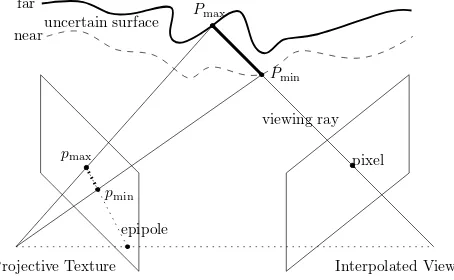
Figure 1: Epipolar filtering geometry
For a given pixel, scene uncertainty translates into an uncertainty of the 3D location (e.g. [Pmin, Pmax]in figure 1) of the inter-section of the 3D pixel ray with the scene, and consequently to an uncertain 2D position on the corresponding epipolar ray (e.g.
[pmin, pmax]in figure 1). The kernel used in filtered blending is essentially defining, for each projective texture to be blended, a probability density of this 2D location on the epipolar ray in ordered to compute its expected value.
As all pixel rays will reproject to epipolar rays, the resulting ex-pected values will all be integrated over linear supports that meet at the projective texture epipole. Thus, the filters used in the fil-tered blending of each projective texture reduce to 1D filters in a radial setup with a pole fixed at the epipole.
The most simple probability density is a uniform density over the subset of the 2D epipolar rays that correspond to the projection of plausible view ray / scene intersections. This uniform density translates into radial 1D-box filters around the epipole.
2.2 Linear-Time Filtered Blending
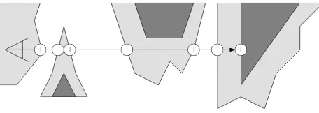
With box filtering, filtered blending requires computing average pixel values over line segments. For segments of small length, the marching along this line segment may be performed exhaustively by stepping through and sampling directly the original texture. However, for longer segments, the linear increase of samples (texture lookups) becomes a performance bottleneck. A quick and dirty solution is to limit the number of samples along the segment to a fixed maximum. This may be approximated and implemented in a number of ways including (figure 2) :
• No prefiltering. This generates, for long segments, a grainy look similar to what is achieved in the Ambient Point Cloud approach (Goesele et al., 2010), which may lead to aliasing or temporal incoherence due to the unfiltered point sampling of the input texture.
• Isotropic prefiltering. This approach aims to approximate the integral over the linear segment as a sum of samples on a blurred (i.e. band-limited) image. It may be easily imple-mented using mipmap level biasing in the graphics pipeline. This however introduces a trade off between the necessary unaliasing blur along the segment and the unnecessary blur across the segment.
• Anisotropic prefilteringis available on the graphics pipeline for anisotropic sampling in arbitrary directions, addressing the issue of unwanted blurring across the segment direction. This approach is appealing but has the following downsides: 1) the amount of anisotropy is hardware-limited, yielding
Anisotropic Isotropic None
Figure 2: Prefiltering options for subsampling 1D integrals
only a linear reduction on the number of texture samples, as in the previous two options. 2) The combination of the hardware-provided anisotropic filter kernels only provide an approximation of the desired linear integral.
These approaches do not feature the same factor but all have nonetheless a linear time-complexity relative to the length of the projected segment. By restricting ourselves to linear box filtering, we demonstrate how the epipolar nature of the filtering geometry (section 2.1) may be used to implement box-filtered blending in constant-time (section 2.3).
2.3 Constant-Time Box-Filtered Blending with Integral Ra-dial Images
We introduce the integral radial image at a given pole as a pre-pocessed image that enables the computation of 1D box filters in constant time, provided that the supporting line of the box filter passes through the pole of the integral radial image. The compu-tation of the integral radial image of a image at a given pole is performed as follows:
1. Resample the image in radial geometryxijwith the desired pole. Details follow in section 2.4.
2. Compute the Integral Radial Image by computing partial vertical sums of the radial image :Xij=Pjk=1xik
1D radial box filters correspond to 1D vertical box filters in a radial resampling of the input image. Since the preprocessed in-tegral radial image stores vertical partial sums, only two texture lookups on the integral radial image are required:
j1
Thus, 1D radial box filters may be performed in constant time on the integral radial image.
2.4 Implementation details
Integral Radial Images are 1D integral images similar to the well known 2D integral images or Summed Area Tables. When imple-menting 1D or 2D integral images, there is a number of technical points that need attention (Hensley et al., 2005):
Precision To prevent artefacts, precision loss and type over-flow issues must be addressed. Integral Radial Image are 1D rather than 2D-integral images, which reduces the exact compu-tation requirements are the running sums are over a linear rather than areal number of image samples. Integer-typed textures must nonetheless be used with the sufficient number of channels:N+ ⌈log2(H)⌉bits for exact handling ofN-bit textures.
Radial Resampling Geometry This aspect is specific to Inte-gral Radial Images and is one of the contributions of this paper. The parametrization of the radial geometry must be performed with a number of criteria in mind. It must map to a regular square grid to simplify both addressing and interpolation code and en-able hardware support. Furthermore, we would like it to be as lossless as possible by maintaining the full resolution everywhere while limiting the extra space due to the mapping of the point lo-cation of the pole to a linear lolo-cation in the radial parametriza-tion. We propose to decompose the radial resampling function in 2, 3 or 4 patches depending on the position of the (possibly infi-nite) pole (figure 3). More precisely, the projective texture image domain may be seen as the intersection of 4 half-spaces which boundary lines support the 4 edges of the image domain. We cre-ate a triangular patch in texture space for each such half-space that contains the pole. This patch has a triangular shape with a vertex at the pole and the opposite segment at one of the 4 image edges. To prevent undersampling, we distribute as many pixels along the edge in the patch as in the image edge and as many pixels vertically as the pixel distance between the pole and the line supporting the image edge. This simple parametrization is rather intuitive and easier to handle than a spherical parametriza-tion. Furthermore it has the advantage of at most doubling the storage requirements. Furthermore, it is piecewise projective and thus well supported by the graphics hardware.
2.5 Linear Graph Navigation
The Integral Radial Image preprocessing has to be performed for each image as soon as the projection of the virtual viewpoint changes on the projective image. There are however cases where this change is rare. For instance if the viewpoint is moving on the straight line joining two projective texture centers, then its pro-jections in each texture are constant and thus the preprocessing may only be performed once. By extension, the same argument applies when navigating in a graph, which vertices are the pro-jective texture centers and which linear edges encode allowable paths between the two projective textures that are to be blended.
3 UNCERTAIN GEOMETRY
We introduce the following uncertain scenes of increasing com-plexity which may be used in a projective texturing context.
3.1 Geometry-less Filtered Blending
In this case, the only piece of 3D information used is the poses and calibrations of the projective textures and a very rough prior on the scene geometry. Namely, we assume that we have an ora-cle function that gives, for each pixel of the interpolated view, the minimum and maximum scene depths[dnear, df ar]. A simple scene-agnostic prior might be that there is an unoccupied sphere of radiusr around the virtual viewpoint, such that the uncer-tain depth interval is[r,+∞]. Ifris not too small compared to the distance between the projective texture center and the virtual viewpoint center, this will yield an uncertain projected segment of reasonable extent.
(a) Original images with a pole inside (left) and outside (right) the image domain. Up to 4 resampling grids are used to perform the piecewise-projective radial image resampling :Top,Bottom, Left andRight.
(b) Resampled image pairs Top/Bottom and Left/Right (left). The pole being placed on the left of the image domain, theLeft re-sampling grid is not used and theRight resampling grid occupies the full image grid. Furthermore, less than half of theTop and Bottom pixels are sampled from the image domain, resulting in some memory over-allocation (right).
Figure 3: Resampling Geometry of the Radial Images. Pixel cen-ters correspond to grid line crossings.
This may be implemented in OpenGL with a screen-aligned quad coupled with a simple fragment that implements the oracle depth interval function based on the screen pixel coordinates and the view geometry. The depth interval is unprojected from the view geometry to a 3D line segment, which is then reprojected to the projective textures. If box filtering is to be achieved, then 2 lookups to the Integral Radial Images per screen pixel per pro-jective texture are sufficient, yielding a very efficient implemen-tation of filtered blending which performance is independent of the scene complexity and the virtual viewpoint location.
3.2 Filtered Blending
Among the 3 dimensions of space, 1 dimension of the geomet-ric uncertainty may easily be tackled. This is the geometgeomet-ric un-certainty along the rays between the scene points and the virtual viewpoints. This corresponds to a depth uncertainty perceived from the virtual viewpoint, with no questioning on the scene sil-houettes.
This may be achieved by using the regular graphics pipeline to compute the usual Z-buffer (depth imagez(i, j)), which produces the depth interval[z(i, j)−δ, z(i, j) +δ], whereδis depth un-certainty parameter. This parameter may be an overall constant or an interpolated attribute on the geometry. This depth inter-val may directly be used as the depth oracle of the previous sec-tion. This corresponds to the original uncertain scene handling of (Eisemann et al., 2007).
3.3 Silhouette-aware Filtered Blending
Here, we propose a general set-up where the scene surface is given by two bounding surfaces, the near and far surfaces, which may be arbitrarily complex, but yet fulfil the following require-ments :
1. The near, far and scene surfaces are allwatertight,oriented andnot self-intersecting. Thus, they properly define a par-tition of space into interior and exterior volumes. Two such surfaces have an inclusion relationship if the interior volume of the former is strictly contained in the interior volume of the latter.
2. Inclusion. The far surface is included in the scene surface which is in turn included in the near surface, effectively bounding the uncertain scene by these two accessory sur-faces.
In probabilistic terms, these bounding surfaces provide the sup-port of a stochastically distributed uncertain scene surface. This provides, for each viewing ray originating outside the far surface the set of possibly many depth intervals which contain the inter-section of the ray with the scene. Namely, the scene interinter-section is a point between the viewpoint and the first intersection of the far surface along the viewing ray which is inside the near surface. Please notice the different roles of the near and far surfaces. The far surface acts as an opaque surface that blocks the view ray, while the interior of the near surface acts as a transparent volume that the viewing ray may enter or exit (figure 4).
Based on this set-up, what is needed to use the method developed in the previous sections is the probability of the first intersection of the scene along the viewing ray (assuming an opaque scene surface). This will enable specifying the synthetic view color as the expectation of the color of this stochastic intersection point.
In this work, we propose to use the most straightforward proba-bilization, namely a uniform probability on the projection on the sampled texture of the multi-interval support defined by the in-tersection of the viewing ray with the bounding surfaces, leaving more complex probabilizations for future work.
The computation of the expected color based on this uniform probability may be carried out very efficiently on the GPU, pro-vided that Integral Radial Images are available. Let us denote
ethe epipole ands 7→ p(s)a parametrization of the projection of the viewing ray on the projective texture. Then, the segments [p(si), p(s′i)]i=1...Nare defined as the colinear segments in
tex-ture coordinates of the projections the line segments resulting from the intersection of the viewing ray with the uncertain sur-face. Note thatemay be equal top(s1)(whens1= 0) if the vir-tual viewpoint is inside the near surface and that all pointsp(si) andp(s′i)are projected intersections of the ray with the near
sur-face exceptp′
N which is the projection of the first intersection of the ray with the far surface. Denotingc(·)the color-texture lookup function, the expected color is then given by :
[si, s′i]i=1...N 7→
This clearly shows that this value may be computed by accumu-lating the homogeneous quantities± P
i
Figure 4: The eye ray possibly exits (+) and reenters (-) the inte-rior of the near surface (light gray) multiple times before hitting the far surface (dark gray).
P Surf. Face Mode Value
1 Far Front Replace s′ Table 1: Summary of the 3 draw passes P1, P2 and P3 used to render an uncertain scene bounded by near and far surfaces, un-der a uniform probability on the projected points on the sampled texture.
post-processed in a final pass by dividing this quantity by its last component.
In OpenGL terms, it amounts to drawing first the far surface with the usual settings (depth test enabled, back face culling, blending mode set to replace) followed by a subsequent draw call with the near surface geometry with depth test enabled to get the occlusion of the far surface but depth write disabled, alpha test disabled to prevent the filtering negative alpha values and a simple additive blending mode. The sampled values are looked up using a single texture sample on the Integral Radial Image and blended (in re-place, add or subtract modes depending on the surface type and orientation according to table 1) into a0-initialized floating point offscreen color buffer. The last pass is a simple screen-aligned quad which performs the final division in the fragment shader.
This proposed rendering pipeline enable the visualization of un-certain silhouettes, extending the unun-certain-depth-only filtered blend-ing. The proposed probabilization is the one that yields the sim-plest and most efficient implementation. As the subsequent in-tervals are weighted by their respective lengths, and there is no transparency support, the rendering is order independent, and thus there is no need to depth-sort the surfaces.
The rendering however is however limited to occlusions cast by the far surface. Occlusion is thus not fully supported: it does not handle self occlusion by the uncertain scene surface and occlu-sion between the scene surface and the projective texture center. This would however likely require the adaptation of transparency handling methods such as depth sorting or depth peeling.
4 RESULTS
4.1 Geometry-less Filtered Blending
far plane
viewpoint near paraboloid
dnear
df ar
dnear
df ar=∞
Figure 5: Uncertain scene bounded by a near paraboloid and a far plane.
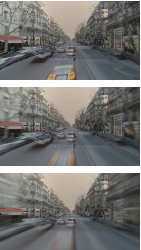
Figure 6: Screenshot of the accompanying video sequence.
The scene prior is given by the geometry of the mobile mapping system : the far plane is defined by slightly lowering (by 10cm -to get some margin) a guess of the plane of contact of the vehicle wheels and the circular paraboloid of the near plane is defined by the viewpoint location, the far plane and a radius of 10 meters at the level of the interpolated viewpoint.
The virtual viewpoint of figure 6 is generated in between two consecutive views at two thirds of the line segments joining one neighboring view to the other. The result of the projective textur-ing of these two views have been blended, as one is fadtextur-ing in and the other is fading out.
Of particular interest are the following properties : the pixels cor-responding to the direction of the motion suffer limited or no blur. Pixels away from this direction exhibit only a 1D radial blur, sim-ilar to the Star Trek-like ”hyperspace” effect. Distant and ground objects feature no aliasing, thanks to the epipolar radial blur of sufficient extent. The depth of the near surface has however been underestimated on the right of the scene, resulting in some limited ghosting of the monument. Decreasing the depth of the near sur-face enough to make it nearer than the scene at every pixel would have extended the radial blur of the pedestal in the two textures up to make their blur extent overlapping, trading out the disturb-ing double image or poppdisturb-ing artefact for an increased amount of radial blur.
4.2 Filtered Blending
3D city models of ever increasing accuracy are produced and maintained worldwide. To illustrate our method, we use a coarse 3D city model of metric accuracy (corresponding to CityGML LOD1), which is the BDTOPO c, produced nationwide by IGN, the French National Mapping Agency. The scene is composed of flat-roof buildings together with a metric accuracy Digital Terrain Model (Ground Height map). Figure 7 shows results when vary-ing the constant overall depth uncertainty parameter. A depth
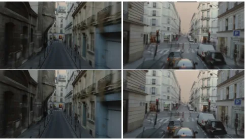
un-Figure 7: Regular filtered blending. (Top) No uncertainty has been introduced: this is only a linear blend of two 16-meter-separated textures projected on a LOD1 city model proxy. (Mid-dle) 1 meter depth uncertainty. (Bottom) 4 meters depth uncer-tainty.
certainty of 4 meters is admittedly exaggerated but shows clearly the effect of such a large depth uncertainty. Scene geometry un-certainty is only considered in the depth direction but not in the 2 others. The shortcomings of this depth-only approach is two-fold : surfaces seen at grazing angles are affected by a uncertainty that is almost coplanar with the surface, such that the uncertainty effect is underestimated. This could be prevented by taking into account the normal orientation of each pixel to compensate this underestimation. This would however only emphasize the sec-ond caveat : silhouettes remain sharp and introduce noticeable artefacts that are addressed in the following section.
4.3 Silhouette-aware Filtered Blending
Near and far surfaces may be extracted from the metric-accuracy scene of the last section using the following procedure :
2. Compute a displacement vector for each vertex of the mesh based on the normals of its neighboring triangles.
3. Add (resp. subtract) this vertex displacement attribute to the vertex locations with an overall scaling to yield the near (resp. far) surface at a given level of uncertainty.
Such a displacement vector may be defined as the average of the set of unique normal values of the adjacent triangles, tak-ing the vertical direction for the triangles originattak-ing from the DTM, the roofs and the top of the skybox and the horizontal fa-cade normal for the building fafa-cades and the skybox sides. This choice provides a 2.5D extension of the 2D mittered polygons provided by the straight skeleton (Aichholzer et al., 1995) of the building facades. Please note that step 3 does only produce valid near/far surfaces (watertight, orientable, not self intersecting with the inclusion property) for a limited range of scaling of the dis-placement field. Arbitrary uncertainty scaling may only be per-formed correctly using more complex computational geometry algorithms (de Berg et al., 1997) such as a 3D Minkowski sum and differences or a full-blown 2.5D extension of straight skele-ton algorithm that would handle topological events, conceptually performing the straight skeleton on each level set of the 2.5D mesh.
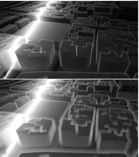
The input 3D city model used for this study used the 3D Minkowski sum approach (figure 8). Figure 9 provides a visualization of this uncertain 3D city model by displaying the normalizing factor
P
is
′
i−si. The halos around the buildings clearly show the re-gions of uncertainty and how depth-uncertainty grows at grazing angles.
Figure 10 shows how the silhouette are made uncertain by the proposed approach. A primary remark is that whereas integral radial images were only necessary for large radial blur extents, the proposed silhouette-aware extension manipulates directly its partial sums : without a precomputation technique like integral radial images, partial sums from the would have to be recomputed from scratch for every pixel over possibly long 2D line segments even for small resulting uncertainty blur. For instance the framer-ate drops from 60+ (caped) frame per second to 5 when integral radial images are disabled on our current implementation on a NVidia GPU GTX Titan.
The hard edge of the silhouette is however not fully removed. While the silhouette of the near surface produces a continuous (but notC1) result, the silhouette of the far surface still produces a discontinuous edge. Even if it is of smaller magnitude than the silhouette-unaware discontinuity, it may still be disturbing. This effect is due to our simple uniform projection density model, which causes the normalizing factor to be discontinuous as the viewing ray crosses past a far surface silhouette : this disoccludes new portions of the viewing ray which are taken into account and thus changes discontinuously the normalization factor.
5 CONCLUSIONS AND PERSPECTIVES
This paper proposed successful extensions to the filtered blending approach that provide a continuum of approaches between the geometry less set-up with a loose scene depth prior to a general set-up of an uncertain scene confined in the volume bounded by two arbitrary surfaces.
Integral radial image may prove to be of independent interest in applications that perform radial box filtering of sufficiently many pixels with the same pole. Integral radial images allowed the ef-ficient implementation of a silhouette-aware projective-texturing
Figure 8: GIS view of the uncertain 3D scene obtained by the minkowski sum (red) and difference (blue) of the original 2.5D building database (yellow). The near and far ground surfaces (MNT) are not shown here for clarity.
Figure 10: Silhouette-aware filtered blending. (Left) presents a failure case where the uncertain volume is underestimated. The protruding element is not part of the 3D model, which leads to a hard edge in the depth-uncertainty only rendering (top). The proposed approach (bottom) handles the bluring of the pixels up to silhouette of the near surfaces, resulting in a discontinuity artefact. (Right) presents a blending of the 3 nearest views with (top) depth-only uncertainty (+-1m) and with (bottom) silhouette-aware uncertainty (with the cubic structuring element[−1,1]3). Both views show similar results like the ghosting of mobile objects (pedestrians). The amount of blur in (bottom) is fully 3D and thus takes the surface normal angle into account, which produces more blur on the surfaces that are not front facing(e.g. the ground). The main difference is on the handling of occlusion boundaries (edge of the left building) which trades out the doubling artefact for a blur.
algorithm for uncertain geometry under the specific uniform pro-jection assumption.
Future work on uncertain scenes will include rendering the lidar point cloud with its measurement uncertainties and a diffusion of the depth as an uncertain interval for pixels in-between projected lidar points.
While the assumptions that led to an order-independent render-ing method with simple box-filterrender-ing enabled high performance rendering, we would like to explore the handling of the various types of occlusion and more elaborated probabilization, so that the resulting image would exactly be the probabilistic expecta-tion of the image when looking at an uncertain scene described stochastically.
ACKNOWLEDGEMENTS
This material is based upon work supported by ANR, the French National Research Agency, within the iSpace&Time project, un-der Grant ANR-10-CORD-023.
References
Aichholzer, O., Aurenhammer, F., Alberts, D. and G¨artner, B., 1995. A novel type of skeleton for polygons. Journal of Uni-versal Computer Science 1(12), pp. 752–761.
Br´edif, M., 2013. Image-based rendering of lod1 3d city models for traffic-augmented immersive street-view navigation. IS-PRS Annals of Photogrammetry, Remote Sensing and Spatial Information Sciences II-3/W3, pp. 7–11.
de Berg, M., van Kreveld, M., Overmars, M. and Schwarzkopf, O., 1997. Computational Geometry: Algorithms and Applica-tions. Computational Geometry: Algorithms and Applications, Berlin.
Eisemann, M., De Decker, B., Magnor, M., Bekaert, P., de Aguiar, E., Ahmed, N., Theobalt, C. and Sellent, A., 2008. Floating textures. Computer Graphics Forum (Proc. of Euro-graphics) 27(2), pp. 409–418. Received the Best Student Paper Award at Eurographics 2008.
Eisemann, M., Sellent, A. and Magnor, M., 2007. Filtered blend-ing: A new, minimal reconstruction filter for ghosting-free pro-jective texturing with multiple images. In: Proc. Vision, Mod-eling and Visualization (VMV) 2007, pp. 119–126.
Goesele, M., Ackermann, J., Fuhrmann, S., Haubold, C. and Klowsky, R., 2010. Ambient point clouds for view interpo-lation. Transactions on Graphics 29(4), pp. 95:1–95.
Hensley, J., Scheuermann, T., Coombe, G., Singh, M. and Lastra, A., 2005. Fast summed-area table generation and its applica-tions. Comput. Graph. Forum 24(3), pp. 547–555.