250 (2000) 23–49
www.elsevier.nl / locate / jembe
The measurement of marine species diversity, with an
application to the benthic fauna of the Norwegian continental
shelf
,1 * John S. Gray
Biologisk Institutt, Universitetet i Oslo, Pb 1064 Blindern, 0316 Oslo, Norway
Abstract
Species diversity includes two aspects, the number of species (species richness) and the proportional abundances of the species (heterogeneity diversity). Species richness and hetero-geneity diversity can be measured over different scales; a single point, samples, large scales, biogeographical provinces and in assemblages and habitats. In the literature, the terminology of these scales is confused. Here, scales are given a uniform notation. Scales of species richness and heterogeneity diversity are distinguished from turnover (beta) diversity, which is the degree of change in species composition along a gradient. Methods of measurement of the scales of species richness, heterogeneity diversity, turnover diversity and for estimating total species richness are reviewed. Two methods for measuring heterogeneity diversity are recommended Exp H9 (where
H9is the Shannon-Wiener index) and 1 / Simpson’s index, together with an equitability index J9. The reviewed methods are then applied to a data set from the Norwegian continental shelf to illustrate the advantages of the recommended methods. Finally, the application of the methods to assessment of effects of disturbance, to studies of gradients of species richness and to conservation issues are discussed. 2000 Elsevier Science B.V. All rights reserved.
Keywords: Alpha-, beta- gamma diversity; Heterogeneity diversity; Turnover diversity; Species richness
1. Introduction
The Convention on Biological Diversity (CBD) requires that its signatory nations undertake to make inventories of their biodiversity, monitor changes in biodiversity and
*Tel.: 147-2-285-4510; fax:147-2-285-4438.
E-mail address: [email protected] (J.S. Gray).
1
Present address for 2000: Department of Biology and Chemistry, City University, 81 Tat Chee Avenue, Kowloon Tong, Hong Kong. Tel.:1852-2784-4325, fax:1852 2788 7406, e-mail: bhjsgray@citvu. edu.hk 0022-0981 / 00 / $ – see front matter 2000 Elsevier Science B.V. All rights reserved.
make plans as to how biodiversity can be conserved. This is highly laudable, but makes the assumption that we know how to measure and monitor biodiversity. In the marine domain, this assumption is far from correct.
Biodiversity encompasses a range of different levels of organisation from the genetic variation between individuals and populations, to species diversity, assemblages, habitats, landscapes and biogeographical provinces. I have earlier given a general review of marine biodiversity (Gray, 1997a) but here will consider the methodological problems in measurement of the number of species and individuals in a given area.
Most studies of biodiversity are confined to the number of species in a given area, the
species richness. But the number of species alone does not describe the structure of the assemblage of species in a given area because the number of individuals per species varies. A variety of indices have been derived taking into account the proportional abundance of species (see Magurran, 1984 for a full account). These indices consider both species richness and how evenly the individuals are distributed among species (evenness or equitability). Following Peet (1974), I call this heterogeneity diversity.
Whittaker (1960) suggested that there was a range in scales of species richness. He called the number of species found in a sample alpha (or within habitat) diversity, and felt that this was the basic unit of diversity. Whittaker (1960) also suggested there was
beta (or between habitat) diversity, and species diversity measured at the largest scale he called gamma diversity. In contrast, Rosenzweig (1995) felt that the term gamma diversity was redundant since it as simply the total number of species in a biological province. Whilst Whittaker’s scheme appears to have a logic in practical terms, there are difficulties in defining and interpreting these scales. Thus, there is a need to consider these terms in detail to arrive at acceptable definitions and agreed ways to measure the different scales of species richness and heterogeneity diversity.
There are also problems when trying to compare diversity from different areas. For example when trying to publish recent papers comparing coastal with deep-sea diversities (Gray, 1994; Gray et al., 1997), the referees stated that it was not valid simply to compare coastal and deep-sea species richness. The reason given was that the deep-sea samples were always from a single uniform habitat (within habitat diversity) whereas the coastal samples were from many habitats, which the reviewers called between habitat diversity. Such an argument is wrong on two counts. First, it is quite justifiable to ask the question: are there more species in a comparable area of coastal compared with deep-sea sediment, irrespective of possible variations in the habitat? After all, it is valid to compare species richness of a tropical rain forest with that in a boreal oak-forest, even though these are different habitats. But, perhaps more important-ly, the referees had not understood what between habitat (beta) diversity really is. Whittaker (1960) defined beta diversity as the extent of species replacement or biotic change along environmental gradients. Beta diversity is not a measure of the number of species in different habitats in an area.
that in the sea scales of differences in time and space are different from those on land. Studies of marine diversity have developed their own methods and terminology that have been ignored by terrestrial ecologists. For example, Sanders (1968) rarefaction technique for comparing samples of differing size was reinvented by Coleman (1981) and gives almost identical results (Brewer and Williamson, 1994). This review analyses the above issues, proposes a uniform notation for species richness and uses some Norwegian data to illustrate approaches that can be taken.
2. Alpha, beta, gamma and epsilon diversity
Although Whittaker (1960) suggested that the most basic level of species richness was the number of species in a sample, which he called alpha diversity, he later (Whittaker, 1972) suggested that diversity could be measured at four different scales: point diversity (a single sample), alpha diversity (samples within a habitat), gamma diversity (the diversity of a larger unit, such as an island or landscape) and finally epsilon or regional
diversity (the total diversity of a group of areas of gamma diversity). Magurran (1988)
related these scales to sample, habitat, landscape and biogeographical province. Rosenzweig (1995) however, called alpha diversity ‘point’ diversity! On the other hand, Pielou (1976) stated ‘alpha diversity pertains to a small area and is a property of a particular community; even though recognition of such an entity is nearly always subjective the risk of being seriously mistaken is negligible.’
Underwood (1986) using Pielou as his source, stated ‘alpha diversity is defined as that within an identified natural community (in whatever way that is to be identified).’ Thus, Pielou and Underwood regarded alpha diversity as a property of a community, begging the question, as Underwood pointed out, of how a community should be defined. Pielou (1976) acknowledged this problem and talking of community (p 288) stated, ‘‘It should be noted that to define all the species-populations that occur together in one place as the ‘entity’ to be studied is not to assert that they constitute a ‘natural’ entity. The ‘community’ that an ecologist delimits for research purposes may prove to be clearly separated from surrounding communities by abrupt boundaries; or it may merge into them gradually and imperceptibly; or it may be clearly distinct from some but not others of its neighbours.’’ Her definition of a community is ‘several or many species-populations that occur together and interact with one another in a small region of space.’ The debate then is whether alpha diversity is a property of a community or is, as envisaged by Whittaker, the property of a sample.
If alpha diversity is a community property, then one has to assess it at the scale of a community, implying a mapping of the community first. Underwood (1986) made the same point emphatically, ‘‘What sets the angels tap dancing on the head of their pin is that beta diversity refers to spatial variability in the composition of species within a single community. There seems no way to define objectively the appropriate scale for measuring alpha diversity; there is obviously no method for distinguishing between gamma diversity (at some larger spatial scale) and alpha diversity of a community with great beta diversity.’’
biodiver-sity research, Hengeveld et al. (1997) stated that ‘‘alpha diverbiodiver-sity is the number of species occurring within an area of a given size’’. This is too broad a definition since it does not have any scale and may range from samples within a site to a biogeographical province. The latter is clearly not what is meant by alpha diversity. In a similar vein, Harrison et al. (1992) used the term alpha diversity to apply to a study of species richness within 50350 km square across UK. I believe that confusion could be avoided if alpha diversity were applied only to samples.
Statistically, there are parallels with definitions of sampling units and samples. In order to produce consistent terminology, I follow Whittaker (1965) in calling the sampling units point species richness. More sampling units taken within a broader area comprise the sample (Underwood, 1997) giving sample species richness. Sample species richness is equivalent to Whittaker’s alpha diversity. This is entirely consistent with Whittaker (1972) who stated ‘‘alpha diversity measurements are those applied to samples from particular communities’’.
2.1. Beta or turnover diversity
Although there are a number of studies of alpha diversity in a marine context, beta diversity has been almost totally neglected. Whittaker’s pioneering research (1960) compared the species richness across an altitudinal gradient in a terrestrial forest in North America. All his studies are concerned with line transects along one or more environmental gradients. Thus, his definitions and methods for measuring species richness relate to line transects and gradients. If the transect is sufficiently long, it will traverse different habitats and thus will become a between-habitat study. More usually, his transects were within one habitat. Whittaker (1975) defined beta (between habitat) diversity as: ‘‘the degree of change in species composition of communities along a gradient.’’ Whittaker stated that beta diversity ‘‘should be measured as the extent of change in, or degree of difference in composition among, the samples of a set.’’ Yet, Rosenzweig (1995), p. 33, using the framework of the equilibrium theory of island biogeography (Macarthur and Wilson, 1967) called beta diversity ‘‘the slope of the mainland species–area curve’’. This is certainly not what Whittaker had in mind since beta diversity pertains to species identities and how they change across a gradient and not with how species accumulate over areas of mainland and Rosenzweig is incorrect to suggest this as a measure of beta diversity.
From Whittaker’s definition, it is clear that beta diversity relates to the types of species contained and not to the numbers of species within two or more habitats. Magurran (1988) called beta diversity ‘differentiation diversity’ and regarded this as measuring ‘how species numbers and identities differ between communities or along gradients.’ Thus, beta diversity is not simply a measure of species richness at a larger scale than alpha diversity, but a different measure altogether. Since beta diversity is not a scale of diversity it is better to use the term turnover diversity, (Clarke and Lidgard, 1999), which is clearer.
2.2. Gamma diversity
communities, or lists of species for geographic units, or non-areal samples (such as those of light traps) drawing species from a number of communities. Pielou (1976) followed this latter idea in defining gamma diversity as pertaining to a large and almost heterogeneous collection of organisms. Likewise, Hengeveld et al. (1997) in the Global
Biodiversity Assessment, defined gamma diversity as the overall diversity within a region. But how large is ‘a large collection’ and what is meant by, ‘a region’? Rosenzweig (1995), who has a strong evolutionary background, defined gamma diversity as pertaining to a biogeographical province, making an important distinction between simply a large area and a functional evolutionary unit. The problem with such a definition is that gamma diversity applies both to a large area of unspecified size and to an evolutionary unit. I believe that it is important to separate these terms since a large area should not be confused with a biogeographical province. Terrestrial ecologists use the term landscape to cover a variety of habitats and assemblages within a given area. Whilst a term such as landscape species richness or landscape species diversity is applicable on land, it is not so easy to apply such a term to the marine environment. I suggest two scales of species richness and diversity larger than the sample scale, large
area and biogeographical province.
Spatial scaling studies are not confined to diversity issues. In terrestrial ecology, a new branch of ecology, landscape ecology, has emerged which studies scaling issues. In a marine context Thrush et al. (1999) reviewed scaling problems for soft bottom communities and have adopted the terminology of landscape ecology developed in terrestrial environments. The issues that Thrush et al. (1999) discussed are more general than species diversity and, thus, the terminology used applies more generally. Thrush et al. (1999), based on geostatistical literature, defined grain as ‘‘the area of an individual sampler, lag, the intersample distance and extent, the total area from which samples were collected.’’ Such studies usually relate to the scales of distribution of individual species and are thus at a different level to the diversity issues discussed here. As an illustration in his book on terrestrial landscape ecology, Forman (1995) used terms such as grain. ‘‘Grain refers to the coarseness in texture or granularity of spatial elements composing an area . . . . A fine-grained landscape has primarily small patches and a coarse-grained landscape is mainly composed of large patches. This scale refers to the spatial proportion of a mapped area, and grain refers to the coarseness of elements within the area.’’ Forman (1995; p. 13) defined a region as ‘‘a broad geographical area with a common macroclimate and sphere of human activity and interest. A landscape, in contrast is a mosaic where the mix of local ecosystems or land uses is repeated in similar form over a kilometers-wide area.’’ There are, of course, parallels to scales of diversity in that grain in a landscape sense covers patches of habitat within a landscape and a ‘broad geographical region’ is equivalent to large area diversity. A biogeographical province is, however, an evolutionary unit and is not found in landscape ecology definitions.
From the above analysis I believe that the confusion between terminology can be resolved if a logical series is erected. I suggest that a uniform notation can be achieved by recognising four scales of species richness: point species richness, sample species
richness, large area species richness and biogeographical province species richness. The remaining types of species richness, habitat species richness and assemblage
species richness are not scales and thus are separate measures referring to habitat or
Table 1
Proposed unifying terminology for scales of diversity Scale of species richness Definition
Point species richness: SRP The species richness of a single sampling unit
Sample species richness: SRS The species richness of a number of sampling units from a site of defined area
Large area species richness: SRL The species richness of a large area which includes a variety of habitats and assemblages
Biogeographical province species The species richness of a biogeographical
richness: SRB province
Type of species richness Definition
Habitat species richness: SRH The species richness of a defined habitat
Assemblage species richness: SRA The species richness of a defined assemblage of species
3. Measuring species richness
At the most elementary level, species richness is the total number of species in a given area. This begs the question: number of species of what? Whilst in the ideal case one would like an assessment of all species from bacteria to large flora and fauna this is impractical. Species richness more often than not refers to a single taxon, since taxonomic expertise is usually limited to specialisation in a single taxon. Ecologists working with marine sediments usually refer to the species richness of the fauna retained on a 0.5, or 1 mm sieve as macrofauna and those passing through this sieve but retained on a 0.62 mm sieve as meiofauna. Here, a size separation rather than a taxonomic division is practised in diversity studies.
Point species richness (SR ), is the number of species in a single sampling unit from aP
given area. Following Whittaker (1975), sample species richness can be measured as the
]
total number of species, SR and the mean number of species, SR based on a givenS S
number of sampling units.
Whittaker (1975) suggested that the number of species in different-sized sites can be compared by: d5SR / log A or SR / log N where SR is the total number of species inS S S
the sample, A is sample area and N is total number of individuals.
In a similar vein, Pielou (1976; p. 303) wrote: ‘‘if a comparison was to be made between the Atlantic and Pacific coasts of North America as to the diversities of the infauna of sandy beaches (in a given latitude belt), many large communities would have to be compared; censusing them would be impracticable and it would be necessary to estimate their diversities from samples.’’
Sample species richness almost certainly will be measured within a single habitat and / or assemblage, but it does not necessarily give a reliable estimate of the species richness of that habitat or assemblage. That can only be done if the extent of the habitat and / or assemblage is measured and an adequate number of samples taken to estimate species richness within that habitat or assemblage. (I prefer to use the term assemblage to community, as the former does not imply any associations between species implicit in the latter term). The total number of species in a defined habitat is therefore SR and theH
Just as with habitat and assemblage species richness, large area (SR ) and biogeog-L
raphical province species richness (SR ) estimates are made in identical ways. The areaB
covered or province boundaries have to be clearly defined and sampling design be appropriate to the scales of the features sampled.
Often there is interest in the true total number of species (SRMax) for a given habitat, assemblage, large area or province. SRMax can be estimated from species accumulation curves. Traditionally this has been done by taking the cumulative number of species on pooling samples from sample 1 to sample n, the number of samples. Yet whether or not this produces a smooth curve often depends on choice of starting sample. How should one designate the order of the samples? Whilst many simply pick a sample at random and then add the next picked at random, this does not necessarily result in a smooth curve. Today there are a number of ways of randomising samples so that one obtains a mean cumulative number of species and confidence intervals. Grassle and Maciolek (1992) used one method and we (Gray et al., 1997) randomised all samples of size one then size two and so on until the largest size is encountered. This is sampling with replacement. Colwell (1997) described a technique based on randomising without replacement. (The EstimateS programme can be obtained free at the web address: http: / / viceroy.eeb.uconn.edu / EstimateS)
Karakassis (1995) has produced a new method to estimate the total number of species in a sample. The method is based on plotting the number of species in k samples against the number in k11 samples. The intercept of the two lines gives an estimate of the total number of species in the area sampled. However, our analyses of data sets using this method showed that it grossly underestimates the true number of species (Ugland and Gray, unpubl.).
Chao (1984, 1987) has derived a rather different method for estimating total species richness for a site. The method is a non-parametric one based on the number of species with one and two individuals per species. Paterson et al. (1998) have recently applied the method to benthos from a deep sea site. Few applications of this promising method exist.
Another measure of total species richness can be obtained from Macarthur and Wilson (1963, 1967) well-known relationship between the total number of species (S ) against area (A):
Z
S5CA
where C and z are estimable parameters with C representing the biotic richness of the area and z the slope of the curve. (There are many recent reviews of species:area curves and I will not treat this topic in detail. The reader is referred to Connor and McCoy, 1979; Sugihara, 1981; Connor et al., 1983; Williamson, 1988; Lomolino, 1989; Rosenzweig, 1995; Williams, 1996; Whittaker, 1999).
Many use Arrhenius plots, species–area curves where
log S5zlog A1log C
relationship holds for a lognormal distribution (Whittaker, 1999). Both Williamson (1988) and Rosenzweig (1995) concluded from analyses of many empirical studies that the log–normal distribution is more general and therefore the log–log plot is the more usual fit. C can be used as a descriptor of the species–area relationship.
4. Measuring heterogeneity diversity
Heterogeneity diversity encompasses not only the number of species but also the proportional distribution of the individuals among the species. Indices based on the distribution of individuals among species contain additional information to that of species richness. There are many reviews of indices of species diversity and three in particular are recommended, Whittaker (1972), Hill (1973) and Magurran (1988). Following Whittaker (1965, 1972), Hill (1973) showed that, of the commonly used diversity indices, total species richness and Simpson’s index between them characterise
´
the partitioning of abundance between species; Shannon’s version of Renyi’s (1961) entropy analogy is intermediate. These three indices are those recommended for characterising species diversity.
Whittaker (1972) proposed as the first index of species diversity an index, which I call HD ,1
HD15exp(H9),
H9 is the commonly used index the Shannon-Wiener:
s
H9 5 2
O
p log pi 2 i i51where S total number of species, and pi5n /N where ni i5 number of individuals of the
ith species and N5 total number of individuals.
Whittaker (1972) also first suggested using the reciprocal of Simpson’s index (which I call HD )2
2 2 2
HD251 /( p1 1P . . .2 1p )n
where p is the proportional abundance of the first species compared to the total number1
of individuals in the n samples. Hill (1973) also used this notation. Whittaker (1972) argued that the Simpson index is primarily a measure of dominance, especially of the first 2–3 species whereas the Shannon index is more strongly affected by species in the middle of the rank sequence of species. Thus, the two indices measure different aspects of species diversity.
An additional aspect is how the abundances are partitioned among the species. This aspect has been called evenness. The most commonly used form is that of Pielou (1976):
J5H9Hmax
where H9is the Shannon-Wiener diversity index and Hmax is maximal diversity i.e. log (H ). Whittaker (1972) argued convincingly that J is not, in fact, a good measure of evenness since log S is greatly influenced by sample size, whereas H9is not. Hill (1973) suggested a new index to overcome this problem:
J9 5H9 2Hmaxor ln(HD / SR )1 S
Marine biologists have often used a version of the Pielou index as (12J ) to indicate
dominance (e.g. Gray, 1982). Recently, another method for measuring dominance has been used by Levin and Gage (1998) referred to as D and called Rank 1 dominance. It was defined as the percentage of the total fauna represented by the single most abundant species. This has been described before and is, in fact, the Berger-Parker index:
dNmax/N
where Nmax is the number of individuals in the most abundant species (Berger and Parker, 1970).
5. Turnover (beta) diversity
As mentioned earlier, turnover diversity is a different property from that of the scales of diversity. It relates to the species composition and the extent of change in, or the degree of difference in composition among, the samples along a gradient.
The simplest measure of turnover diversity is that of Whittaker (1960)
b 5 g/(a)
where g is the number of species resulting from merging a number of individual
samples and a is the number of species in a sample. For a single sample, b 51
(Whittaker, 1975) and for 2 samples that have no species in common, b 52. For three samples sharing no species, or a larger set of samples with the same total number and mean number of species as those three, b 53, implying that the extent of difference in composition among the samples of the larger set is equivalent to that in three samples with no species in common.
Two authors who have reviewed beta diversity (Magurran, 1984; Harrison et al., 1992) stated wrongly that Whittaker (1960) defined beta as:
b 5S /(a 21)
where S is the total number of species in a large area andais the number of species in a sample. Wilson and Shmida (1984) claimed that Whittaker used this version:
wherea is the average number of species found within samples. It is quite remarkable that no-one seems to have read the original paper!
Beta diversity measures the degree of change in composition of samples along a gradient, or the extent of the difference in samples from the opposite ends of a gradient. Since there are usually more than one measurement of point diversity, it is sensible to use the mean point diversity as suggested by Wilson and Shmida (1984). In the terms used here, this gives:
]
b 5S SR /(SR )S P
where SRS5 total number of species found in a sample and SR is the mean number ofP
species found within the point samples. It is, however, also possible to compare the species richness of the largest area studied with that of sample species richness:
b 5L SR /(SR )L S
In a comprehensive review, Wilson and Shmida (1984) evaluated six different measures
]
of beta diversity and concluded that the two best were Whittaker’sb 5S SR /(SR ) andS P
a new index:
]
b 5T [ g(H )1l(H )] / 2(SR )S
where g5number of species gained along the gradient and l5number of species lost along the gradient.
The two measures give very similar results. Wilson and Shmida (1984) stated thatbS
is the most widely used and does not assume a gradient structure, whereas bT
standardises by average sample richness. These two measures are currently the best measures of turnover diversity.
Harrison et al. (1992) modified Whittaker’s formula to allow comparisons of two transects of unequal size:
b 215h[S / SRS2 1] /(N2 1)j3100
where S is the total number of species in the transects, N is the number of sites, and
b 21 ranges from 0, complete similarity to 100, complete dissimilarity.
Harrison et al. (1992) also introduced a new measure for species turnover which takes account of situations where species drop out along the gradient but are not replaced by new species.
They called this index b 22:
b 225(S / SRS max)21 /(N21)3100
where SRS max is the maximal value of sample diversity in the collection of N sites.
b 22 measures the amount by which large area diversity exceeds the maximum sample diversity. These new indices have not been widely tested.
There is another way of assessing beta diversity, that is how the species similarity changes along a gradient. Pielou (1976) suggested two measures, coefficient of
statistical analyses are now in wide use in benthic ecology. Of the packages available, the Plymouth Routines in Marine Environmental Research (PRIMER; Clarke and Warwick, 1994; Carr, 1996) is widely used as is the British Natural History Museum’s BiodiversityPro (McAleece, 1997). Both calculate Bray-Curtis and other similarity indices that can be used to assess similarities between sites. Other commonly used marine programmes include NESS (Grassle and Smith, 1976; Gallagher, 1996) which has recently been used by Paterson et al. (1998) to assess similarities of fauna (beta diversity) over a depth gradient. The PRIMER package has another useful routine, SIMPER, which extracts the species that are instrumental in distinguishing between sites along a gradient. This can again be used in the context of assessing turnover diversity.
6. Comparing diversities over different scales
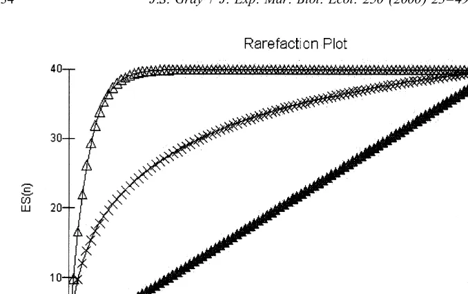
Most, if not all, indices of species diversity are sample-size dependent (Hill, 1973). Thus, in order to compare species diversities, methods are needed to reduce samples to a common size. Two methods are widely used, the rarefaction method (Sanders, 1968, corrected and modified by Hurlbert, 1971) and Coleman’s method (Coleman, 1981; Coleman et al., 1982). Both of these assume that: (a) samples are homogeneous, with similar distributions of individuals among species and (b) species are distributed randomly and are not aggregated (Brewer and Williamson, 1994). As early as 1972, Fager (1972) showed that the rarefaction method of Sanders overestimates the number of species (see also Simberloff, 1979). Surprisingly these papers have been ignored in the marine literature, although Gage and May (1993) in a paper in Nature plotted a figure (almost identical to that of Fager), showing the effect of non-homogeneity between samples.
Fig. 1 illustrates the likely sources of error in using these techniques when patterns of dominance vary. Gray et al., 1997 has shown that dominance is greater in small than in large sample sizes. This leads to the rarefaction method overestimating species richness especially at small samples. The degree of overestimation depends on the degree of dominance.
Although Fager (1972) showed the problems with the rarefaction method, it is still widely applied (e.g. Sanders, 1968; Jumars and Hessler, 1976; Rex et al., 1993; Grassle and Maciolek, 1992; Gage and May, 1993; Levin and Gage, 1998; Paterson et al., 1998; Flach and de Bruin, 1999). In many of these papers, the estimated number of species for
n individuals (ES ) was calculated for extremely small samples (e.g. only 20 or 50n
individuals). The effects of changing degrees of dominance (Fig. 1) on rarefaction estimates show that the true number of species for ES of 50 in the example given liesn
Fig. 1. Comparison of Hurlbert’s rarefaction curve (Sample 1) for data in Sanders (1968), Sample 2, all 40 species have equal numbers of individuals; Sample 3 one species with 961 individuals and 39 species each with 1 individual; after Fager (1972).
species present when species distributions deviate strongly from random’’. The problem is that nearly all species distributions depart from random. Most species have aggregated distributions and random distributions are, in fact, extremely rare in nature (Preston, 1962; Williams, 1964). Thus, rarefaction severely overestimates the species richness of small samples by making wrong assumptions concerning dominance and by assuming random rather than aggregated distributions of individuals.
It is very surprising that the rarefaction method should have taken such a large hold given these problems. An alternative, which to me seems far more logical, is to calculate species accumulation curves for randomised samples (e.g. the EstimateS programme of Colwell, 1997). This gives a mean and confidence intervals (C.I.) of numbers of species up to that of the whole sample. Plots of a series of samples of different sizes can be shown and then estimates can be given of species richness at the size of the smallest sample. If this is done then there will be a mean and 95% C.I. for each sample size smaller than the whole.
7. Taxonomic distinctiveness
which measures whether any two organisms selected at random from the full set of individuals are from the same species. Taxonomic distinctness is the expected path length of any two randomly chosen individuals from the sample, provided that they belong to different species. As yet, the method is rather new and has been applied to data sets to illustrate the value of the indices in assessment of environmental impacts rather than in diversity studies per se. Until the indices have been more widely applied, it is premature to recommend their use.
8. Applying species diversity measures to a data set
The data used to illustrate various measures of diversity are from a transect along the Norwegian continental shelf used by Gray (1994). The transect covers 1,100 km, with a total of 625 species and 40 000 individuals. The data were collected as part of the routine monitoring of the effects of the oil and gas industry. At each of the areas studied, the same sampling design was used. Sampling was at logarithmically increasing distances (250 m, 500 m, 1000 m, 2000 m and 4000 m) from the central facility, on four
2
lines at right angles to each other. At each of the sampling points five 0.1 m grab-samples were taken; the fauna remaining on a 1 mm sieve were retained and identified to species where possible. As one single grab cannot possibly be used to estimate even local species richness, the data from five grabs were pooled and such pooled data constitute the sampling unit. There were varying numbers of samples within each area. Quality control is high at all stages of the study. A species-abundance per site matrix was generated and multivariate statistics applied to measure effects of the oilrig operations on the benthic fauna (see Olsgard and Gray, 1995 for a review). In this study, only the data from samples in undisturbed sites were used. Thus, each area covered 50
2
kin , but the number of undisturbed samples within each field varied. In the Snorre area, a baseline survey was conducted before oil extraction began and, thus, this sample has the largest number of samples.
The methods described above are used to illustrate the measurement of the different scales of diversity. Biogeographical province species richness, SR , was not measuredB
since it as yet unclear where the boundaries for biogeographical provinces occur along the Norwegian continental shelf and this study was not designed to cover the biogeographical province scale. All the calculations were done using the BiodiversityPro programme (McAleece, 1997).
Table 2
Location of the areas along the Norwegian continental shelf and the basic data. Samples were taken with a 0.1
2 2
m Van Veen grab with five sampling units taken at each site giving an area of 0.5 m . The number of samples per area is thus the area divided by 0.5
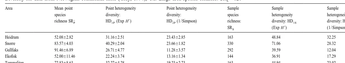
Area Lat. Long. Depth Type of Area Total no. Total no.of sediment sampled of species individuals Heidrum 658209N,078189E 305 Fine sand 12.5 163 5746 Snorre 618279N, 028089E 300 Mud 20.0 330 15 053 Gullfaks 618149N,028149E 210 Med. coarse 7.0 292 10 917 Ekofisk 568329N,038159E 72 Fine-med. Sand 4.5 144 2236 Tommeliten 568299N,028589E 70 Fine sand 5.5 620 39 582
is sensitive to the abundance of only the common species (Hill, 1973). Thus, the indices illustrate different facets of diversity.
At the sample level, Snorre has the greatest heterogeneity diversity, as measured by
H9, but drops below Heidrun using 1 / Simpson. Values are greater at the sample level since more species are encompassed in the analyses. In order to illustrate these results more clearly, plots are shown of the data beginning with species richness of the individual sampling units (Fig. 2).
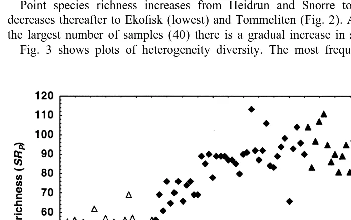
Point species richness increases from Heidrun and Snorre to Gullfaks area and decreases thereafter to Ekofisk (lowest) and Tommeliten (Fig. 2). At Snorre, which has the largest number of samples (40) there is a gradual increase in species richness.
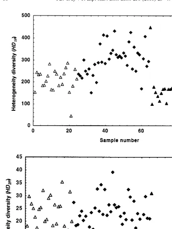
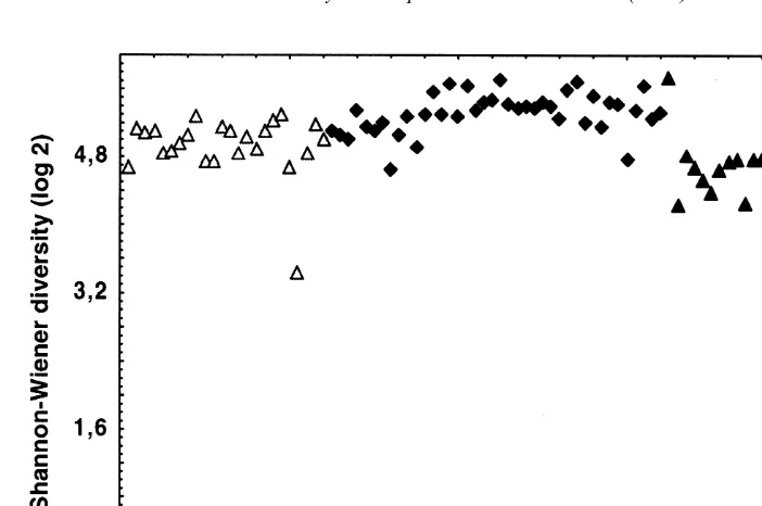
Fig. 3 shows plots of heterogeneity diversity. The most frequently used index of
Fig. 2. Plot of point species richness (SR ) for the transect, arranged in a N–S direction, as in Table 1. Key:P
.
Gray
/
J.
Exp
.
Mar
.
Biol
.
Ecol
.
250
(2000
)
23
–
49
37
Table 3
Diversity for data from Norwegian continental shelf (Gray, 1994), C.I. Large area species richness: SRL5620
Area Mean point Point heterogeneity Point heterogeneity Sample Sample Sample species diversity: diversity: species heterogeneity heterogeneity
]
Fig. 3. Point heterogeneity diversity along transect, a) Shannon-Wiener index log ; b)HD2 1P5(Exp H’); c) HDPS5(1 / Simpson’s index). Symbols as in Fig. 2.
Fig. 3. (continued )
variability and are clearly giving more information than the Shannon-Wiener index. This confirms Magurran’s (1988) view that the Shannon-Wiener is ‘less informative’ than the other indices. In these data, Gullfaks has especially small values of Exp H9 and of (1 / Simpson), whereas Ekofisk has small Exp H9but greater (1 / Simpson) than Gullfaks. Snorre has the largest values of Exp H9.
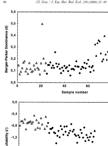
Fig. 4 shows two dominance indices, the Berger-Parker, d (Berger and Parker, 1970) and Equitability (J9 5H9 2Hmax). Both plots show very similar patterns with the greater dominance at Gullfaks (and an anomalous point at Heidrun). The equitability measure seems, however, to have more information, with a wider range of values. These data explain further why it is that, although Gullfaks has a large mean point species richness, it has small values of heterogeneity diversity because dominance is high throughout.
As mentioned in the introduction, there are almost no published studies of
differentia-]
tion (b) diversity from marine data. Table 4 shows the two scales, small (SR /(SR )S P
and large (SR /(SR ). From Table 2 the rank of sample size is SnorreL S .Heidrun.
Gullfaks.Tommeliten.Ekofisk. This pattern is in general matched in bS (Table 4), where there is an increase from small to larger scale, save that Tommeliten has a smaller value than Ekofisk and Heidrun a smaller value than Gullfaks.bL shows an interesting
Table 4
Turnover (beta) diversity calculated for sample against point species richness and large area against sample species richness and Harrison et al. (1992)b 22
]
Area b 5S SR /(SR )S P b 5L SR /(SR )L S b 22
Heidrun 3.12 3.80 2.36
Snorre 3.94 1.88 2.92
Gullfaks 3.19 2.12 2.63
Ekofisk 2.77 4.30 2.71
Tommeliten 2.23 3.80 1.86
In a recent paper, Parry et al. (1999) made the remarkable statement that ‘‘There is no adequate measure of species turnover . . . ’’ and then proceeded to use species–area curves as a direct measure of turnover diversity. Both the statement and the application are incorrect. The study was of the sediment-living fauna of four sites off the South coast of UK. Parry et al. (1999) recorded data for mean point species richness and sample species richness and it is possible to calculate turnover diversity bS. The values are Jennycliff Bay, 1.47; Cawsand Bay, 1.76; Eddystone, 2.18 and Queens Ground, 2.24. These values are smaller than the range found on the Norwegian shelf, wherebS ranged from 2.23 to 3.94, Table 2.
The only other marine data on turnover diversity are from Clarke and Lidgard (1999) who calculate values of b 22 of 1.76 to 3.29 for a latitudinal gradient of marine bryozoans. The largest values in their study were at depths between 10 and 74 m, with
smaller values at shallower and deeper areas down to 200 m. On the Norwegian continental shelf, b 22 values range from 1.86 to 2.92.
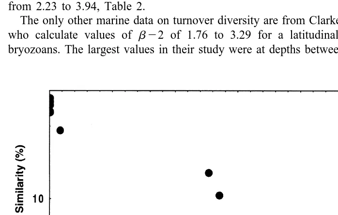
The mean similarity of the fauna within fields is 60.02% and decreases rapidly with increasing distance (Fig. 5). The similarity of the benthic fauna of the Norwegian continental shelf is halved over a distance of approximately 150 km and reduced to a quarter over approximately 400 km. For Bryozoa of the N. Atlantic, Clarke and Lidgard (1999) reported a turnover of half of the species over 450 km and 75% turnover by 5000 km latitudinally. Turnover rates are much greater for the fauna on the Norwegian continental shelf.
Finally, how does the number of species vary with area and what is the predicted total number of species along this transect? Fig. 6a shows plots using randomised cumulative species numbers against area, suggesting an asymptote at ca. 600 species. The Chao 2 estimate gives ca. 800 species (Fig. 6b). Yet it is only within the last few species that there is a tendency to reach an asymptote. The data are not unlike Grassle and Maciolek’s (1992) species accumulation curves for the fauna at 2100 m off the East coast of the US, which showed an almost linear increase in the rate of addition of species. These data do, however, represent estimates of the total number of species to be found and Grassle and Maciolek did no similar analysis. It is unlikely that 800 is a reasonable estimate. The Norwegian continental shelf has been monitored since the late 1970s and, over the years, a large data base has been built up which covers the whole continental shelf (see Gray et al. (1999) for an account). In the database, there are some 2500 species of macrofauna from the soft-sediment monitoring programme. This suggests that much larger sample sizes are needed before Chao 2 would give a reliable estimate of the total number of species. As yet there are few published studies that have used this method. Paterson et al. (1998) showed, using Chao 2, for the Domes A site in the North Pacific at 4842–5283 m depth, that the estimated total species number is around 140 species although the species accumulation curve gave ca. 100 species. They reported that at two other sites Chao 2 did not reach an asymptote.
9. Discussion
Species richness and heterogeneity diversity measures have most commonly been used to assess the impact of disturbances on the marine environment. In this context, surprisingly, much importance has been given to values of the Shannon-Wiener index. For example, in Norway the index has been incorporated into environmental legislation (Molvær, 1997). In this legislation, sediments are classified as: very good quality:
H9.4; good quality: 4–3; moderately impacted: 3–2; poor quality: 2–1; and very poor quality ,1. Fig. 3 shows that the Shannon-Wiener index is insensitive, showing little variation along the transect when compared with the other two measures (Exp H9) and (1 / Simpson’s index). In addition it has been demonstrated that use of multivariate statistics gives a much more precise way of detecting changes in benthic assemblages in space and time than use of diversity indices, (e.g. Gray et al., 1990).
equitability along the transect, with particularly small values occurring at the Ekofisk field (Fig. 4). From these data it is clear that in order to understand the biology underlying changes in species richness and heterogeneity diversity, a suite of measures are needed. In addition, it is important, in relation to the question being posed, to consider the scale over which species richness and heterogeneity diversity are measured. Too often only Point species richness, (SR ) or Sample species richness, (SR ) areP S
calculated, whereas the study was of an assemblage or habitat, where SR or SRA H are the appropriate measures. It is hoped that the review and analyses presented here may lead to a reappraisal of the appropriateness of using diversity indices alone to detect environmental change.
In the context of ecological and evolutionary theory there is great interest in patterns of species richness. Two patterns have dominated the marine literature, the latitudinal gradient and the gradient from shallow-water to deep-sea. Although the scales of these gradients are extremely large, surprisingly, most marine studies cover only a few square metres (e.g. Sanders, 1968; Rex et al., 1993; Kendall and Aschan, 1993). But what does a sample of species richness over a few square metres mean ecologically? It is well-known that species richness varies with increasing area sampled. This may be due to the fact that there are more species with increasing area, and / or there are more individuals and hence more species with a larger sample and / or that a larger area encompasses more assemblages and habitats (Rosenzweig, 1995). Yet it is valid to ask: do comparable small areas of a similar habitat in polar, temperate and tropical regions (or coasts and deep sea) have similar SRS (Gray, 1997b)? For example, Kendall and Aschan (1993) took samples off the coast of Svalbard, in Arctic Norway, off the temperate coast of Britain and in tropical Java. They found, using rarefaction, expected numbers of species (E ) for 200 individuals of 32.9Sn 61.4 (95% c.i.) species at Svalbard, 34.6 (no c.i.) in UK and 33.261.9 (95% c.i.) in Java. Since there was no difference in sample species richness between areas, they concluded that there was no evidence of a latitudinal gradient of species diversity. Yet what they sampled was SR and their studyS
shows that sample species richness does not vary with latitude.
Although Rex et al. (1993) claimed to show a latitudinal gradient in species richness of deep-sea organisms, in fact they showed that SR of two samples from the tropicsS
was greater than that of samples from temperate and polar areas. The variance between samples at any one latitude was, however, extremely large, except in the tropical area, where the two samples, by chance, had small variance. Since there is great variance between samples, this study does not give support to the idea that sample species richness varies with latitude. Recently, Levin and Gage (1998) have compared a range of SR from a variety of sites over varying latitudes and depth from the Atlantic andS
Pacific Oceans. As one might expect, SRS again showed great variance between
latitudes. The shallowest site at 108S.500 m had an ESn100 of just 5 and 9 species; at other latitudes, sample species richness varied from below 10 to over 60 species. Again, no conclusions can be drawn as to whether or not sample species richness varies with latitude.
alpha diversity for birds, which is closely related to vegetation structure, was not much higher in tropical than in temperate communities of similar structure, but beta diversity increased towards the tropics. Evolution in the tropics acts not to increase alpha diversity but to fit additional species in along environmental gradients by habitat differentiation and narrowed habitat distributions.’’ An alternative focus for marine diversity research then should be on turnover diversity rather than sample species richness. Studies of turnover diversity are potentially far more interesting ecologically than studies of sample species richness or estimates of total species richness of an area. Yet there are few marine data, a fact that Gaston and Williams (1996) lamented.
In a terrestrial study in Britain, Harrison et al. (1992) calculated turnover diversity (b 22) for a range of taxa along a N–S and E–W transect across the British Isles. They found values in the N–S transect ranging from 0.5 in moths to 3.8 in woodlice with a mean value of 1.54. For the E–W transect values ranged from 0.7 (native trees) to 6.3 (woodlice), with a mean of 3.19. Harrison et al. concluded that turnover diversity was not very great in Britain over the scales measured. The same is true for the 1000 km transect of the Norwegian coast (Fig. 5), with values equivalent to those reported for Britain. Harrison et al. (1992) report that tropical areas have turnover diversity almost an order of magnitude greater than in UK terrestrial systems. Whether or not this is true for the marine domain remains to be studied.
Recently, Clarke and Lidgard (1999) have analysed diversity of bryozoan species in the North Atlantic and found turnover diversity did not correlate significantly with latitude. There was a greater turnover at low latitudes within biogeographical provinces if one excluded data from the Mediterranean Sea. It is important to analyse how turnover diversity varies between marine taxa (as done in Harrison et al.’s (1992) study) and whether or not there are variations with size (meiofauna compared with macrofauna) and whether or not tropical areas show turnover diversity of similarly large values to those in terrestrial systems.
Likewise, there have been few studies of the species richness (SR ) of large areas inL
the marine environment. The data from the Norwegian shelf transect (Fig. 6) showed a large underestimate of the actual number of species. The predicted total number of species was 800 compared with 2500 found on the continental shelf over time (Jensen, unpublished). These data suggest that more studies are needed on species:area relationships over varying spatial scales, particularly in relation to the sizes of areas needed for sustainable conservation of marine fauna and flora.
Two studies have examined species richness at the scale of biogeographical province (SR ). Roy et al. (1996) compared latitudinal clines in species richness using a databaseB
of over 2,500 species of prosobranch molluscs. Crame (1999) has done the same with similar numbers of species of bivalves. Both showed clear clines in the Northern Hemisphere but, for prosobranchs, the greatest species richness was between 208and 308
Finally, in the Convention on Biodiversity there is a major focus on conservation of marine biodiversity. Two of the key issues relating to conservation are whether one should conserve areas of high species richness and / or areas containing many rare species. In this context Schlacher et al. (1998) have applied many of the techniques discussed in the foregoing in the to the conservation of the soft-sediment fauna of a coral lagoon. Their pioneering study examined two strategies for conservation, one based on hotspots of high diversity and one based on the conservation of ‘rare’ species. Of a total of 189 species of macrofauna, 63 were restricted to a single site (‘rare’ species) and 7 species occurred at 2 sites only. As a measure of turnover diversity, they used the number of species common to two sites for all pairwise permutations of sites and found a weak correlation with intersite distance. A single measure of turnover diversity rather than plotting each single sample point would, however, be more likely to give the pattern found in Fig. 5, with a clear relationship with distance.
In an interesting comparison, they distinguished between species restricted to a single site (‘uniques’ or spot endemics) and species represented by a single individual (‘singletons’) following the terminology of Colwell and Coddington (1994). Whereas the cumulative number of spot endemics showed a rapid approach to an asymptote, total species richness did not. This led them to the conclusions that species with small local densities dominate, distribution ranges are highly compressed (spot endemics), boundaries of assemblages overlap, there is a large turnover and a positive interspecific abundance–range size relationship. For conservation purposes, they concluded that a strategy based on total species richness would lead to missing a significant fraction of rare species. Thus, strategies based on spot endemism were the recommended approach for conserving macrofauna inhabiting sediments in this coral lagoon. Studies of other lagoons are needed to test the generality of the conclusions. The study has many useful lessons that need to be tested elsewhere.
In conclusion, it is hoped that this review will provide the stimulus for a broader approach to studies of species diversity rather than simply calculating diversity indices. Studies at all scales are urgently needed, especially in tropical regions. We do not know whether or not sample, assemblage and habitat species richness are greater in tropical then temperate or polar regions. There are few studies at larger scales than sample species richness and thus whether or not rates of species turnover are similar to terrestrial systems remains unknown. Schlacher et al.’s (1998) study showed how some of these ideas can be applied to conservation issues. Their study was, however, concerned with conservation of a part of a single lagoon. Studies that encompass larger areas, such as several lagoons within a biogeographical province, over large areas of more continuous sediment on continental shelves and on a wider range of habitats and assemblages are required if we are to use knowledge on species, assemblage and habitat richness to conserve coastal biodiversity.
Acknowledgements
edition and for his editorial skills. I thank an anonymous referee for her / his insight, which has improved the clarity and organisation of this paper. [AU]
References
Berger, W.H., Parker, F.L., 1970. Diversity of planktonic Foraminifera in deep sea sediments. Science 168, 1345–1347.
Brewer, A., Williamson, M., 1994. A new relationship for rarefaction. Biodiv. Cons. 3, 373–379. Carr, M. (Ed.), 1996. PRIMER User Manual (v4.0). Plymouth Marine Laboratory, UK, pp. 1–36. Chao, A., 1984. Non-parametric estimation of the number of classes in a population. Scand. J. Stat. 11,
265–270.
Chao, A., 1987. Estimating the population size for capture–recapture data with unequal catchability. Biometrics 43, 783–791.
Clarke, A., Lidgard S.M., 1999. Spatial patterns of diversity in the sea: bryozoan species richness in the North Atlantic. J. Anim. Ecol. (In press)
Clarke, K.R., Warwick, R.M., 1994. Change in Marine Communities: an Approach to Statistical Analysis and Interpretation. Plymouth Marine Laboratory, UK.
Coleman, B.D., 1981. On random placement and species–area relations. Mathemat. Biosci. 54, 191–215. Coleman, B.D., Mares, M.A., Willig, M.R., Hsieh, Y.H., 1982. Randomness, area, and species richness.
Ecology 63, 1121–1133.
Colwell, R.K., 1997. Estimates: Statistical Estimation of Species Richness and Shared Species from Samples. Version 5. User’s Guide and application. Published at: http: / / viceroy.eeb.uconn.edu / estimates.
Colwell, R.K., Coddington, J.A., 1994. Estimating terrestrial biodiversity through extrapolation. Phil. Trans. Roy. Soc. (Series B) 345, 101–118.
Connor, E.F., McCoy, E.D., 1979. The statistics and biology of the species–area relationship. Am. Natural. 113, 791–833.
Connor, E.F., McCoy, E.D., Cosby, B.J., 1983. Model discrimination and expected slope values in species– area studies. Am. Natural. 122, 789–796.
Crame, A., 1999. Evolution of taxonomic diversity gradients in the marine realm: evidence from the composition of recent bivalve faunas. Polar Biol. (in press).
Fager, E.W., 1972. Diversity: a sampling study. Am. Natural. 106, 293–310.
Forman, R.T.T., 1995. Land Mosaics: The Ecology of Landscapes and Regions. Cambridge University Press, Cambridge, New York.
Gage, J.D., May, R.M., 1993. A dip into the deep sea. Nature 365, 609–610.
Gallagher, E., 1996. Compah 96: A User’s Manual. University of Massachusetts, http\\:www.es.umb.edu\edgwebp.htm.
Gaston, K.J., Williams, P.H., 1996. Spatial patterns in taxonomic diversity. In: Gaston, K.J. (Ed.), Biodiversity: A Biology of Numbers and Differences. Blackwell Scientific, Oxford, pp. 202–229.
Grassle, J.F., Maciolek, N.J., 1992. Deep-sea species richness: regional and local diversity estimates from quantitative bottom samples. Am. Natural 139, 313–341.
Grassle, J.F., Smith, W., 1976. A similarity measure sensitive to the contribution of rare species and its use in the investigation of variation in benthic communities. Oecologia 25, 13–22.
Gray, J.S., 1982. Pollution effects on marine ecosystems. Neth. J. Sea Res. 16, 424–443.
Gray, J.S., 1994. Is deep-sea species diversity really so high: species diversity of the Norwegian continental shelf. Mar. Ecol. Progr. Ser. 112, 205–209.
Gray, J.S., 1997a. Marine Biodiversity: patterns, threats and conservation needs. Biodiv. Cons. 6, 153–175. Gray, J.S., 1997b. Gradients of marine biodiversity. In: Ormond, R., Gage, J., Grassle, J.F. (Eds.), Marine
Biodiversity: Patterns and Processes. Cambridge Univ. Press, Dordrecht, pp. 18–34.
Gray, J.S., Bakke, T., Beck, H.-J., Nilssen, I., 1999. Managing the environmental effects of the Norwegian oil and gas industry: from conflict to consensus. Mar. Pollut. Bull. 38, 525–530.
Harrison, S., Ross, S.J., Lawton, J.H., 1992. Beta diversity on geographic gradients in Britain. J. Anim. Ecol. 61, 151–158.
Hengeveld, R., Edwards, P.J., Duffield, S.J., 1997. Characterization of Biodiversity: Biodiversity from an ecological perspective. In: Heywood, V.H., Watson, R.T. (Eds.), Global Biodiversity Assessment. Cambridge University Press, Cambridge, pp. 88–106.
Hill, M.O., 1973. Diversity and evenness: a unifying notation and its consequence. Ecology 54, 427–432. Hurlbert, S.H., 1971. The non-concept of species diversity: A critique and alternative parameters. Ecology 52,
577–586.
Karakassis, I., 1995. S : a new method for calculating macrobenthic species richness. Mar. Ecol. Progr. Ser.8
120, 299–303.
Kendall, M.A., Aschan, M., 1993. Latitudinal gradients in the structure of macrobenthic communities: a comparison of Arctic, temperate and tropical sites. J. Exp. Mar. Biol. Ecol. 172, 157–179.
Levin, L.A., Gage, J.D., 1998. Relationships between oxygen, organic matter and the diversity of bathyal macrofauna. Deep-Sea Res. 45, 129–163.
Lomolino, M.V., 1989. Interpretations and comparisons of constants in the species–area relationship: an additional caution. Am. Natural. 133, 277–280.
Macarthur, R.H., Wilson, E.O. (Eds.), 1967. The Theory of Island Biogeography. Princeton Univ. Press, Princeton. N.J, pp. 1–203.
Magurran, A., 1988. Ecological Diversity and its Measurement. Croom Helm, London. McAleece, N., 1997. BioDiversityPro. (http: / / www.nrmc.demon.co.ukibdpro / )
Molvær, J., 1997. Classification of environmental quality in fjords and coastal waters. A guide. Statens forurensingstilsyn. 97 (03) SFT Oslo, pp 1–34.
Olsgard, F., Gray, J.S., 1995. A comprehensive analysis of the effects of offshore oil and gas exploration and production on the benthic communities of the Norwegian continental shelf. Mar. Ecol. Progr. Ser. 122, 277–306.
Paterson, G.L.J., Wilson, G.D.F., Cosson, N., Lamont, P.A., 1998. Hessler and Jumars (1974) revisited: abyssal polychaete assemblages from the Atlantic and Pacific. Deep-Sea Res. 45, 25–251.
Peet, R.K., 1974. The measurement of species diversity. Ann. Rev. Ecol. System. 5, 285–307. Pielou, E.C. (Ed.), 1976. Population and Community Ecology. Gordon & Breach, Chicago, pp. 1–424. Preston, F.W., 1962. The canonical distribution of commonness and rarity, of species. Ecology 29, 254–283.
´
Renyi, A., 1961. On measures of entropy and information. In: Neyman, J. (Ed.), 4th Berkeley Symposium on Mathematical Statistics and Probability, Berkeley, pp. 547–561.
Rex, M.A., Stuart, C.T., Hessler, R.R., Allen, J.T., Sanders, H.L., Wilson, G.D.F., 1993. Global-scale latitudinal patterns of species diversity in the deep-sea benthos. Nature 365, 636–639.
Rosenzweig, M.L. (Ed.), 1995. Species Diversity in Space and Time. Cambridge University Press, Cambridge, pp. 1–436.
Sanders, H.L., 1968. Marine benthic diversity: a comparative study. Am. Natural. 102, 243–282. Steele, J.H., 1985. A comparison of terrestrial and marine ecological systems. Nature 313, 355–358.
Z
Sugihara, G., 1981. S5CA , z51 / 4; a reply to Connor and McCoy. Am. Natural. 117, 790–793. Thrush, S.F., Lawrie, S.M., Hewitt, J.E., Cummings, V.J., 1999. The problem of scale: Uncertainties and
implications for soft-bottom marine communities and their assessment of human impacts. In: Gray, J.S., Ambrose, W., Szaniawska, A. (Eds.), Biogeochemical Cycling and Sediment Ecology NATO ARW. Kluwer Scientific, Dordrecht, pp. 195–210.
Underwood, A.J., 1986. What is a community. In: Raup, D.M., Jablonski, D. (Eds.), Patterns and Processes in the History of Life. Dahlem Konferenzen 1986. Spinger-Verlag, Berlin, Heidelberg, pp. 351–367. Underwood, A.J., 1997. Experiments in Ecology: Their Logical Design and Interpretation Using Analysis of
Variance. Cambridge University Press, Cambridge.
Vetter, E.W., Dayton, P.K., 1998. Macrofaunal communities within and adjacent to a detritus-rich submarine canyon system. Deep-Sea Res. 45, 25–54.
Warwick, R.M., Clarke, K.R., 1998b. Taxonomic distinctness and environmental assessment. J. Appl. Ecol. 35, 532–543.
Whittaker, R.H., 1960. Vegetation of the Siskiyou Mountains. Oregon and California. Ecol. Monogr. 30, 279–338.
Whittaker, R.H., 1965. Dominance and diversity in land plant communities. Science 147, 250–260. Whittaker, R.H., 1972. Evolution and measurement of species diversity. Taxon 21, 213–251.
Whittaker, R.H. (Ed.), 1975. Communities and Ecosystems, 2nd Edition. Macmillan, New York, pp. 1–385. Whittaker, R.J., 1999. Island Biogeography; Ecology, Evolution and Conservation. Oxford. University Press,
Oxford.
Williams, C.B., 1964. Patterns in the Balance of Nature and Related Problems in Quantitative Ecology. Academic Press, London.
Williams, M.R., 1996. Species: area curves: the need to include zeroes. Global Ecol. Biogeogr. Lett. 5, 91–93. Williamson, M., 1988. Relationship of species number to area, distance and other variables. In: Myers, A.A., Giller, P.S. (Eds.), Analytical Biogeography, An Integrated Approach to the Study of Animal and Plant Distributions. Chapman and Hall, London.