Semiparametric identi
"
cation and
heterogeneity in discrete choice dynamic
programming models
Christopher R. Taber
Department of Economics and Institute for Policy Research Northwestern University, 2003 Sheridan Road, Evanston, IL 60208, USA
Received 1 January 1997; received in revised form 1 June 1999
Abstract
Empirical discrete choice dynamic programming models have become important empirical tools. A question that arises in estimation and interpretation of the results from these speci"cations is which combination of data and assumptions are needed to overcome problems of heterogeneity, selection, and omited variables bias. This paper addresses this question by considering nonparametric identi"cation of a version of the model that allows for quite general forms of unobservable and information structures. I show that the model can be identi"ed under conditions similar to a static poly-chotomous choice model. Using a stochastic version of an &identi"cation of in"nity' argument, utility can be identi"ed up to a monotonic transformation of the observables under strong support conditions and two types of exclusion restriction. The"rst type is similar to a standard static exclusion restriction: a variable that in#uences the"rst period decision, but does not enter the second period decision directly. The second type requires a variable that does not a!ect the utility of the"rst option directly, but is known during the"rst period, and has predictive power on the choice during the second. I also provide two speci"cations under which the full error structure can be identi"ed. This requires the additional assumption of stochastic innovations in the observables. I then use the model to estimate schooling decisions in which students deciding whether to drop out of high school account for the option value of attending college. ( 2000 Elsevier Science S.A. All rights reserved.
JEL classixcation: C14; C35; C51
Keywords: Identi"cation; Discrete choice; Dynamic programming
1. Introduction
Empirical discrete choice dynamic programming models have become impor-tant empirical tools. In some applications of these models, problems of substan-tial heterogeneity/selection/omitted variable bias arise (see, e.g. Keane and Wolpin (1997) or Eckstein and Wolpin (1997)). The source of these biases is potentially more complex in dynamic models than static ones in that agents may have heterogeneity not only in outcomes, but also in expectations about future outcomes. A question that arises in estimation and interpretation of the results in these cases is which combination of data and assumptions are needed to overcome these problems. This paper addresses this question by considering nonparametric identi"cation of a version of the model that allows for quite general forms of unobservable and information structures. Despite the added complexity of the model, I show that it can be identi"ed under conditions similar to a static polychotomous choice model. Using a stochastic version of an
&identi"cation of in"nity'argument, utility can be nonparametrically identi"ed up to a monotonic transformation of the observables under strong support conditions and two types of exclusion restriction. The "rst type is similar to a standard static exclusion restriction: a variable that in#uences the"rst period decision, but does not enter the second period decision directly. The second type requires a variable that does not a!ect the utility of the"rst option directly, but is known during the"rst period and has predictive power on the choice during the second. I also provide two speci"cations under which the full error structure can be identi"ed. This requires the additional assumption of stochastic innova-tions in the X's: a variable known at time one that helps predict the second period decision, but conditional on second period observables, has no in#uence on the decision.
college. Accounting for this type of heterogeneity in information requires a more complex information structure about unobservables than is often used in em-pirical work. This leads to two important questions (1) can an information structure such as this be identi"ed? and (2) if not, can other important structural parameters be identi"ed without this information? I provide a set of conditions under which the coe$cients can be identi"ed allowing for these forms of unobserved heterogeneity in information about the unobservables. While we can not identify an arbitrarily complicated information structure under stan-dard conditions, I provide two speci"cations under which we can.
Discrete choice dynamic programming models have been applied to a large range of topics. Examples include patent renewal (Pakes, 1986), bus engine replacement (Rust, 1987), job search (Wolpin, 1987), fertility (Hotz and Miller, 1993), life cycle earnings (Keane and Wolpin, 1997), and schooling (Taber, 1998); a survey can be found in Eckstein and Wolpin (1989) or Rust (1994). The main goal of this paper is to establish identi"cation of these models under fairly weak assumptions about the distribution of the error and information structure. These results are useful for two reasons. First, they take a "rst step towards semiparametric estimation of this class of models by establishing su$cient conditions for their identi"cation. To facilitate estimation, this work typically imposes strong parametric restrictions on the distribution of the unobservables and on the information structure that agents use to form their expectations. These assumptions are typically chosen out of mathematical convenience rather than as implications of the models themselves so it is important to check the sensitivity of the model to these assumptions. Secondly, and perhaps more importantly given current computational problems, they demonstrate the ideal data set under which these models can be identi"ed without parametric restric-tions. Solving the heterogeneity bias problem can typically be achieved by imposing functional forms on the distribution of the error terms. However, it is preferable to"nd data that can solve the problems. In practice the perfect data set rarely exists, so identi"cation is achieved through a combination of data and assumptions. Nevertheless, this type of identi"cation exercise is potentially useful both for understanding the trade-o!between assumptions and data and for illuminating which type of data one should use when estimating these models.
While much work has been done on semiparametric identi"cation of other discrete choice models, it has not been systematically discussed in dynamic programming problems. There have been a few papers that focus on speci"c points, often with negative results. Flinn and Heckman (1982) consider
1They do not explicitly talk about identi"cation at in"nity, but in their notation send a second period variablec
2above>Jwhere>Jis the upper bound of the support of the second period error
term.
models. The most closely related work is by Pakes and Simpson (1989). They provide a sketch of identi"cation for a"nite period model of patent renewal that could be written as a special case of mine. They also use exclusion restrictions and essentially a similar identi"cation at in"nite argument.1I extend this model into a broader framework by allowing for a more general form for unobser-vables and information, and a more general process for the obserunobser-vables. Cameron and Heckman (1998) also consider identi"cation of schooling models, but the form of their models are quite di!erent in that they do not use this dynamic programming framework.
This paper extends the work on identi"cation of discrete selection models in static cases to incorporate dynamics. As in this paper, most of the previous work generalizes the ideas behind the semiparametric identi"cation of the binary choice model,
d"1(g(X, h)#e'0). (1)
The functiongis assumed known up to parameterh, but the distribution ofeis unspeci"ed. Identi"cation of this simple model is presented in Cosslett (1983) and Manski (1975,1988). Extensions that allow for multiple choices or multiple periods include Manski (1987), Thompson (1989), Cameron and Heckman (1998), and Cameron and Taber (1994). Matzkin (1990,1992,1993) follows an-other line. She extends the semiparametric identi"cation to nonparametric identi"cation. For instance in the binary choice model (1) she allows
g(X, h)"g(X) and provides conditions under which the functiongis identi"ed. I describe the model in Section 2. I provide identi"cation of various compo-nents of the model in Sections 3 and 4. In Section 5 I demonstrate how these results can be used by estimating a version of the model as a schooling model where a student"rst decides whether to graduate from high school and then conditional on high school graduation decides whether to attend college. Sec-tion 6 presents some conclusions.
2. Model and notation
2This assumes that at the time of graduation the student recognizes she will receive this utility later in life.
forward. The model consists of two time periods and three terminal states. It can be thought of essentially as a dynamic extension of the Roy model (Roy, 1951; Heckman and HonoreH, 1990). The structure takes the following form,
In the "rst period the agent chooses between node a and node ac. If she chooses nodeacin the"rst period, she then chooses between nodesbandcin the second. In a schooling model node a could represent dropping out of high school, nodebgraduating from high school and entering the labor force, and node cgraduating from college. When making the decision to graduate from high school the student does not know her college options with perfect certainty.
The agent's preferences are summarized by lifetime reward function<
kat each
terminal state k3Ma,b,cN. By de"ning utility at the terminal nodes, I do not separate utility at nodeacfrom utility at nodesbandc. Rust (1994) essentially shows that one can never distinguish utility incurred at node ac from utility incurred at node b and c, but known with perfect certainty at time 1. The intuition behind this is clear in the schooling example in which it is impossible to tell whether the utility accumulated from graduating from high school actually is realized during the graduation ceremony or whether it accrues later in life while looking at the degree on the wall.2In an in"nite time model this type of normalization is not possible, so the potential problem is more severe.
I de"ne<
aso that it is known at the time the choice betweenaandacis made
and<
b and<c are known at the time the choice betweenbandcis made. Let
I
1denote the information available to the agent at the time of the"rst decision. I assume that decisions are made in order to maximize expected lifetime reward. Thus the reward function at nodeacin the"rst period takes the value,
<
ac(I1),E[maxM<b,<cN DI1]. The agent chooses nodeaif<
a'<ac(I1), and chooses nodeacotherwise. If she choosesacin the"rst period, she chooses nodebin the second if<
b'<c.
3An unappealing feature of this type of model is the separability and independence between the observables and unobservables. This assumption is chosen out of convenience, not as an implication of economic theory. Unfortunately, something analogous to it is necessary for identi"cation. I use this speci"cation for its simplicity and for direct comparison with previous work. The proofs in this paper can be easily altered to address other types of restrictions that have been used for the binary choice model.
certainty, the agent would simply choose the alternative with the highest lifetime value function and the model would be identical to the standard polychotomous choice problem. The basic structure of the speci"cation I present below is similar to the polychotomous choice models of McFadden (1981), Thompson (1989), or Matzkin (1993). The model di!ers from these others only in that during the"rst period the agents are uncertain about their utilities in the second.
The econometrician observes (d
a,db,dc,Xa,Xb), where fork"Ma,b,cN,dk is
an indicator that statekwas chosen. I de"ne them explicitly as,
d
a"1(<a'<ac(I1)), (2)
d
b"1(<a)<ac(I1),<b'<c), (3)
d
c"1(<a)<ac(I1),<b)<c), (4)
where 1()) is the indicator function taking the value one if its argument is true and zero if it is false.
I de"ne the reward functions at each terminal node to take the following form:
<
a"ga(Xa)#ea, (5)
<
b"gb(Xb)#eb, (6)
<
c"0. (7)
Since utilities are identi"ed only up to monotonic transformations I normalize utility at nodecto zero (see Taber, 1996, for justi"cation). The functionsg
aand
g
b may be"nite dimensional as in Manski (1975) or Cosslett (1983) or in"nite
dimensional as in Matzkin (1990). The random vector (X
a,Xb) is observed by
the econometrician and independent of the unobserved random vector (e a, eb).3
The joint distribution of the error terms are left unspeci"ed. I allow the information setI
1 to be heterogeneous across individuals and do not restrict private information that is contained inI
1to be independent of the error terms. To simplify the exposition I assume that the "rst period information about
e
4By assuming thatX
1is observable, I do not allow the agents to be better at forecasting their future values ofX
bandXcthan the econometrician. This assumption is not crucial for the results in
Section 3, but would complicate identi"cation of the full model in Section 4. 5In other words, I can construct some functionasuch thatX
a"a(X1), but in general I cannot "nd a functiona~1such thatX
1"a~1(Xa).
we may want to think of it as a very large dimensional vector. All that is relevant aboute1 is the information it provides. Similarly, the"rst period information aboutX
bis completely contained in the observable random vectorX1.4Thus, I
1"p(e1, X1),
where the notation p(>) denotes the sigma algebra generated by a random
variable>. In addition, I assume that the observables (X
1,Xa,Xb) are
indepen-dent of the unobservables (e1, e a, eb).
Since the agents know the value ofX
a during the"rst period, p(X
a)Lp(X1). I am not requiring thatX
a"X1, only that knowledge of X1 is su$cient for knowledge ofX
a.5Similarly I do not assume thatea"e1, only that
p(e
a)Lp(e1),
thus the agent may have private information about the values of future unobser-vables that is not contained inp(e
a).
The structure is summarized in the following table:
Known to the Agent Learned by the Observed by the at time one Agent at time two Econometrician
e1,e
Proving identi"cation involves showing that the functions (g
a,gb) and aspects
of the joint distribution of (e1, e
a, eb) are identi"ed from the observed
condi-tional probabilities. I also allow common shocks to occur between period one and period two. I denote the outcome of these shocks by W
The consequences of these types of shocks is to cause the ex-ante conditional distribution of (e
bD e1) which agents use to form<ac to di!er from the ex-post realization of (e
bD e1,W2). This could also represent departure from rational expectations. The econometrician observes Pr (aDX
1) and Pr (bDX1,Xb,W2), de"ned as,
Pr (d
a"1DX1)"Pr(ga(Xa)#ea'<ac(X1,e1)DX1) (8) Pr (d
b"1DX1,Xb,W2)"Pr (ga(Xa)
#e
a)<ac(X1, e1),gb(Xb)#eb'0DX1,Xb,W2). (9) The goal of this work is to provide conditions under which (8) and (9) are su$cient for identi"cation of the functions (g
a, gb) and the joint distribution of
the unobservables (e1, e a,eb).
As mentioned above, there is an aspect to this problem that di!erentiates it from most previous work on both static and dynamic discrete choice models. Sincee1 is person speci"c, the function<
ac(X1, e1) is also person speci"c. This represents a di!erent type of heterogeneity: heterogeneity across expectations as opposed to heterogeneity across outcomes. The only restriction imposed on information heterogeneity is that an agent's time one expectations of e
b are
independent of the observablesX"(X
1,X2).
3. Identi5cation ofgaandgb up to monotonic transformations
In this section I provide conditions which deliver identi"cation of g
a and
g
bwith minimal assumptions about the distribution of the unobservables. I use
a de"nition of identi"cation that is analogous to Matzkin (1992). By identi" ca-tion of g
a and gb up to a monotonic transformation, I mean that for any
alternative functions and distribution of error terms (gH
a, gHb, eHa, eH1, eHb)
consis-tent with the observed probabilities,
Pr [g
a(Xa)#ea'<ac(X1, e1)DX]"Pr [gHa(Xa)#eHa'<aHc(X1,eH1)DX] and
Pr[g
a(Xa)#ea)<ac(X1,e1),gb(Xb)#eb'0DX,W2]
"Pr [gH
a(Xa)#eHa)<Hac(X1, eH1),gHb(Xb)#eHb'0DX,W2],
gHa andgHb must be monotonic transformations ofg
a andgb. That is it must be
the case that for almost any (x1b,x1a,x2b,x2a) if
g
then
gH
b(x1b)'gHb(x2b), gHa(x1a)'gHa(x2a).
I"rst present the conditions required for identi"cation, pose the theorem, and then describe the general strategy of the proof. The notation suppM>Ndenotes
the support of random variable>. SinceX
a is measurable with respect toX1, the notationX
a(X1) denotes that value ofXa consistent withX1.
Condition G1. For any x
b3suppMXbNandx13suppMX1N, suppMe
aN"(S-ea,S6ea)LsuppM!ga(Xa)DXb"xb)N, suppMe
bN"(S-eb,S6eb)
(S-ea,S6ea,S-eb, andS6eb need not be"nite)
Condition G2. For anyx
a3suppMXaN, y3(!S-eb,!S6eb), andc3(0,1), there exists a setX
1(xa,y,c) with positive measure such that forx13X1(xa,y,c),
(a) x
a"Xa(x1), (b) Pr (g
b(yDX1"x1)'c, (c) The distribution ofg
bconditional onx1is stochastically dominated by the unconditional distribution ofg
b.
Condition G3.
E(De
bD D e1)(R and E(Dgb(Xb)D DX1)(R.
Theorem 1. Under Assumptions G1,G2, and G3,g
a and gb are identixed up to
monotonic transformations within (!S6ea,!S-ea) and (!S6eb,!S-eb) respectively
(Proof in Appendix).
The basic strategy used in this proof is a stochastic extension of&identi"cation at in"nity'. This type of approach is common in static models (see, e.g. Chamber-lain (1986), Heckman (1990), Matzkin (1993), or Cameron and Heckman (1998)) and is very di$cult to avoid in these types of selection models without paramet-ric restparamet-rictions on the distribution of the unobservables. To see how this type of approach works and why it is almost necessary, consider a standard selection model where,
d"1(Z#e'0), y"b
0#u,
6And similarly if we could condition onZso that Pr (d"1DZ) is&close'to one then we could obtain an estimate&close'tob0.
7Heckman and Vytlacil (1999), Aakvik et al. (1999), and Ichimura and Taber (1999) use a di!erent strategy. They consider the case where one has exclusion restrictions for this problem, but not full support ofZ. In this case one cannot get point estimates ofb0but can get bounds on these values. A similar strategy could be used for the model presented here as well.
that Pr (d"1DZ"zH)"1 then we could identifyb0since E(>DZ"zH)"b
0.6 We could then trace out the joint distribution of (e,u) by varyingZ.
Two assumptions are important for this strategy. (1) We need an exclusion restriction (a variableZ) that enters the selection equation, but not the regres-sion equation, and (2) this variable must have a large support. To see why this second assumption is hard to avoid suppose the support ofZis bounded above byZM where Pr (d"1DZ"ZM)(1. In this case for any e(!ZM, d"0 and y
is unobserved. This means that the data is completely uninformative about E(uD e(!ZM ). Without information about this object, the assumption E(uDZ)"0 will not su$ce to identifyb0.7To achieve nonparametric identi" ca-tion ofb0without placing strong conditions on the conditional distribution ofu, some type of&identi"cation at in"nity'strategy cannot be avoided.
My model has a similar selection structure. The econometrician can only observe the decision between band cfor individuals who reject a. The same intuition for identi"cation that comes from the standard selection model will hold in this case. We typically possess less information in a discrete choice model than in a selection model so it is very di$cult to avoid the&identi"cation at in"nity'strategy here as well without strong restrictions on the error terms.
I identifyg
b in almost exactly the same manner asb0in the above example. With an exclusion restriction we can condition ong
aarbitrarily low so that the
probability of selecting node ais close to zero. This leaves us with a simple binary choice model in which the agents choose betweenbandc. From previous work we know in this case that we can identifyg
bup to a monotonic
transforma-tion. The type of exclusion restriction used here is a variable that entersg
a, but
does not in#uenceg
b directly. To see this suppose thatXa is unidimensional,
8I assumed one piece of information that is not available. I assumed that the econometrician knew thatg
awent to negative in"nity withxaeven though I have not shown thatgais identi"ed.
This is not a serious issue since holdingg
bconstant, the set ofxafor whichgaP!Ris the same as
the set ofx
afor which the probability of choosingagoes to zero which is observable.
Using standard identi"cation strategies for the binary choice model (see, e.g. Manski (1988) or Matzkin (1992)), I can identifyg
b.8If we have a variable that
in#uencesg
a, but notgbdirectly then we can"xXband still varyga. This type of
exclusion restriction satis"es G1. Note that time varying X's are typically su$cient for an exclusion restriction here. A"rst period outcome will in#uence
g
a, but not inIdenti"cation of#uenceg gb conditional on the second period outcome.
ais somewhat trickier. Since the sequencing of the choices is
di!erent, at "rst glance the problem does not seem to take the form of the selection model. However, it is similar. Since <
c is normalized to zero,
g
a represents the di!erence in utility between a and c that is made given
information at time 1. If we could condition on a group of people for whombis not an option, then we could identify g
a using the same argument as above.
Since in generalg
bwill depend on values ofXbthat are not realized until time
two we cannot condition ong
bat time one. Instead I develop a stochastic notion
of identi"cation at in"nity. Rather than conditioning on a set ofX
b such that
g
bis small, I condition on a set ofX1 such that the conditional distribution of
g
bThis requires a somewhat diis&small.' !erent type of exclusion restriction, a variable
known at time one that does not enter g
a directly, but does have predictive
power for the distribution ofg
babove and beyondXa. To see how this works,
suppose we have a variableX
1that satis"es these conditions and that asx1gets small the conditional distribution ofg
b becomes small. In this case
lim
From this piece we can identifyg
aup to a monotonic transformation. This type
of variable will satisfy G2. Note that simple time varyingX's will not typically be su$cient in this case. We need a variable that is known at time one and does not enter g
a directly. A second period realization of an observable will not enter
g
Given a set of exclusion restrictions with large enough support, the model is essentially transformed from a dynamic model to a static binary choice model. Thus, the identi"cation strategy here can be easily extended to other cases addressed in that literature. For example, if one wanted to allow for hetero-skedasticity in the error terms as in Manski (1975), a combination of Assump-tions G1 and G2 as well as Manski's assumptions would be su$cient for identi"cation. Extending the model to more periods and more choices is also straight forward. With multiple choices one needs multiple exclusion restriction that would be jointly sent to in"nity. Once again it would be almost impossible to nonparametrically identify the model without this type of assumptions. Extending the model to allow for endogenous continuous variables in a manner similar to Heckman and HonoreH (1990) was done in Taber (1996). It also uses the intuition presented here.
The assumptions above about access to exclusion restrictions can be relaxed if one is willing to make parametric assumptions about g
a and gb. In
parti-cular if g
a"X@ba and gb"X@bb, then exclusion restrictions are no longer
necessary (see Taber, 1996). To see the intuition for this, as long as b a is not
proportional tob
b we can sendgaPR, and still have enough variation inXto
identifyb b.
4. Identi5cation of the distribution of the unobservables
The theorems above show that g
a and gb can be estimated even if we can
say nothing about the distribution of the error terms. However, their nonparametric identi"cation is of interest as well. Typically these types of structural models are estimated with the goal of simulating policy counterfac-tuals. Except in very special cases, without knowledge of the full model, these counterfactuals cannot be constructed. For example, in the schooling case, suppose that policy makers consider subsidizing college education. Evalu-ating the consequences of the policy on schooling outcomes from the model cannot be done usingg
aandgb alone. A second reason for exploring identi"
ca-tion of the distribuca-tion of unobservables is that nonparametric identi"cation of the unobservables is required for the use of many semiparametric estimators. For example, showing consistency of the nonparametric maximum likelihood estimator that I use below requires identi"cation of the distribution of the unobservables. Finally, the joint distribution of the unobservables may be of interest in its own right. In the schooling model a researcher may be interested in understanding the manner in which students learn about their own ability.
Assumption E1. For ally3R, Pr[e
Assumption E1 eliminates the possibility of a di!erence between the ex-ante and ex-post conditional distribution ofe
b. It is helpful for identi"cation because
it places strong restrictions on the relationship between the conditional distribu-tion ofeb and the conditional distribution agents possess abouteb during the
"rst time period. Without this assumption, or at least a strong restriction on the way these e!ects operate, identi"cation of the full model from only one realization ofW
2 is not feasible.
Assumptions E2 and E3 are alternative conditions on the"rst period informa-tion people possess about their unobservables. Neither is stronger than the other. Assumption E2 essentially allows for general types of serial correlation. It imposes that agents have no information about e
b beyond ea, but does not
restrict the relationship betweene
aandeb. Assumption E3 allows a very general
conditioning set, but restricts the knowledge of e
b to be simply its expected
value. In the schooling model one might expect that individuals have more information about their returns to college than is conveyed through their returns to high school, so Assumption E3 is probably more appropriate. How-ever, in cases in which the decision between aand ac is similar to the choice betweenbandc, Assumption E2 may be preferred.
The "rst result of this section is that even under the seemingly strong conditions above, identi"cation of the error structure cannot be achieved with-out stochastic innovations in the observables between the two periods. That is, when agents know the value of X
b with perfect certainty in the "rst period,
identi"cation cannot be achieved even under strong parametric assumptions. The basic problem is that the choice in the "rst period is in#uenced by
<
ac(X1, e1). If Xb were known with perfect certainty in the "rst period then
X
1"Xb and we could not vary gb(Xb) separately from <ac(Xb, e1). Under Assumption E3, that would leave us with essentially two degrees of freedom (g
a,gb) to identify a three dimensional distribution (ea, lb, gb). Under
Assump-tion E2 the intuiAssump-tion is more subtle. Sinceg
b(Xb) enters both the"rst and second
period decisions, it is not possible to di!erentiate between the two roles which is necessary for identi"cation in some cases.
I"rst use counterexamples to demonstrate nonidenti"cation of the distribu-tion of the error terms in this case. I then show that with stochastic innovadistribu-tions inX
conditions will rule them out. Unless we use these other very strong assump-tions, stochastic innovations in the observables between periods are necessary for identi"cation.
In what follows I assume thatg
a and gb are identi"ed. In the"rst section
I showed that they could be identi"ed up to monotonic transformations. Therefore, after choosing a class of functions which are normalized up to a monotonic transformation, they are identi"ed. There are a number of di!erent normalizations have been used in the binary choice model that can be used here as well (see, e.g. Manski (1988), Cosslett (1983) or Matzkin (1990,1992)). I will not discuss speci"c ones but refer the reader to previous work. The only somewhat unique aspect of this problem is that we can only normalize one of these functions, and given this normalization the other should be identi"ed. For example in the linear case if we normalize the scale ofg
awe can identify the scale
ofg
bunder the conditions presented in the previous section. In some cases when
g
a and gb are completely nonparametric this identi"cation requires an
addi-tional exclusion restrictions (a variable that in#uences g
c, but not ga or
g
b directly). These issues are much easier to deal with under speci"c forms of
g
aandgb rather than in the general case, so for the sake of space, I just assume
these conditions hold rather than get into these details.
Assumption G4.g
a(Xa) andgb(Xb) are identi"ed.
I "rst consider the case in which X
b is known to the agent with perfect
certainty during the "rst period, so E(g
bDX1)"gb. Notice that when
b. The problem is that we cannot identify the joint
dis-tribution.
I"rst show through a counterexample that Assumptions E1 and E2 are not su$cient for identi"cation in the case whereX
bis known during the"rst period.
The basic intuition is that we do not have enough variation in the observables to separate the direct e!ect of e
a from its role in predictingeb.
Counterexample 1. Assume thateais binomial and that the distributioneb
condi-tional on ea is also binomial for each value of ea. I let the (ea,eb) have the following distribution,
e a"
G
h1 with probabilityo,
(e
a"/3and/b"/4cannot be distinguished from an alternative model with/
a"/4 and/b"/3.
Now consider Assumption E3. I will go to the two extremes and provide a counterexample in which I cannot distinguish a model in which the agent has full knowledge ofe
bduring the"rst period (i.e.eb"lb) from a model in which
the agent has no knowledge ofe
b during the "rst period (i.e. eb"gb). I take e
a and eb to be distributed logistically and show that the nested logit model
cannot be distinguished from a model in which agents have no information aboute
bat time one. McFadden has shown that the nested logit can be derived
from a multinomial choice model. These models are special cases in which the agents have full information in the"rst period.
Counterexample 2. I present the models in the context of my current notation
without the normalization ofg
c"0. I letg(kbe the original reward functions so
by de"nitiong
a"g(a!g(c andgb"g(b!g(c. The following two models produce
the same choice probabilities.
Model 1 (Nested Logit Model(McFadden 1977,1981))
In other words the error terms are all independent with Type 1 extreme value distribution.
Now suppose that X
b is not known with perfect certainty during the "rst
period. In this case it is possible to provide su$cient conditions under which the distribution of the unobservables is identi"ed. I assume E1 and show that either E2 or E3 are su$cient for identi"cation. I use the following additional assump-tion,
Condition G5. For almost allx13supp(X1), (Se-b,S6eb)3supp(!g
b(Xb)DX1"x1). I"rst show in the following lemma that this additional assumption provides identi"cation of the joint distribution of (e
a, eb). I then use this lemma to prove
I can identify the full model when I combine Assumption E1 with either E2 or E3.
Lemma 1. Under Assumptions G1}G5 the joint distribution of(e
a, eb)is identixed.
(Proof in Appendix.)
To see the intuition for the proof of the lemma recall that,
Pr (bDX)"Pr (g
b#eb'0,ga#ea)<ac(X1, e1)DX). So by sending<
ac(X1,e1)P0 as in the proof of the"rst theorem, I can identify Pr (g
b#eb'0,ga#ea)0DX),
from which it is easy to identify the joint distribution of (ea, eb) by varyingg
aand
g
b.Given this lemma it is obvious that Assumptions E1 and E2 are su$cient for
identi"cation.
Theorem 2. Under Assumptions E1, E2, and G1}G5 the full model is identixed
(Proof in Appendix.)
I now consider Assumption E3. This is useful because as E(g
b#lbDX1,e1) gets large, E[maxMg
b#lb#gb, 0N DX1,lb] approaches E(gbDX1)#lb. I use
this fact to show that I can identify the joint distribution of (eb!l
b,lb#gb),
and from this I can identify the distribution ofgb and the joint distribution of (e
b, lb).
Theorem 3. Under Assumptions E1, E3, and G1}G5 the full model is identixed.
5. Estimation of a schooling model
In this section I estimate an empirical schooling model using the framework developed above. There is a very large literature in labor economics, public economics, and sociology on schooling decisions. Perhaps the largest concern in this literature has been about heterogeneity and selection bias. In terms of observable attributes, students who attend college are very di!erent than those who do not. It is thus reasonable to expect that they are di!erent in terms of unobservable attributes as well. Cameron and Heckman (1998) provide a recent example of a schooling model that focuses on heterogeneity and Card (1998) provides a recent survey of work done on the returns to schooling which deal with the selection problem in a variety of ways. Schooling is also clearly a dynamic decision in which people do not have full certainty about their options when they make the decisions. Many papers in this literature have addressed this problem of uncertainty in schooling returns. Examples include Weisbrod (1962), Comay et al. (1973), Altonji (1993), Belzil and Hansen (1997), Keane and Wolpin (1997), Buchinsky and Leslie (1996), and Taber (1998). In this section I apply the discussion of identi"cation above to a dynamic schooling model. Given the exclusion restrictions suggested by the assumptions above, I estimate a version of the model.
To be consistent with the simple framework above, I consider two schooling decisions, the "rst is whether to graduate from high school, and the second is whether to attend college. At the time the high school graduation decision is made, students do not know with perfect certainty whether they will attend college. In terms of the notation above nodearepresents dropping out of high school, nodeacgraduating from high school, nodecentering college, and node
b entering the labor force immediately following high school graduation. The model I estimate is a modi"ed version of the speci"cation developed in Cameron and Taber (1998) and details about the data can be found there. In the previous section, I presented two possible manners of representing the information struc-ture, E2 and E3. For the schooling model, Assumption E3 seems more appropri-ate. As discussed above, typically we think that high school students will have some private information about their own returns to schooling that is known during high school. The serial correlation Assumption E2 does not capture this very well since the determinants of college matriculation may depend on di!erent attributes than that for high school graduation. For example the types of skills that are relatively more important for college sector jobs than high school graduate sector jobs, seem very di!erent than the type of skills that are relatively more important for high school sector jobs versus high school dropout jobs. Under this assumption as well as linearity, the value functions take the form,
<
a"X@aba#ea,
<
9Again, Card (1998) provides a good survey.
Assumption E3 is also restrictive. It assumes that whilel
bis known during high
school, there is no variation in the conditional variance of the agent's forecast of
<
b.Previous empirical work on selection models has found that empirical
esti-mates are much more reliable when exclusion restrictions are used for identi" ca-tion even in parametric cases in which exclusion restricca-tions are not necessary. There is a huge literature on the returns to schooling that considers di!erent exclusion restrictions.9The results above suggest that two types are likely to be useful. (1) Assumptions G1 and G5 can be satis"ed with time varyingX's. (2) To satisfy Assumption G2, I need a variable known at time one, that in#uences the decision about whether to attend college, but does not a!ect the returns to dropping out of high school directly.
Local labor market variation provides a potential source of time varying observables. Temporarily low wage rates will lower the opportunity cost of schooling and lead more individuals to attend college. The local wage during high school satis"es the type of exclusion restriction needed for G1: it is a variable that in#uences the decision to drop out of college, but conditional on the local wage during college, should have no e!ect on the college decision. Assumption G5 requires a variable that is not known at time one, but in#uences the time two decision. The college local wage variable satis"es this condition. It in#uences the college decision, but is not known with perfect certainty during the "rst period. Measures of the cost of college will satisfy Assumption G2 exclusion restrictions, they are often known during high school, but should have no direct e!ect on high school graduation. I use a dummy variable for whether there is a college in the student's county. This should certainly in#uence the probability of attending, will be known during high school, but should have no direct e!ect the decision to drop out. While these variables do seem to satisfy the criterion for exclusion restrictions, they do not have large support so they are not ideal.
I estimate the model using a #exible form for the distribution of the error terms. In particular, I assume that I can writee
a"e1a#e2awheree2a is standard
normal and independent ofl
b. I estimate the distribution of (e1a, lb) by assuming
these variables take on only"nitely many values. By letting the number of values get large I can approximate any smooth distribution function arbitrarily well. Heckman and Singer (1984) show consistency of a similar procedure and along with Cameron and Taber (1998) have monte carlo results that demonstrate that this approximation works very well in practice. Similarly, I assume that
g
b"g1b#g2b whereg2b is independent ofg1b and is normal mean zero, and that g1b takes only "nitely many values. Speci"cally, (e1a, lb) takesK
g1 a standard normal random variable. We can then form the pieces of the likelihood function given,
1andK2I use maximum likelihood, estimating the parameters [b
a, bb, pb, (ea11, lb1),2,(e1aK1, lbK1),gb11,2,g1bK2].
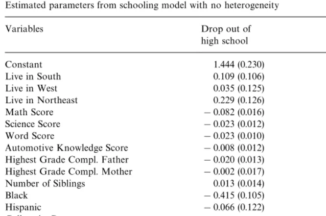
Table 1
Estimated parameters from schooling model with no heterogeneity
Variables Drop out of Attend college
high school
Constant 1.444 (0.230) !1.412 (0.268)
Live in South 0.109 (0.106) 0.387 (0.095)
Live in West 0.035 (0.125) 0.399 (0.109)
Live in Northeast 0.229 (0.126) !0.181 (0.118)
Math Score !0.082 (0.016) 0.074 (0.008)
Science Score !0.023 (0.012) 0.011 (0.012)
Word Score !0.023 (0.010) 0.046 (0.008)
Automotive Knowledge Score !0.008 (0.012) !0.048 (0.009) Highest Grade Compl. Father !0.020 (0.013) 0.040 (0.013) Highest Grade Compl. Mother !0.002 (0.017) 0.039 (0.017)
Number of Siblings 0.013 (0.014) !0.021 (0.015)
Black !0.415 (0.105) !0.324 (0.101)
Hispanic !0.066 (0.122) 0.398 (0.117)
College in County 0.363 (0.102)
Average Wage in County 0.024 (0.071) 0.230 (0.072) Wage in County at Time 0.039 (0.081) !0.235 (0.080)
Cohort Dummies Yes Yes
Standard error ofe
b 0.330 (0.328)
Note: Standard errors in parentheses.
10In order to avoid endogeneity associated with moving, both the local wages and the college in county are measured based on where the respondent lived at age 17.
11I approximatedG(X
bDX1) by assuming that the log deviation of the local labor market variable from its long run mean follows an AR(1) with a gaussian error term. This approximation seems to"t the data well.
long-run mean wage in the county over an approximately thirty-year period. The level of average wages at age 16 enters the decision about whether to drop out of high school and the level of average wages at age 18 enters the decision about whether to attend college.10These variables have the expected signs in the college decision.11Students from counties with higher average income are more likely to attend college, and college attendance is counter-cyclical. Unfortunate-ly, the local labor market variables are much weaker in the high school drop out decision. It is also notable that the standard error ofe
bis not signi"cant in this
model. Looking at the probabilities above we see that this parameter is essen-tially the coe$cient on
PC
UA
X@bbb pb
BA
X@
bbb p
b
B
#/
A
X@bb pb
BD
dG(X
12At essentially every level ofK
1 I found no evidence thatK2should be higher than zero. in a probit for whether the individual drops out of high school. The exclusion restriction that identi"es this parameter is the &college in county' dummy variable. A reduced form probit on high school drop out gives a very similar result, the coe$cient on this variable is positive but not signi"cant. There are a number of di!erent interpretations of this result that the option value of college does not seem to a!ect high school completion. The "rst is that we simply need more data to get a better estimate of the e!ect. A second is that this is evidence that high school students are not forward looking. A third is that the option of college has no value to high school dropouts. That is, it is possible that individuals at the margin of whether to drop out of high school, would not attend college if they did complete high school. For them, the cost of college is irrelevant so the decision about whether to drop out of high school will not be in#uenced by college costs. Distinguishing between these three possibilities is beyond the scope of this paper.
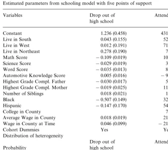
I next present results from the speci"cation in which I allow heterogeneity to enter the model #exibly. The basic strategy is to add points of support to the distribution of the heterogeneity until the likelihood fails to increase by some prespeci"ed amount. In particular, I use the Akaike Information Criterion to choose the number of points of support. The "nal model gave me a value of
K
1"5 andK2"0.12The results of this model are presented in Table 2. There are a few strange aspects to the results. The most striking is the size of the coe$cients and the support points for the heterogeneity distribution in the college attendance decision. With these estimates, the variance ofl
bis very large relative
to the variance ofg
b.gb is essentially irrelevant as a predictor of college
attend-ance. If the variance ofgbwere zero, the model would not be di!erentiable and the standard method of approximating standard errors would not work. While this is not precisely true here, with these estimates it is approximately true so the estimates of the standard errors are not likely to be reliable. Most coe$cients in the schooling decision have the expected signs, but nothing is close to being statistically signi"cant at conventional levels. We also see that the standard error ofe
bonce again is insigni"cant and in this case has the wrong sign. Given the large
and unreliable standard errors it is di$cult to make strong claims about the interpretation of these results. To be able to estimate the dynamics of high school completion, more work needs to be done with hopefully more powerful exclusion restrictions, though"nding such covariates may be very di$cult.
6. Summary and conclusions
Table 2
Estimated parameters from schooling model with"ve points of support
Variables Drop out of Attend college
high school
Constant 1.236 (0.458) 4313.610 (10452.171)
Live in South 0.043 (0.155) 524.178 (3466.992)
Live in West 0.012 (0.191) 715.894 (4722.897)
Live in Northeast 0.278 (0.190) 78.88 (4339.117)
Math Score !0.109 (0.019) 105.399 (272.429)
Science Score !0.029 (0.019) 31.834 (382.258)
Word Score !0.035 (0.013) 85.417 (267.042)
Automotive Knowledge Score 0.005 (0.016) !99.152.942 (312.035) Highest Grade Compl. Father !0.030 (0.017) 59.370 (309.565) Highest Grade Compl. Mother !0.019 (0.025) 111.596 (432.254) Number of Siblings 0.018 (0.021) 12.135 (416.229)
Black !0.507 (0.149) 321.498 (2636.381)
Hispanic !0.147 (0.170) 547.318 (2912.296)
College in County 79.928 (3219.761)
Average Wage in County 0.018 (0.019) 218.244 (1875.892) Wage in County at Time 0.046 (0.099) !216.574 (2091.232)
Cohort Dummies Yes Yes
Distribution of heterogeneity
Drop out of Attend college
Probability high school
0.317 (174.143) 0.000 0.00
0.392 (142.507) 0.000 1728.09
0.166 (25.754) !0.315 3857.79
0.069 (4.681) 392.307 3234.37
0.056 (1.120) 392.700 !2599.65
Standard error ofeb !0.00008 (0.000020)
Note: Standard errors in parentheses.
observables, has no in#uence on the decision. While the model presented here is special, generalizing these results to more complicated "nite time models is straight forward.
I estimate a schooling version of the model in which students "rst decide whether to graduate from high school and then decide whether to attend college. This procedure has only limited success. The model does not show signs of forward looking behavior and reliable standard errors could not be obtained. Part of the problem may be that the exclusion restrictions are weaker than one may hope, and they do not have large support. One possible direction for future research on dynamic schooling models is to obtain more powerful exclusion restrictions which may solve the problems, although this may prove di$cult. More generally this paper has suggested that certain types of exclusion restric-tions with strong support condirestric-tions should help solve the dynamic selection problem. This should be a useful input for empiricists who face this problem.
Acknowledgements
I would like to thank Steve Cameron, Tim Conley, Bo HonoreH, Joe Hotz, Hide Ichimura, Rosa Matzkin, Chuck Manski, Ariel Pakes, several referees, and especially James Heckman for helpful comments. An earlier version of this work was part of my dissertation at the University of Chicago. I gratefully acknow-ledge the "nancial support of the Searle Foundation and the Alfred P. Sloan Foundation. All remaining errors are my own.
Appendix
Proof of Theorem 1. Since every probability I consider in this section conditions
onXandW
2, for the sake of exposition I leave this conditioning implicit. Suppose that there exists (g
a,gb)O(gHa, gHb),e(u) andeH(u) such that for almost
all (x
1,xa,xb),
Pr [g
a(xa)#ea'<ac(x1,e1)]"Pr [gHa(xa)#eHa'<Hac(x1, eH1)] (A.1) and
Pr [g
a(xa)#ea)<ac(x1,e1),gb(xb)#eb'0]
"Pr [gH
a(xa)#eHa)<Hac(x1, eH1),gHb(xb)#eHb'0]. (A.2) I will "rst show thatgHb must be a monotonic transformation of g
b on the
Suppose not, suppose there existX1
b andXbb with positive measure such that
for allx1
b3X1b and allx2b3X2b,
!S6
eb'gb(x1b)'gb(x2b)'!S-eb
gHb(x1
b)(gHb(x2b),
then for d small enough, from the conditions on the support e
b either for
x1
b3X1b,
Pr [g
b(x1b)#eb'0]!Pr [gHb(x1b)#eHb'0]'d,
or forx2
b3X2b,
Pr [gH
b(x2b)#eHb'0]!Pr [gb(x2b)#eb'0]'d.
Without loss of generality suppose it is the"rst. From Condition G1 we can
"nd aX
a(x1b) such that,
Pr [g
a(Xa(x1b))#ea'0](d. Then for allx1b3X1b, d'Pr [g
a(Xa(x1b))#ea'0]
*Pr[g
a(Xa(x1b))#ea'<ac(x1, e1),gb(x1b)#eb'0] (A.3)
"Pr [g
b(x1b)#eb'0]!Pr [gb(xb)#eb'0,ga(Xa(x1b))
#e
a)<ac(x1, e1)]
*Pr [g
b(x1b)#eb'0]!Pr [gb(xb)#eb'0,ga(Xa(x1b))
#e
a)<ac(x1, e1)]
![Pr [gHb(x1b)#eH
b'0]!Pr [gHb(Xb)#eHb'0,gHa(Xa(x1b))
#eH
a)<Hac(x1, eH1)]]
"Pr [g
b(x1b)#eb'0]!Pr [gHb(x1b)#eHb'0]. (A.4)
which is a contradiction sog
bmust be identi"ed to a monotonic transformation
on the limited support.
Now in a similar manner suppose thatg
ais not identi"ed up to a monotonic
transformation. From the same argument as above, there must exist a setX1
a of
positive measure such that for allX1a3X1
a,!S6eb'gb(x1a)'!S-eb and
Pr [g
For anyx
I will now show that I can choosex
1to set the"nal expression arbitrarily close to zero which leads to a contradiction.
Using Condition G3, by dominated convergence it is easy to show that for alle1,
a3X1a we can then construct a sequence of random
variables whose distribution is equivalent to the conditional distribution of (max(g
b(Xb)#eb, 0)D e1,x1,j) for a sequence of x1,j3X1(xa,yj,cj) where as
jPR, y
jB!S6eb and cjP1. Applying the dominated convergence theorem to this sequence, one can show that E(max(g
b(Xb)#eb, 0)D e1,x1j)P0. Thus
we can"nd ajlarge enough such that forx
13X1(xa,yj,cj) we obtain a
contra-diction. h
Proof of Lemma 1. By Assumption G4 we know thatg
a and gb are identi"ed.
Suppose that the lemma were false. Suppose that there exists a random vector (eH
a, eHb) whose distribution cannot be distinguished from that of the true random
vector (e but without loss of generality for some d'0, since the joint distribution of (e
a, eb) is di!erent from the joint distribution of (eHa, eHb), there must be a set of
(g
a,gb) with positive measure such that,
Pr (eH
But then for all members of this set and all x
13supp(X1) for which
g
a"ga(Xa(x1)),
d(Pr (eH
a)!ga,!eHb(gb)!Pr (ea)!ga,!eb(gb)
"Pr [g
a#eHa)0,gb#eHb'0]!Pr [ga#eHa)<ac(x1, eH1),gb#eHb'0]
!(Pr [g
a#ea)0,gb#eb'0]!Pr [ga#ea)<ac(x1,e1),gb#eb'0])
)Pr [g
a#ea)<ac(x1, e1),gb#eb'0]!Pr [ga#ea)0,gb#eb'0]
"Pr [<
ac(x1, e1)*ga#ea'0,gb#eb'0]
)Pr [<
ac(x1, e1)*ga#ea'0].
Following exactly the last part of the proof of Theorem 1, I can show that there exists a set ofX
1 with positive measure such that forx1 in this set, Pr [<
ac(x1, e1)*ga#ea'0](d.
but this is a contradiction, so the result must hold. h
Proof of Theorem 2. This follows trivially from Theorem 1 and Lemma 1 since
the only unobservables in this case areea andeb. h
Proof of Theorem 3. I"rst show that the joint distribution of (e
a!lb,lb#gb) is
identi"ed and then use this fact to show that both the distribution ofg
band that
the joint distribution of (e
a, lb) are identi"ed.
To see that the distribution of (e
a!lb, lb#gb) is identi"ed, recall that we
normalized<
c"0. This was arbitrary, we could have normalized<b"0. We
can basically do that by rede"ning the model in the following manner:
g8a(X
a)"ga(Xa)!E(gb(Xb)DX1), g8a(Xa)"ga(Xa)!E(gb(Xb)DX1), (A.7)
g8
c(Xc)"!gb(Xb),
g8
c(Xc)"!gb(Xb), (A.8)
g8
b(Xa)"0,
g8b(X
a)"0. (A.9)
I now use the characteristic functions of these variables to complete the proof. I will make use of the notation /
Y to denote the characteristic function of
random variable > and /
Y1Y2 to denote the characteristic function of the
random vector (>
1,>2).
Suppose that there exist random variables (eH
a, gHb,lHb) that generate the same
I can now show that the joint distribution ofl
bandeais identi"ed sincegbis
independent of them and has a known distribution.
/
The characteristic function and thus the distribution of (e
a,la) is identi"ed and
the full distribution of the unobservables is known. h
References
Aakvik, A., Heckman, J., Vytlacil, E., 1999. Local instrumental variables and latent variable models for estimating treatment e!ects. Unpublished manuscript, University of Chicago.
Altonji, J., 1993. The demand for and return to education when education outcomes are uncertain. Journal of Labor Economics 11, 48}83.
Belzil, C., Hansen, J., 1997. Estimating the returns to education from a non-stationary dynamic programming model. Centre for Labour Market and Social Research Working Paper No. 97-06. Buchinsky, M., Leslie, P., 1996. A dynamic model of education choices in the United States: learning
from a cross-section. Unpublished manuscript, Brown University.
Cameron, S., Taber, C., 1994. Assessing nonparametric maximum likelihood models of dynamic discrete choice. Unpublished manuscript.
Cameron, S., Taber, C., 1998. Borrowing constraints and the returns to schooling. Unpublished manuscript, Northwestern University.
Card, D., 1998. The causal e!ect of education on earnings. Center for Labor Economics, University of California at Berkeley Working Paper No. 2.
Chamberlain, G., 1986. Asymptotic e$ciency in semi-parametric models with censoring. Journal of Econometrics 32, 189}218.
Comay, Y., Melnik, A., Pollatschek, M., 1973. The option value of education and the optimal path for investment in human capital. International Economic Review 14, 421}434.
Cosslett, S., 1983. Distribution-free maximum likelihood estimator of the binary choice model. Econometrica 51, 765}782.
Eckstein, Z., Wolpin, K., 1989. The speci"cation and estimation of dynamic stochastic discrete choice models. Journal of Human Resources 24, 562}598.
Eckstein, Z., Wolpin, K., 1997. Youth employment and academic performance in high school. Unpublished manuscript, University of Pennsylvania.
Flinn, C., Heckman, J., 1982. New methods for analyzing structural models of labor force dynamics. Journal of Econometrics 18, 115}168.
Heckman, J., 1990. Varieties of selection bias. American Economic Review 80, 313}318.
Heckman, J., HonoreH, B., 1990. The empirical content of the Roy model. Econometrica 58, 1121}1149.
Heckman, J., Singer, B., 1984. A method for minimizing the impact of distributional assumptions in economic models for duration data. Econometrica 52, 271}320.
Heckman, J., Vytlacil, E., 1999. Local instrumental variables and latent variable models for identifying and bounding treatment e!ects. Unpublished manuscript, University of Chicago. Hotz, V.J., Miller, R., 1993. Conditional choice probabilities and the estimation of dynamic models.
Review of Economic Studies 60, 497}529.
Ichimura, H., Taber, C., 1999. Estimation of treatment e!ect counter factuals under limited support conditions. Unpublished manuscript, Northwestern University.
Keane, M., Wolpin, K., 1997. The career decisions of young men. Journal of Political Economy 105, 473}522.
Manski, C., 1975. Maximum score estimation of the stochastic utility model of choice. Journal of Econometrics 3, 205}228.
Manski, C., 1988. Identi"cation of binary response models. Journal of the American Statistical Association 83, 729}738.
Matzkin, R., 1990. Least concavity and the distribution-free estimation of nonparametric concave functions. Unpublished manuscript.
Matzkin, R., 1992. Nonparametric and distribution-free estimation of the binary threshold crossing and the binary choice models. Econometrica 60, 239}270.
Matzkin, R., 1993. Nonparametric identi"cation and estimation of polychotomous choice models. Journal of Econometrics 58, 137}168.
Pakes, A., 1986. Patents as options: some estimates of the value of holding European patent stocks. Econometrica 54, 755}784.
Pakes, A., Simpson, M., 1989. Patent renewal data. In: Bailey, Winston (Eds.), Brookings Papers on Economic Activity. The Brookings Institute, Washington.
Roy, A.D., 1951. Some thoughts on the distribution of earnings. Oxford Economic Papers (New Series) 3, 135}146.
Rust, J., 1987. Optimal replacement of GMC bus engines: an empirical model of Harold zurcher. Econometrica 55, 999}1035.
Taber, C., 1996. Semiparametric identi"cation and heterogeneity in discrete choice dynamic pro-gramming models. Unpublished manuscript, Northwestern University.
Taber, C., 1998. The rising college premium in the eighties: return to college or return to ability? Unpublished manuscript.
Thompson, T.S., 1989. Identi"cation of semiparametric discrete choice models. Unpublished manu-script.
Weisbrod, B., 1962. Education and investment in human capital. Journal of Political Economy 70, 106}123.