Control by a magnetic field of the instability of a Hadley circulation in
a low-Prandtl-number fluid
L. Davousta, R. Moreaub,*, R. Bolcatob
aLEGI, Domaine universitaire, ENSHMG BP95, 38042 Grenoble cedex, France bMADYLAM, Domaine universitaire, BP 95, 38402 St Martin d’Hères cedex, France
(Received 30 April 1998; revised 20 October 1998; accepted 30 November 1998)
Abstract– The Hadley circulation of a low-Prandtl-number fluid (mercury) is driven by a horizontal temperature gradient within a horizontal differentially-heated cylinder of very small aspect-ratio(radius/length=ε=0.05). Transition to turbulence, investigated within the core region of this internal buoyancy-driven recirculating flow, is controlled by imposing a smoothly decreasing or increasing magnetic fieldB0(vertically applied and
permanent).
For a moderate Grashoff number,Gr1T∼105, the transition turns out to be well-characterised by time-dependent temperature oscillations. A first sub-critical bifurcation gives rise simultaneously to two waves which exhibit the same frequencyf1; and the flow experiences a stronger and stronger
non-linear coupling between temperature and velocity fields. The first wave, transversal, is detected in the central cross-sections of the core flow along the horizontalY-axis parallel to the differentially heated side walls, whereas the second wave, a 3-D longitudinal wave, is travelling along the axis of the cylindrical enclosure. As the magnetic field still decreases, the amplitude of the transversal wave grows and, subsequently, the spectral content of the 3-D longitudinal wave is consistently modified. With a still decreasingB0a Hopf supercritical bifurcation, whose control parameter is found to be
a modified Rayleigh numberRaG, is detected before the introduction of a chaotic regime; this bifurcation yields a 3-D longitudinal standing wave of a low frequencyf2.
For a larger Grashoff number, Gr1T ∼106, the transition is complicated by the occurrence of some stabilisation windows even after a first destabilisation of the core flow or by the occurrence of some oscillatory windows even after a first stabilisation.Elsevier, Paris
magnetic field / oscillations / stability / bifurcation
1. Introduction
During the last two decades, an abundant number of theoretical, numerical (Busse and Clever [1] and Clever and Busse [2]) and experimental investigations (Libchaber et al. [3] and Koster [4]) have been devoted to the Rayleigh–Bénard (R–B) convection of low-Prandtl-number fluids. As well as the first bifurcation which yields steady 2-D rolls (supporting flow), the following bifurcations are responsible for a noticeable diversity of new hydrodynamical time-dependent regimes. With the R–B configuration, it is necessary to increase the applied vertical temperature gradient beyond a critical value in order to enhance 2-D rolls. This need to destabilise the fluid initially at rest is obviously due to the fact that only a temperature gradient which is not aligned with gravity is able to drive a buoyancy-driven cell. Practically, the limited dimensions of the geometry often cause the wave number related to the 2-D rolls to be frozen beyond a threshold. As a consequence, this ‘basic’ flow, which nevertheless results from a first bifurcation, allows for analysis of the roads encountered to a temporal chaos.
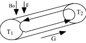
As far as the so-called Hadley circulation is concerned, a thermogravitationnal flow is driven by a horizontally applied temperature gradient whose vector product with gravity is hence not curl-free. The
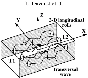
Figure 1.A sketch of 3-D longitudinal oscillatory rolls.
subsequent buoyancy torque makes this truly basic recirculating flow to be upwards in the hot region and downwards in the cold region. Subsequently, as well as the R–B configuration, the Hadley configuration may fairly be thought of as a practical support for investigators of the roads to chaos. As a matter of fact, this configuration is also relevant to the horizontal Bridgman crystal growth technique. In the case of the Bridgman solidification, it is well-known that time-dependent oscillations within the melt and also near the solidification interface cause the semiconductor crystal to solidify, to remelt, and so forth, yielding unwelcome striations (Langlois [5]). Since pioneering work by Hart [6], many theoretical and numerical studies have been devoted to the linear and non-linear stability analysis of the Hadley flow of low-Prandtl fluids in 2-D or 3-D enclosures. These include e.g. the work by Gill [7], Hart [8], Roux et al. [9], Henry and Buffat [10], Ben Hadid and Roux [11]. All authors agree to predict some inherently 3-D longitudinal oscillatory rolls and steady transversal 2-D rolls. These modes have the typical form,A(Z)exp[i(kxX+kyY )+αt], where symbols kx,ky, α and
A(Z) denote, respectively, theX- and Y-components of the wave vector, the eigenvalue and the amplitude assumed to depend only onZ. To illustrate this, a set of three 3-D longitudinal oscillatory rolls, whose axis are perpendicular to the heated side walls, are sketched infigure 1. These parallel rolls yield a 2-D oscillatory transversal wave. For the sake of clarity, the Hadley circulation has not been sketched. Pratte and Hart’s [12] and Braunsfurth and Mullin’s [13] works are the few experiments performed on (parallelepipedic) cavities filled with, respectively, mercury and gallium. Both of them concentrate on the nature of the bifurcations involved during destabilisation of the core flow when varying three non-dimensional numbers in a systematic way, namely:
– the aspect ratio,ε, defined as the ratio between the typical transversal lengthR0, and the axial lengthL,
– the Prandtl number, defined as Pr =ν/α, which relates the momentum diffusivity ν to the thermal diffusivityα,
– the Grashoff number Gr1T, proportional to the temperature difference 1T applied between the two
side walls of the enclosure, is defined as Gr1T =(gβ1T R04)/(Lν2). The symbols β and g denote the
volumetric expansion and gravity.
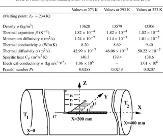
Figure 2.Configuration under study.
Hartmann numberHa, here defined asHa=(σ/ρν)1/2B
0R0, whereσandρdenote, respectively, the electrical
conductivity and the density of the involved fluid. McKell et al. [17] also analysed some time-dependent regimes encountered after destabilisation. However, there still remains a lack of understanding on the nature of these oscillations. Moreover, no spectral description of the transition is available yet. It is then one of the aims of this paper to complement the former studies in order to provide both mechanical and spectral descriptions of this transition in terms, respectively, of waves and power spectral densities (PSD). We now focus on the core region of a particular HIMF which stands within a horizontally extended cylinder (ε=0.05,figure 2).
2. Brief statement of the laminar core flow
Compared with any other orientation, the vertical uniform magnetic field yields the most efficient damping of the flow since the Hartmann layer, which develops along the longitudinal cylindrical wall, stays electrically inactive (Alboussière et al. [18,19]). As a matter of fact, as soon as Ha is of the order of 10, the flow is laminar and the effective viscosity is reduced to the molecular level (Davoust et al. [20]). After previous theoretical, numerical and experimental developments (Cowley [21], Davoust et al. [20,22]), the laminar core flow is well-known and understood. This stands as a fully-developed shear flow, axially directed, on which are superimposed four additional vortices localised symmetrically within the four quadrants of the central cross-sections of the cylinder. Though important in the end regions, inertia cannot play a key role here since the aspect ratioε of the cylindrical cell is much smaller than unity. Therefore, the core flow is controlled by the balance between the curls of buoyancy and Lapace force. This balance yields a typical velocity scale proportional to GrG/Ha2, based on the core temperature gradientG. Similarly toGr1T, the Grashoff numberGrGis written as
GrG=gβGR04/ν2. Non-linear terms in the energy equation are weighted by a new non-dimensional number,
namely a modified Rayleigh number, referred to asRaG, and defined asRaG=Pr·GrG/Ha2(Cowley [21]).
3. Experimental facilities
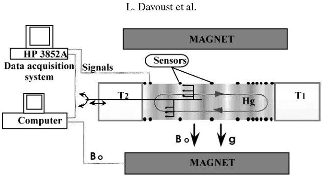
Figure 3.The experimental set-up.
The investigation is performed with an experimental set-up involving a horizontal cylindrical cell of small aspect ratio,ε=0.05 (radiusR0=20 mm, lengthL=400 mm), filled with mercury. The flow is subjected to
a permanent vertical magnetic fieldB0 whose uniformity is stated to be±1.8% in the worst conditions. Two copper disks, located at the two ends of the cell, are cooled or heated using water circulation in passages within them; these passages, in the shape of spirals, are designed in such a way that the direction of the circulation of the water is alternatively inverted. As a consequence, the two end temperaturesT1(cold end wall) andT2(hot
end wall) are controlled with a precision of±0.01 K by the way of commercial temperature regulators. The
cylindrical longitudinal wall, made of glass, is surrounded by a thick copper wall and by a thermally insulating coating. Such a device allows adiabaticity and as a consequence, uniformity of the horizontal temperature gradient is achieved with a precision better than±1%. The experimental cell is equipped with 55 thermocouples
(distributed along eleven half-circles) which do not protrude into the flow. These thermocouples are classically built with chromel and constantan wires whose the two separated heads (diameter 100µm) are set close to each other at the wall, skimming the mercury surface. These 55 thermocouples, whose cold welded joints are all gathered in a cold box (temperatureT0 controlled at±0.01 K), are characterised by a weak time response
(less than 0.1 s) because of a small contact surface: mercury, which is of course locally in contact with the heads of the constantan and chromel wires, plays the role of the second welded joint. Just before a 13 bits A/D conversion, the measured Seebeck signal is sent to a linear amplifier with a gain of about 1950 and a high-pass filter (cut-frequency of 0.001 Hz). To investigate the time-dependence of the flow, a computer both records the temperature signals by the way of a HP3852A data acquisition system (figure 3) and, simultaneously, pilots step by step the increase or decrease of the Ha number. Many trials have been done decreasing either the value of the step onHaor extending the associated time delays. Indeed, it is crucial to be sure that quasi-steady conditions are well-achieved during the phases of stabilisation or destabilisation. Finally, a step of the Hartmann number,δHa=0.021, related to a time delay of 10 s is a good compromise. Such a procedure guarantees a
sufficient reproducibility on the onset of the oscillations. When characterising the transition at a low Grashoff number (Section 5 of this paper), acquisition of the signals was also performed every timeHawas increased or decreased by an incremental value of 0.1. There was a delay of one hour before each of these acquisitions. Such a precaution allows us to identify without any doubt the nature of the involved bifurcations during the transition.
the hot end wall to the centre of the cell in such a way that characterisation of the temperature oscillations is performed. A close inspection was devoted to ascertaining that no significant electric or mechanical perturbations of the flow were encountered (typical velocity of the order of 0.001 to 0.01 m/s).
– As a matter of fact, since the second rank of thermocouples (t4tot7) is capable of moving freely behind
the first rank (t1tot3), the authors did many trials to check that no vortex street is promoted downstream
of the first rank.
– The electric current lines within the fluid close themselves along circles within any cross-section of the core flow. Hence, these electric paths, by surrounding the main support of the movable probe (electrically insulating), cannot be significantly disturbed (Davoust et al. [22]).
– Finally, the quite gentle course ofB0 (a step of 0.5 Gauss every 10 s) protects the experiment from any
additional induced electric fields (unsteady term of the Ohm’s law) in the experiments.
Turning now to the control parameters of our experiments, namely the Grashoff and the Hartmann numbers, at a low level of convection (Gr1T ∼104–105), the internal probe is found to be more sensitive than the
wall-thermocouples to the onset of temperature oscillations arising from the background noise (when Ha is decreasing). Among the explanations which come to mind, one is related to the internal movable probe, protruding within the mercury flow, and which might artificially modify thresholds. A second is due to diffusion through the thermal boundary layer (thicknessR0/RaG) which develops along the longitudinal wall of the cell;
diffusion may decrease the sensibility of the 55 wall-thermocouples. To investigate this question, experiments driving and damping the oscillatory instabilities were conducted at a high level of convection (Gr1T ∼5×10⁵
and more) so that the wall-thermocouples, as well as the thermocouples attached to the internal movable probe were able to deliver the same thresholds for the oscillatory signals. Then, two cases were examined:
– first, the internal movable probe was introduced within the melt,
– and second, for the sake of comparison, the internal movable probe was pulled out of the core flow, against the hot end wall.
For these two cases, the critical Hartmann numbers delivered by all the thermocouples, included the non-protruding wall-thermocouples, were found to be the same. As a consequence, we think the second explanation (diffusion through the thermal boundary layer) is the correct one. We thus believe that the results given hereafter, are indicative of both the onset and the nature of the thermal oscillations that would occur if no internal probe were present within mercury. On the other hand, the thresholds are dramatically sensitive to any electrical connection from a point of the fluid domain to ground. Since one of our aims was to give a benchmark for any further direct numerical simulations, which may also provide a dynamical insight in the mechanisms responsible for the onset of oscillatory instabilities, all the experiments were always performed when no point of the fluid domain was connected to ground.
4. Transition: global features
At a moderate value of the applied Grashoff number,Gr1T lower than 9×10⁵, destabilisation of the laminar
core flow occurs when the Hartmann number reduces to a critical value, here referred to asHa∗
1. Then,
Figure 4.Stability diagram for the temperature oscillations (in the planeGr1T−Ha).
The first region, the region A, is associated to a moderate range of the Grashoff number and is characterised by the hysterisis mentioned earlier. The critical Hartmann numberHa∗2for which the oscillations are damped, is found to follow the scaling lawHa∗
2∼(Gr1T)1/2.
The second region, here referred to as region B, relates to higher values of the Grashoff number,Gr1T ∼106
and above, and exhibits few stabilisation and oscillatory windows. The oscillatory windows are defined as windows which arise paradoxically after a first stabilisation of the oscillatory regime at Ha∗
2. Inside these
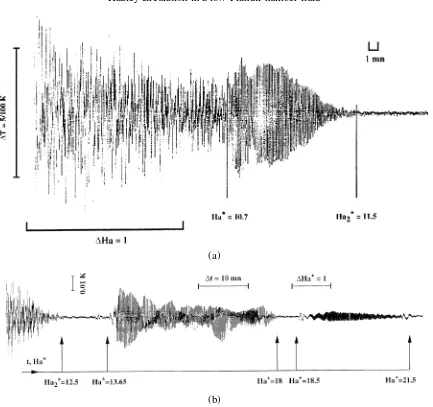
oscillatory windows which also occur before a definitive stabilisation of the unsteady core flow, time-dependent temperature oscillations are thus in place: infigure 5(b), an oscillatory window is for example detected between two increasing values of the Hartmann numberHa∗ (gap 13.65–18). Increasing the Hartmann number a little more up to higher values, here referred to asHa∗, again one and indeed two oscillatory windows can be made evident (figure 5(b), gaps 13.65–18 and 18.5–21.5). A final stabilisation is achieved only whenHareaches the threshold Ha2(Ha2>Ha∗2,figure 5(b)). And conversely, when decreasing Ha, the stabilisation windows are
observed to occur after a first oscillatory regime. Then, the Hartmann numberHa, which is already lower than Ha∗
1, has to decrease to an other thresholdHa1(Ha1<Ha∗1) which yields the oscillating regime definitively.
Any dependence on time of the presence of these oscillatory/stabilisation windows has to be ruled out. In other words, since those windows are quite stable in time, the key feature of the transition here seems to be the fact that any intermittent pattern has disappear. However, on the other hand, the occurrence of the windows is found to depend on the axial position within the cell. As soon as the Hartmann number is larger thanHa∗
2, stabilisation of the former temperature oscillations, though observed at the center of the cell, is no
longer diagnosed at other locations. At a fixed value of the Hartmann number Ha∗, Ha∗ being larger than Ha∗
2, some oscillatory windows may also be detected moving the sensors to other axial locations within the
vertical longitudinal mid-planeXZ. Finally, in region B, we think there is an actual difficulty in characterising the transition.
(a)
(b)
Figure 5.Damping of the temperature oscillations within the core flow in an increasing magnetic field. (a)Gr∼8.38×10⁵(X=200 mm,α=90◦);
(b)Gr∼1.13×10⁶(X=300 mm,α=90◦).
control parameter of the transition. As an example, a relative variation of 10–20% onPr is able to promote bifurcations in gallium (see the experimental work by Braunsfurth and Mullin [13]). A close inspection of the thermophysical characteristics of mercury as a function of the temperature (table I) makes this explanation consistent, since the mean core temperature,T1+1T /2, takes values between 289 K and 304.5 K(T1=288 K,
T2=290−320 K,1T =T2−T1).
5. Transition in region A at a moderate Grashoff numberGr1T =2.62×10⁵
Table I.Thermophysical characteristics of mercury (from Eckert and Drake [24]).
Values at 273 K Values at 293 K Values at 323 K (Melting point:TF=234 K)
Figure 6.Sensors locations in the middle cross-section(X=200 mm).
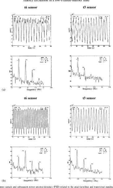
waves, all the temperature signals which are now exhibited are recorded from thermocouples located at fixed positions within the central cross-section (figure 6). The first rank (thermocouples t1 to t3) is located at the
angular positionα=0◦, whereas the second one (thermocouplest4tot7) is inclined atα=90◦.
5.1. Characterisation of the transition in terms of waves
As mentioned earlier, whenHa reduces to the value Ha∗
1, we observe a primary bifurcation which makes
the core flow go from a laminar to an oscillatory regime; this bifurcation #I gives simultaneously rise to two waves of the same frequency(f1=43±0.5 mHz). As the first one is travelling along the axis of the cell (wave
lengthλX∼60±5 mm) within the vertical longitudinal mid-plane XZ (figure 7(a), T6 sensor), the other is
detected within the vertical transversal mid-planeYZ (figure 7(a), T3sensor). This latter transversal standing
wave, whose wave lengthλY is of the order of the diameter, oscillates in opposition of phase with respect to
XZ mid-plane (antisymmetric character). When we further decreaseHa, the wave amplitude grows. Because of a stronger and stronger non-linear coupling between the temperature and velocity fields asRaG increases
(RaG∼1/Ha2), the temperature oscillation detected within the vertical longitudinal mid-planeXZand initially
only related to the former 3-D axial travelling wave, is now more and more enriched with harmonics foils. This is shown on power spectral densities (PSD) where the fundamental peak at frequency f1 (figure 7(a),
t6sensor) becomes smaller than its first harmonic peak at frequency 2f1(figure 7(b),t6sensor). Regarding our
experimental results, the 2-D transversal wave may be thought of as evidence of a horizontal oscillatory motion of a 3-D longitudinal roll (Bojarevics [25]).
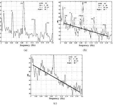
Then, decreasing againHa down toHa∗∗1 , a third wave of a much smaller frequency(f2=9±0.5 mHz),
(a)
(b)
Figure 7.Temperature signals and subsequent power spectral densities (PSD) related to the axial travelling and transversal standing waves. (a)Ha=
Figure 8.Time modulation for the axial standing wave (Ha=2.35, t6sensor).
(a) (b)
(c)
(a) (b) (c)
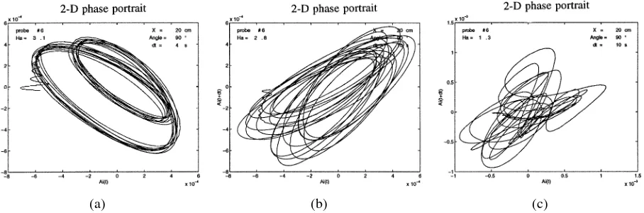
Figure 10.Two-dimensional projections of the reconstructed phase portraits for thet6temperature signal. (a)Ha=3.11; (b)Ha=2.82; (c)Ha=1.28.
(figures 8and 9(a)). Far from theXZ mid-plane, the amplitude of this third wave (clearly detected by thet6
sensor) quickly decreases; there is no evidence of af2-frequency modulation ont2ort3temperature signals.
Then, as Hacontinues to decrease (Ha<Ha∗∗1 ), the mean negative slope of the power spectral densities (PSD) is observed to be steeper and steeper (figures 9(a)–9(c), PSD are plotted in semi-log scales). This means that the level of spectral energy is growing as a chaotic regime arises progressively.
This very classical scenario may also be observed by the way of phase portraits (figures 10(a)–10(c)) reconstructed from thet6 temperature signals. Following Swinney [26], it is easy to check that the structure
of these phase portraits does not change whether an extra dimension is added (from a 2-D to a 3-D plot). As a consequence, the 2-D projections of the reconstructed phase portraits are plotted onfigures 10(a)–10(c). Topology of the reconstructed phase portrait onfigure 10(a) is equivalent to the one of a circle (T1-torus), in fair agreement with a mono-periodic regime already active atHa=3.11 (single frequencyf1). The presence of
a strong harmonic foil on the temperature signal (figure 7(b),t6sensor) makes this phase portrait to possess two
loops.Figures 10(b)and10(c)suggest that chaos is achieved from the break-up of a bi-periodic regime based on the frequencies f1 and f2. The continuous series of points displayed from a Poincaré map realised from
the phase portrait plot onfigure 10(b)(Ha=2.82) would suggest the presence of a quasi-periodic sequence
rather than a frequency-locked one. Nevertheless, a more elaborate study of this scenario both by way of data acquisitions of very long time duration and the systematical use of Poincaré maps is not the aim of this paper.
5.2. Characterisation of the transition in terms of bifurcations
Now, when we increase the Hartmann number, chaos disappears and the subsequent oscillatory temperature signals exhibit again the basic frequenciesf1andf2. As Ha reaches the critical valueHa∗∗1 , oscillatory signals
are again characterised by the single frequencyf1. As there is no sign of hysterisis for the bifurcation #II and
since the frequencyf2remains constant for supercritical values ofHa, a Hopf supercritical bifurcation may be
expected at the onset of the axial standing wave (the third wave). As frequencyf2is much smaller thanf1, it is
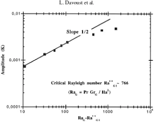
also possible to measure accurately the amplitude of the oscillation associated to this third wave. As a matter of fact, the modified Rayleigh numberRaGis found to be the actual control parameter of the bifurcation #II: close
to the bifurcation, the amplitude is seen to scale linearly with the square root of the gapRaG−Ra∗∗G1 (figure 11).
Figure 11.Amplitude of the modulation due to the axial standing wave versus the differenceRaG−Ra∗∗G1.
Inside very small or large aspect-ratio containers, it has been demonstrated from the R–B configuration that 2-D rolls usually experience either successive nucleations and dislocations or a slow aperiodic drift motion. Such phenomena lead to a weak time-modulation of the temperature signals and to a subsequent increasing level of intrinsic noise (Ahlers et al. [27], Manneville [28,29]). Subsequently, such a slow dynamical process is able to induce negative slopes on PSDs far before chaos arises. To interpret the presence of the negative slope observed on our PSD (figures 7(a),7(b), 9(a)), we may infer that because of the axial extension of the cell, some quasi-steady structures are able to move slightly during transition. These quasi-steady structures may stem either from a shear mechanism related to the basic core flow, such as 2-D convective cells distributed along the cylinder (Bojarevics [25]), or from inertial effects enhanced within the recirculating end regions (see Hart [8]). However, such phenomena remain to be investigated. And as a matter of fact, they would lend themselves very well to a direct visualisation by the way of a real-time X-ray radioscopy, as now currently practised by Koster [4].
6. Conclusion
An experimental set-up has been developed in order to reach the following goals: to promote stabilisation or destabilisation of a thermogravitationnal Hadley recirculating flow, free of any Marangoni effects, in a cylinder filled with mercury and submitted to a uniform vertical magnetic fieldB0. Our experiments focus on the core
region of the flow. Whatever the value of the applied Grashoff number,Gr1T, temperature oscillations are found
to occur with reproducibility whenB0is smoothly decreased. Subsequently, an overall stability diagram has
been constructed which gives a benchmark to any future (non-linear) numerical and theoretical developments. At a moderate scale of the Grashoff number, Gr1T ∼105, oscillatory instabilities occur by way of a
subcritical bifurcation which yields two waves, a 3-D longitudinal travelling wave and a transversal standing wave. These two waves of frequency f1 are strongly coupled. If the applied magnetic field (or the Hartmann
is associated to a Hopf supercritical bifurcation whose control parameter is found to be a modified Rayleigh number RaG =Pr·GrG/Ha2 (Cowley [21]). Chaos arises from the breakup of the subsequent bi-periodic
regime based on the frequencies f1 and f2. As far as the negative slopes observed on the power spectral
densities before the onset of chaos are concerned, an increasing number of some steady modes, which are not truly frozen along the axis of the cell, is put forward as a possible explanation.
At a larger scale of the Grashoff number, Gr1T ∼106, the transition is drastically complicated by the
occurrence of some stabilisation and oscillatory windows along the core.
Acknowledgements
The authors thank Prof. H. Ben Hadid and Dr. D. Henry from the LMFA of the École Centrale de Lyon for the development of direct numerical simulations as part of a contract with CNES. Both their comments and the agreement between some of our experimental results and their numerical results reinforce a very nice collaboration. The authors are also indebted to CNES (microgravity division) for its decisive financial support.
References
[1] Busse F.H., Clever R.M., An asymptotic model of two-dimensional convection in the limit of low Prandtl number, J. Fluid Mech. 102 (1981) 75–83.
[2] Clever R.M., Busse F.H., Convection at very low Prandtl number, Phys. Fluids A 2 (1990) 334–339. [3] Libchaber A., Fauve S., Laroche C., Two-parameter study of the routes to chaos, Physica D 7 (1983) 73–84.
[4] Koster J.N., Visualization of Rayleigh-Bénard convection in liquid metals, Eur. J. Mech. B-Fuids 16 (3) (1997) 447–454. [5] Langlois W.E., Buoyancy-driven flows in crystal growth melts, Ann. Rev. Fluid Mech. 17 (1985) 191–215.
[6] Hart J.E., Stability of thin non-rotating Hadley circulations, J.Atmos. Sci. 29 (1972) 687–697. [7] Gill A.E., A theory of thermal ocillations in liquid metals, J. Fluid Mech. 64 (3) (1974) 577–588.
[8] Hart J.E., Low-Prandtl number convection between differentially heated walls, Int. J. Heat Mass Trans. 26 7 (1983) 1069–1083.
[9] Roux B., Ben Hadid H., Laure P., Hydrodynamical regimes in metallic melts subject to a horizontal temperature gradient, Eur. J. Mech. B-Fuids 8 (5) (1989) 375–396.
[10] Henry D., Buffat M., Two and three-dimensional numerical simulations of the transition to oscillatory convection in low-Prandtl number fluids, Prepublication (1990).
[11] Ben Hadid H., Roux B., Buoyancy-driven oscillatory flows in shallow cavities filled with low-Prandtl-number fluids, in: Roux B. (Ed.), Numerical Simulation of Oscillatory Convection in Low-PrFluids, Notes on Numerical Fluid Mechanics, Vol. 27, Vieweg, 1990, pp. 25–34. [12] Pratte J.M., Hart J.E., Endwall driven, low-Prandtl number convection in a shallow rectangular cavity, J. Cryst. Growth 102 (1990) 54–68. [13] Braunsfurth M.G., Mullin T., An experimental study of oscillatory convection in liquid gallium, J. Fluid Mech. 37 (1996) 199–219.
[14] Utech H.P., Flemings M.C., Elimination of solute banding in indium antimonide crystals by growth in a magnetic field, J. Appl. Phys. 37 (5) (1966) 2021–2024.
[15] Chedzey H.A., Hurle D.T.J., Avoidance of growth-striae in semiconductor and metal crystals grown by zone-melting techniques, Nature 5039 (1966) 933–934.
[16] Hurle D.T.J., Jakeman E., Johnson C.P., Convective temperature oscillations in molten gallium, J. Fluid Mech. 64 (1974) 565–576. [17] McKell K.E., Broomhead D.S., Jones R., Hurle D.T.J., Europhys. Lett. 12 (6) (1990) 513–518.
[18] Alboussiere T., Garandet J.-P., Moreau R., Buoyancy-driven convection with a uniform magnetic field, Part I: asymptotic analysis(Ha≫1),
J. Fluid Mech. 253 (1993) 545–560.
[19] Alboussiere T., Garandet J.-P., Moreau R., Asymptotic analysis and symmetry in MHD convection, Phys. Fluids 8 (1996) 2215–2226. [20] Davoust L., Moreau R., Bolcato R., Alboussière T., Neubrand A.-C., Garandet J.P., Influence of a vertical magnetic field on convection in the
horizontal Bridgman crystal growth configuration, Magnetohydrodynamics 31 (3) (1995) 218–227.
[21] Cowley M.D., The effect of a buoyancy-driven magnetohydrodynamic flow on the temperature distribution in a horizontal cylinder, Magnetohydrodynamics 31 (3) (1995) 228–238.
[22] Davoust L., Moreau R., Cowley M.D., Tanguy P.A., Bertrand F., Numerical and analytical modelling of the MHD buoyancy-driven flow in a Bridgman crystal growth configuration, J. Cryst. Growth 180 (1997) 422–432.
[23] Ben Hadid H., Henry D., Unsteady three-dimensional buoyancy-driven convection in cylindrical cavities with and without magnetic field, J. Cryst. Growth 180 (1996) 435–441.
[25] Bojarevics V., Buoyancy driven flow and its stability in a horizontal rectangular channel with an arbitrary oriented transversal magnetic field, Magnetohydrodynamics 31 (3) (1995) 333–343.
[26] Swinney H.L., Observations of order and chaos in non-linear systems, Physica D 7 (1983) 3–15.
[27] Ahlers G., Cannell D.S., Steinberg V., Time-dependence of flow patterns near the convective threshold in a cylindrical container, Phys. Rev. Lett. 54 (13) (1985) 1373–1376.