ANALYSIS
Internal migration and the environmental Kuznets curve for
US hazardous waste sites
Kishore Gawande, Alok K. Bohara, Robert P. Berrens *, Pingo Wang
Department of Economics,Uni6ersity of New Mexico,Albuquerque,NM87131,USA Received 4 June 1999; received in revised form 28 September 1999; accepted 4 October 1999
Abstract
In the recent special issue of Ecological Economics devoted to the environmental Kuznets curve (EKC) hypothesis, Rothman speculates that: ‘‘what appear to be improvements in environmental quality may in reality be indicators of increased ability of consumers in wealthy nations to distance themselves from the environmental degradation associated with their consumption’’ (Rothman, D., 1998. Environmental Kuznets curves – real progress or passing the buck?: a case for consumption-based approaches. Ecol. Econ. 25, 178). Consistent with Rothman’s general hypothesis of ‘distancing’ as a possible source of EKC results, this empirical study advances and tests a line of argument in which internal migration plays a central explanatory role for an observed EKC for US hazardous waste sites. Two specific hypotheses tested are: (i) proximity to hazardous waste site build-up emerges as a factor in the migration decisions of individuals as per capita income increases beyond a threshold level; and (ii) the level of income at which the EKC turns downwards is equal to the threshold level of income in (i). Results provide evidence that migration is a contributing factor to the observed EKC. © 2000 Elsevier Science B.V. All rights reserved.
Keywords:Environmental Kuznets curve; Hazardous waste; Migration
www.elsevier.com/locate/ecolecon
1. Introduction
A recent special issue of Ecological Economics (volume 25, no. 2) was devoted to the environ-mental Kuznets curve (EKC) hypothesis. Since the findings of the inverted-U relationship be-tween a variety of environmental pollutants and per capita income in the cross-country studies by
Shafik and Bandyopadyhay (1992), Grossman and Krueger (1993, 1995), considerable effort has been devoted to investigating the empirical evi-dence for EKCs, and interpreting the policy
rele-vance of these reduced form relationships.1
1Selected EKC studies include: Shafik (1994); Selden and Song (1994) and Holtz-Eakin and Selden (1995). Cavlovic et al. (2000) synthesize results from more than 25 EKC studies using a statistical meta-analysis, and predict income turning points for 11 different pollution categories while controlling for methodological differences across studies.
* Corresponding author. Tel.: +1-505-2779004; fax: + 1-505-2779445.
E-mail address:[email protected] (R.P. Berrens)
Beckerman (1992) interprets EKC results as a kind of general evidence that societies can grow out of any environmental problem. This is in juxtaposition to Arrow et al. (1995) who argue that the EKC has been shown in only select settings, and where present may be due to shiftable negative externalities, may not hold in the future due to ecological thresholds, and should not be interpreted as a substitute for en-vironmental policy or institutional change.
A variety of theoretical models of the EKC are emerging (Selden and Song, 1995; Mc-Connell, 1997). However, our understanding of both the full array of causal mechanisms and the resulting policy implications remains incom-plete. Suggested mechanisms for the
‘de-cou-pling’ between per capita income and
environmental pollution include: changes in the composition of output, changes in production technologies, induced environmental policy re-sponses towards stricter regulation, or some mix (Grossman and Krueger, 1996). In the recent special issue of Ecological Economics, a number of studies make cases for including various ex-planatory variables in EKC studies, such as measures of power (in)equity and social factors (Torras and Boyce, 1998), trade-related measures (Suri and Chapman, 1998), and spatial intensity of economic activity (Kaufmann et al., 1998). Further, Rothman (1998) argues for increased investigation of the relationship between ‘con-sumption based’ environmental indicators (e.g. ‘ecological footprints’) and measures of eco-nomic growth.
Rothman (1998) argues that solving environ-mental problems associated with growth must mean more than ‘passing them off’ to people in other times and places. Rothman (1998) (p. 178) speculates that: ‘‘what appear to be improve-ments in environmental quality may in reality be indicators of increased ability of consumers in wealthy nations to distance themselves from the environmental degradation associated with their
consumption’’. To extend this speculation,
mechanisms for such distancing might include both moving polluting sources (e.g. for flow pol-lutants) as emphasized by Rothman (1998) (p.
186), and selected households moving away from pollution concentrations (e.g. for stock pollutants). The focus of this study is on the latter.
Specifically, the objectives of this empirical study are twofold: (i) to confirm the presence of an EKC relationship for US hazardous waste sites; and (ii) to investigate the potential for in-ternal migration to be a contributing explana-tory factor.
In Section 2, a count data econometric model-ing approach is used to investigate the EKC re-lationship for hazardous waste sites in separate cross-sectional analyses of US counties and ur-ban areas (metropolitan statistical areas, MSAs). If observed in this context, three facts would set this result apart from other EKC evidence. First, hazardous waste sites are extremely costly to clean up and not easily abated. Second, haz-ardous waste sites are not easily movable, and hence it is not a shiftable externality. Third, the setting is unique in terms of the mobility of labor relative to the pollutant. Thus, an EKC for hazardous waste sites requires an explana-tion the current literature does not provide. Our hypothesized explanation for the EKC in this context is simple: if sites are difficult to move or clean up, but labor is relatively more mobile, rather than observe a shifting of sites as other models have emphasized, then migration away from the site should be observed.
In Section 3, net outmigration equations are estimated separately for Whites and a minority grouping (Blacks and Hispanics) over the 5-year period preceding our cross-sectional EKC inves-tigation. Using the migration results, two spe-cific hypotheses tested are: (i) proximity to hazardous waste site build-up emerges as a fac-tor in the migration decisions of individuals as per capita income increases beyond a threshold level; and (ii) the level of income at which the EKC turns downwards is equal to the threshold level of income in (i).
2. Environmental Kuznets curves for US hazardous waste sites
Preliminary evidence of an EKC for hazardous waste in the US has recently been identified using continuous measures as dependent variables such as waste generation (Berrens et al., 1997), and assessed risk scores for National Priority List (NPL) ‘Superfund’ sites (Wang et al., 1998). Both of those analyses used cross-sectional data at the US county level. This research is extended here to investigate the EKC relationship for the number of hazardous waste sites. While the available data on hazardous waste sites (USEPA, 1992) restricts us to a cross-sectional investigation, we use two different samples: (i) 3141 US counties, and (ii) 748 Metropolitan Statistical Areas (MSAs). The first sample includes all counties, while the second sample represents relatively densely populated ur-ban areas. Further, appropriate econometric methods are employed to handle the count data nature of hazardous waste sites, and the potential endogeneity of the per-capita income terms.
2.1. Modeling approach
The econometric models examine the relation-ship between counts of hazardous waste sites in a region (the dependent variable) and a set of ex-planatory variables, which includes per capita in-come and its squared term. Two count measures of hazardous waste sites are used in the economet-ric models: (i) the number of NPL sites, which are the high-risk ‘Superfund’ sites, and (ii) the total
number of sites (NPL plus non-NPL).2 Our
haz-ardous waste data includes all sites (‘facilities’) where there has been a release of hazardous waste as defined under the Comprehensive Environmen-tal Response, Cleanup and Liability Act (CER-CLA) of 1980. Site data were extracted from the US Environmental Protection Agency CERCLA information system (CERCLIS); for 1992 there were 37 640 total sites, of which 1237 were NPL sites. Population, housing and income data were taken from the 1990 Census of Population and
Housing. A more detailed description of the data is provided in Appendix A.
Count models are specifically designed to han-dle data in the form of non-negative integers, and will typically outperform ordinary least squares regression applied to the same data. Given the nature of our dependent variable (discrete counts of sites in a region), count data models such as the commonly used Poisson and Negative Bino-mial (NB) are likely modeling choices. We use a generalized NB model (Gurmu and Trivedi, 1996), which is highly flexible and includes a variety of other models as special cases (without imposing them by assumption). The generalized NB model for the number of hazardous waste sites yi in region i, given a set of explanatory
variables xi, is given as:
where the location-specific and other parame-tersmi,8i,g, andkare interpreted as follows:miis
the conditional mean ofyixi; and lnmiis modeled
as being linearly related to the set of explanatory variables xi, including a per capita income
vari-able and its squared term, so that mi=exp(xi%b).
The vector b is the set of coefficients on xito be
estimated. The precision parameter 8i=(1/g)m k,
where g]0 is a dispersion parameter and k is
some constant. The conditional mean and vari-ance of yi are, respectively: E(yixi)=mi, and
Var(yixi)=mi+gmi
2−k. The commonly used
Poisson model is the special case where g=0.
Estimation of the generalized NB model allows a test of g=0. Two other special cases to be tested include the ‘type 1’ NB model (k=1) and ‘type 2’
NB model (k=0).
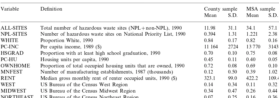
Table 1 contains definitions of all the explana-tory variables (the vectorx from Eq. (1)), as well as descriptive statistics across the two samples (county and MSA). The issue variables are per capita income (PC-INC) and its squared term (PC-INC2). Specifically, the estimated coefficients
on PC-INC and PC-INC2 determine the shape
and position of the EKC. If the quadratic term is negative and the linear term is positive, an
Table 1
Variable definitions and descriptive statistics for count models of EKC relationshipa
Variable Definition County sample MSA sample
Mean S.D. Mean S.D. 11.98 31.1 34.1
ALL-SITES Total number of hazardous waste sites (NPL+non-NPL), 1990 57.1 2.38 0.394 1.31 1.221 NPL-SITES Number of hazardous waste sites on National Priority List, 1990
Proportion White, 1990 0.84 0.17 0.82
WHITE 0.16
13 770
2724 3143
11 164 PC-INC Per capita income, 1989 ($)
Proportion with at least high school graduation, 1990 0.70 0.10 0.75
HSGRAD 0.08
0.45 0.11 0.40 0.05 PC-HU Housing units per capita, 1990
Proportion of total occupied housing units that are owned, 1990 0.72 0.08 0.69
OWNHOME 0.10
0.50
0.12 0.39
Number of manufacturing establishments, 1987 (thousands)
MNFEST 1.02
Median gross monthly rent of renter occupied units, 1990 ($) 323.1 99.0 422.2 109.4 RENT
0.32 0.11
0.34
WEST US Bureau of the Census West Region 0.14
0.34 0.47 0.26 0.44 MIDWEST US Bureau of the Census Midwest Region
0.07 0.25 0.16 0.36 NORTHEAST US Bureau of the Census Northeast Region
aUS per capita income in 1989 was $14 400 (current dollars). The simple average for PC-INC reported here is lower in the county sample. The population-weighted average across counties yields $14 400. Similarly for the MSA sample.
verted-U shaped curve for the data is obtained; i.e. up to a threshold level of per capita income the number of sites increases, but beyond that decreases.
The choice of other explanatory variables is motivated by controlling for factors that may otherwise influence the variation in site data. A set of regional dummy variables (WEST, MID-WEST, NORTHEAST, with SOUTH as the base category) is included to control for the regional disparity in the emergence and location of the types of industries that have heavily influenced the location of hazardous waste sites. Since the de-pendent variable changes with the intensity of production activity across counties, the number of manufacturing establishments (MNFEST) is in-cluded to control for scale effects. A set of vari-ables controlling for socio-economic factors in a region is also included. These variables, which include the proportion of the county population that is White (WHITE), proportion of high school graduates (HSGRAD), per capita housing units (PC-HU), and proportion of owned homes (OWNHOME), distinguish counties by skill and economic status.
Finally, in estimating the generalized NB model an important consideration is the potential endo-geneity of INC term. The distribution of PC-INC across counties may itself be endogenously
determined by the migration decisions of individ-uals, as well as the number of hazardous waste sites. If sites are disamenities, then this effect must be reflected in income differences across regions in a spatial equilibrium (Roback, 1982). Thus, the presence of PC-INC terms in both the NB model of sites and the net outmigration equations (Sec-tion 3) requires a correc(Sec-tion for the endogeneity.3 The method of Kelejian (1971) is used to perform this correction. Fitted values for PC-INC and relevant transformations (i.e. PC-INC2) are gener-ated by regressing these variables on all the right-hand side variables and their squared terms.
2.2. EKC results
The EKC relationship between hazardous waste sites and the set of independent variables was estimated using the generalized NB model. In addition, type 1 NB, type 2 NB, and Poisson models were also estimated separately. The pre-ferred model was selected based on three criteria: the Akaike information criterion (AIC),
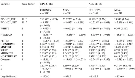
Table 2
Generalized negative binomial model estimates for the EKC relationshipa NPL-SITES
Variable Scale factor ALL-SITES
COUNTY, PC-INC –FIT 10−4 33.239** (5.973) 32.277** (4.714) 18.809** (7.274)
−5.899 (−1.346)
OWNHOME 1 0.067* (0.081)
10.457 (0.867) 35.936** (5.527)
MNFEST 1 0.035 (0.120) −0.240 (−0.600)
0.791 (1.582) WEST 1 2.074** (5.228) 1.205** (4.873) 0.901** (4.536)
0.866** (4.163)
MIDWEST 1 2.093** (5.193) 1.049** (4.072) 0.875 (1.461)
0.979** (11.501) 0.418 (1.100) NORTHEAST 1 1.714** (9.821) 1.011** (4.662)
−0.583 (−0.227)
g 1.533** (7.963) 1.189** (5.220)
−0.340** (−10.069)
Log-likelihood −1929.2 −976.7
0.261 0.560
Maddala’sR2 0.249 0.628
aVariables scaled to be uniform in size. To interpret the coefficients in terms of Table 1 units, scale the estimate by the scale factor. Numbers in parentheses are asymptotict-statistics, computed from the heteroscedastic-consistent covariance matrix. Ifg\0
then there is heterogeneity in variances. The fitted values of PC-INC –FIT and PC-INC2
– FIT are generated by regressing these variables on all the right-hand side independent variables and their squared terms.
* Denotes significance at the 10% level. ** Denotes significance at the 5% level.
hood ratio (LR) tests, and t-tests. The computed LR statistics for NPL sites data (NPL-SITES) favor the generalized NB model over the Poisson
model (LR=686 and 478, respectively, from the
two samples), the type 1 NB model (LR=53 and
27.6), and the type 2 NB model (LR=18, and
13.6). All LR statistics exceed the critical 1% x2 cut-off at 6.64 (1 df). The t-tests also reject the
Poisson hypothesis that g=0, the type 1 NB
hypothesis k=1, and the type 2 NB hypothesis
k=0. A comparison based on the smallest AIC
value, which penalizes excessive parameterization, also favors the generalized NB model. Model comparison diagnostics from the ALL-SITES data also arrive at the same conclusions. Thus, the generalized NB is selected as the preferred model, and used for making inferences.
Evidence of the EKC is presented in Table 2, using the generalized NB model. The first two columns report estimates using NPL site data for the County and MSA samples, respectively. The model fits the cross-sectional NPL data, which is characterized by numerous zero values (58% of the MSA sample and 82% of the County sample have no NPL sites) fairly well. The Maddala’s R2 values are 0.25 for the County sample and 0.26 for the MSA sample, respectively.4
The signs and statistically significant estimates on per capita income and its squared term
(PC-INC and PC-(PC-INC2) bear out the inverted-U
rela-4Maddala’sR2=1−(L
Fig. 1. Fitted EKCs with NPL sites data.
tionship. The EKC from the County sample has a turning point at a per capita income level of $19 375, which is 2.56 S.D. above the sample mean. In our sample of 3141 counties, 1.62% or 36 counties have average per capita incomes that exceed $19 375.5 A review of these counties shows
them to be heavily urbanized high income coun-ties. The EKC from the MSA sample has a turn-ing point at a similar per capita income level of $19 145, which is 1.66 S.D. above the MSA sam-ple mean. In our samsam-ple of 748 MSAs, 6.02% or 42 MSAs have per capita incomes exceeding $19 145. In summary, given the high income turn-ing point, only small percentages of US counties
and MSAs are on the downward slope of the estimated EKC. After controlling for the effects of the other explanatory variables, Fig. 1 presents the fitted EKCs using the NPL sites data for both the County sample and the MSA sample.
Estimated coefficients on other significant ex-planatory variables also have expected signs. Of note, the variable WHITE (proportion of the population that is White) is estimated with a statistically significant negative coefficient in the County sample. This is consistent with the evidence found in Berrens et al. (1997) for hazardous waste generation, and Wang et al. (1998) for the assessed risk of NPL sites.
The last two columns of Table 2 report estimates from the total counts of all hazardous waste sites (ALL-SITES). Since the total data have far fewer zeros than the NPL data, the models fit the cross-sectional data well. Specifically, the total site count data is denser (it has few zeroes; 3% of the MSA sample and 15% of the County sample have no sites). The Maddala’sR2values are 0.56 for the County sample and 0.63 for the MSA sample, respectively. Again the signs and statistical signifi-cance of estimates on per capita income and its
squared term (PC-INC and PC-INC2
), bear out the inverted-U shape of the EKC relationship. Also, the WHITE variable is again estimated with a significant negative coefficient in the County sam-ple.
In the County sample, the EKC turning point occurs at a per capita income level of $17 670, which is 2.15 sample S.D. above the sample mean. In our sample, 3.02% or 95 counties lie on the downward part of the EKC. In the MSA sample, there is only weak evidence of the EKC from the ALL-SITES data, since both the linear and quadratic PC-INC terms are imprecisely measured. Regardless, estimates indicate an income turning point for the EKC of $20 300, which is 1.93 sample S.D. above the sample mean. In our sample, 4.68% or 35 MSAs lie on the downward part of the EKC. Again, given the high income turning point, only small percentages of US counties and MSAs are on
the downward slope of the estimated EKC.6
In summary, the count modeling evidence from all four samples (County and MSA crossed with NPL-SITES and ALL-SITES) indicates the pres-ence of the EKC relationship for hazardous waste sites, with similar per capita income turning points ranging from $17 670 to $20 300.
3. Exploring a migration explanation for the EKC
What is surprising about the existence of the EKC for US hazardous waste sites is that no formal theory advanced so far in the literature is able to explain it. Theories based on shifting of a negative externality (e.g. moving the production of pollu-tion-intensive goods abroad) do not apply to cur-rent hazardous waste sites, which are effectively active until cleaned. The pace of clean-up has been extremely slow. Despite $13 billion in spending through 1992, only 149 NPL sites had completed construction related to their clean-up remedies and only 40 of those sites have been fully cleaned up
(CBO, 1992).7Arguments based on abatement and
incentives to invest in environmentally-friendly technologies (Selden and Song, 1994, 1995) are also
unsatisfactory for hazardous waste sites.
Informal theories have been advanced that public coalitions can exert political influence concerning hazardous waste sites; this is supported by evidence on expansion decisions for treatment, storage and disposal (TSD) facilities (Hamilton, 1993), which are relatively few in number. In contrast, there is no such evidence of collective political influence on speeding the pace of clean-ups (Hird, 1990).
3.1. Migration hypotheses
This study advances and tests a line of argument in which internal migration plays a central explana-tory role behind the observed EKC for hazardous waste sites. The idea that economic mobility lies behind the EKC for hazardous waste sites is also motivated by the work of Mueser and Graves (1995), who examined internal migration
6Although not presented here, the fitted curves using the data for ALL SITES produce inverted-U shaped EKCs similar to those shown for the NPL data (Fig. 1).
within the US over the three decades between 1950 and 1980. In a cross-sectional study of net migration into 520 county aggregates they found strong evidence that amenities are probably as strong a factor in location decisions as employ-ment opportunities. The Mueser and Graves model describes the dynamics of labor movements as the economy moves towards the steady state spatial equilibrium of the earlier static model of Roback (1982).
Mueser and Graves’s model does not differenti-ate by labor quality or social groupings and their migration equations are estimated for the total amount of net migration (separately for each decade). Given the significant negative effect of the WHITE variable in our estimated EKC re-sults, we estimate disaggregated net outmigration rate equations (since sites are disamenities) for two groups: (i) Whites and (ii) a minority group-ing composed of Blacks and Hispanics. A wide variety of factors can affect relative migration rates of different racial and ethnic groups. One possible factor is differences in education and human capital, and hence ex ante economic mo-bility. Another possible factor is the ability to get a conventional home loan mortgage.
Two specific hypotheses are the focus of the analysis. The first specific hypothesis is:
H1: The net outmigration of workers is an
increasing function of hazardous waste sites be-yond a threshold level of per capita income.
IfH1 is valid empirically, then the build-up of hazardous waste sites is not a disamenity source of outmigration until some threshold level of per capita income is crossed. This hypothesis is suffi-cient to produce the inverted-U relationship be-tween income and the number of hazardous waste sites of the EKC. As a simple hypothetical exam-ple, assuming income increases over the life cycle of workers (Mueser and Graves, 1995) and that skill levels are homogeneous across age groups, the proposition implies that beyond a threshold level of income younger workers would drive the left (upward sloping) part of the EKC and older
workers would drive the right (downward
sloping).
The second specific hypothesis is:
H2: The threshold level of income at which net outmigration is influenced by the count of haz-ardous waste sites is the same as the threshold level of income at which the EKC for hazardous waste sites turns downwards.
If H2 holds empirically, it provides a
consis-tency check on the hypothesis that migration is a contributing factor to the observed EKC. If out-migration is influenced by the number of haz-ardous waste sites, then the out-flux of persons above a certain threshold of income to cleaner areas should not be statistically different from the
observed EKC income turning point. To test H1
and H2, we turn to the estimation of a migration model.
3.2. Migration model
In the econometric estimation of the migration equations, net outmigration data across regions (county or MSA) is used for the half-decade
(1985 – 1990) preceding the 1992 EKC data.8
The basic linear model using cross-sectional data on
location i (either county or MSA) is:
NETOMIGRI=b0+b1(SITESi)
+b2(PC-INCi· SITESi)+Zi%L
+oi (2)
where: NETOMIGR is the net outmigration
rate over 1985 – 1990 [(outmigration−
immigra-tion)/population]×100; SITES is the sites
vari-able, which is evaluated separately for
ALL-SITES and NPL-SITES; and similarly in the interaction term, PC-INCi·SITESi, with per capita
income;Zis a vector of socio-economic variables;
b0; b1; b2 and Lare coefficients to be estimated; and o is an error term. We differentiate our find-ings for two groups by separately estimating
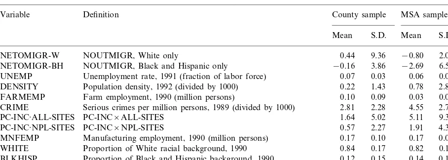
Table 3
Variable definitions and descriptive statistics for migration modelsa
Variable Definition County sample MSA sample
Mean S.D. Mean S.D.
NETOMIGR-W NOUTMIGR, White only 0.44 9.36 −0.80 2.02
−0.16 3.86 −2.69 6.50 NETOMIGR-BH NOUTMIGR, Black and Hispanic only
0.07 0.03
Unemployment rate, 1991 (fraction of labor force) 0.06
UNEMP 0.02
0.22 1.43
DENSITY Population density, 1992 (divided by 1000) 0.78 2.85
0.10 0.09
Farm employment, 1990 (million persons) 0.03
FARMEMP 0.03
Serious crimes per million persons, 1989 (divided by 1000)
CRIME 2.81 2.28 4.55 2.77
1.64 5.02
PC-INC×ALL-SITES 5.11
PC-INC·ALL-SITES 9.36
PC-INC×NPL-SITES
PC-INC·NPL-SITES 0.57 2.27 1.91 4.30
MNFEMP Manufacturing employment, 1990 (million persons) 0.17 0.10 0.17 0.08 0.84 0.17
Proportion of White racial background, 1990 0.82
WHITE 0.16
0.12 0.15
BLKHISP Proportion of Black and Hispanic background, 1990 0.14 0.13 aThe proportion of the US population that was White (non-Hispanic origin) in 1996 was 73.3%. The proportion Black (non-Hispanic origin) was 12.1%. The proportion of Hispanic origin (regardless of current race) was 10.5%. For the county sample, the population-weighted averages of WHITE and BLKHISP are, respectively, 76.2 and 19.38%. Here WHITE includes persons of Hispanic origin, while BLKHISP excludes Hispanics who are White.
els for NETOMIGR-W and NETOMIGR-BH, which denote the net outmigration for Whites (W), and Blacks and Hispanics (BH), respectively. Definitions and descriptive statistics for the vari-ables used in the migration analysis are presented in Table 3.
The test of H1 is based on the estimates for
#NETOMIG-W/#NPL-SITES and #
NETOMIG-W/#ALL-SITES. In reference to the generic Eq.
(2), we have, #NETOMIG-W/#SITES=b1+
b2· PC-INC, which is a function of per capita
income. This response turns positive when PC-INC\(−b1/b2). Thus, we can test H1 by
esti-mating the threshold of per capita income where the response in net outmigration to hazardous
waste sites (i.e. #NETOMIG-W/#NPL-SITES)
turns positive (if at all). The second hypothesisH2
is based on a test of the difference between the level of per capita income at which the EKC turns downwards, with the level of per capita income at
which the response #NETOMIG/#SITES turns
positive.
Explanatory variables (Z) in the outmigration equations are motivated by the four broad factors underlying the Mueser and Graves (1995) specifi-cations. These four factors are: (i) amenities; (ii) employment-related factors; (iii) demographic
fac-tors, and (iv) other regional factors. Amenities are measured by hazardous waste site counts (ALL-SITES or NPL-(ALL-SITES) and rents (RENT). The reason for including RENT as a measure of amenities is that we do not have data on the full variety of amenities such as climate, proximity to recreational locations, air quality, and other qual-ity of life variables. A pragmatic solution in this exploratory context is provided by Graves (1983), who found that rents serve as an excellent proxy for amenities. Hence RENT acts as the ‘com-posite amenity’ following Graves (1983).
Employment-related factors are measured by
manufacturing employment (MFGEMP) and
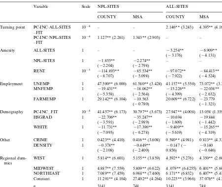
Table 4
White net outmigration rate model (NETOMIGR-W)a
Scale NPL-SITES ALL-SITES
Variable
COUNTY MSA COUNTY MSA
10−4 –
PC-INC·ALL-SITES –
Turning point 2.146** (3.243) 4.395** (4.168)
– FIT
PC-INC·NPL-SITES 10−4 1.127** (2.261) 1.343** (2.903) – – – FIT
1 – –
Amenity ALL-SITES −3.254** −6.909**
(−4.131) (−3.176)
NPL-SITES 1 −1.855** −2.274** – –
(−2.798) (−2.204)
10−3 −114.893** −85.534** −97.072** −84.413** RENT
(−8.707) (−5.098) (−7.922) (−4.524) 1 47.590** (6.000)
Employment UNEMP 61.580** (3.428) 41.157** (5.550) 73.072** (3.306) 1 −19.431**
MNFEMP −18.062** −15.226** −22.038**
(−2.632) (−4.399)
(−2.564) (−5.358)
1 29.142** (6.104) −10.563 20.609** (6.722) −23.779 FARMEMP
(−0.780) (−1.321)
10−4 41.457** (6.173)
Demography PC-INC –FIT 30.797** (3.673) 27.947** (4.008) 13.058 (1.359)
HSGRAD 1 −22.706** −35.247** −10.694 −19.844
(−1.442) (−1.609)
(−2.989) (−3.591)
1 −11.731** −17.396** −9.409** −15.265** WHITE
(−6.278)
(−7.093) (−5.619) (−4.319) Other CRIME 1 0.423** (4.410) 0.416** (3.608) 0.580** (4.981) 0.813** (4.337)
1 −0.378**
DENSITY −0.449** −0.147 (− −0.140
(−0.646) 0.856)
(−2.400) (−2.108)
WEST 1 5.814** (6.601) 5.155** (3.859) 4.592** (5.276)
Regional dum- 4.350** (2.609)
mies
1 4.887** (7.559) 5.809** (6.622)
MIDWEST 4..079** (6.4255) 6.401** (5.601)
1 7.089** (7.459)
NORTHEAST 6.984** (7.460) 6.171** (6.832) 6.407** (5.416) 1 11.291** (4.104) 27.402** (4.264)
Constant 10.225** (3.966) 37.076** (4.321)
3141 748 3141
n 748
0.246 0.288
R2 0.252 0.314
aVariables scaled to be uniform in size. To interpret coefficients in Table 3 units, scale the estimate by the scale factor. Fitted values of PC-INC·ALL-SITES –FIT, PC-INC·NPL-SITES–FIT, and PC-INC–FIT are generated by regressing these variables on all the right-hand side independent variables and their squared terms.
** Denotes significance at the 0.05 level.
measures the upward economic mobility of an area, so that migrants are attracted to areas with high values of HSGRAD. These race/ethnicity variables investigate the attractiveness of living in an area with a similar demographic make-up. Other regional factors include population density (DENSITY) and the crime rate (CRIME), both of which are expected to lead to outmigration. Similar to the EKC estimation, dummy variables
for census regions (West, Midwest, Northeast, with South as the baseline) are included.
3.3. Model results
Table 4 presents OLS estimates from the White net outmigration equation, after again correcting for the endogeneity in PC-INC term by the
0.25 for the County sample and 0.29 for the MSA
sample indicate a fair fit.9 From the estimates
presented in the first two columns of Table 4,
the derivative of interest is #NETOMIG-W/
#NPL-SITES. For the County sample, this
response equals −1.855+1.127×PC-INC
(×10−4). Therefore, #NETOMIG-W/#
NPL-SITES\0 only if PC-INC\1.855/(1.127×
10−4)=$16 460. The inference is that, in the
County sample, net outmigration by Whites in-creases in response to the presence of NPL sites after a threshold level of per capita income of $16 460. At lower levels of income we infer that, after controlling for other socio-economic, re-gional, and amenity factors, NPL sites are not important in location decisions. In the MSA
sam-ple, #NETOMIG-W/#NPL-SITES\0 after per
capita income reaches $16 932. Hence, for the NPL sites, hypothesis H1, that sites emerge as a factor in migration decisions after a certain level of income, is confirmed. This is a necessary condi-tion if migracondi-tion is a contributing factor for the observed EKC.
For total sites,H1is also confirmed. Estimates from the last two columns of Table 4 show that for ALL-SITES the responses are similar. Sites begin to matter beyond a per capita income of $15 163 in the County sample, and $15 720 in the MSA sample.
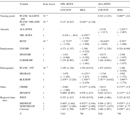
Table 5 presents estimates from the net outmi-gration rates of Blacks and Hispanics taken to-gether. The model fits poorly for the County sample, and the estimates on the coefficients of interest are measured quite imprecisely. This is to be expected because much of the migration in this group is inter-urban migration (Nord, 1998). Hence we focus on the estimates from the MSA sample where the equation has a better fit. In the MSA sample, the coefficients of interest are esti-mated precisely, and afford the inference needed for tests ofH1. Hazardous waste sites are seen to be a factor in the Black and Hispanic net
outmi-gration rate with#NETOMIG- BH/#NPL-SITES
turning positive for PC-INC\$17 537, and
#NETOMIG-BH/#ALL-SITES turning positive
for PC-INC\$15 656. Hence net outmigration is
at levels of income not significantly different from that for Whites.10
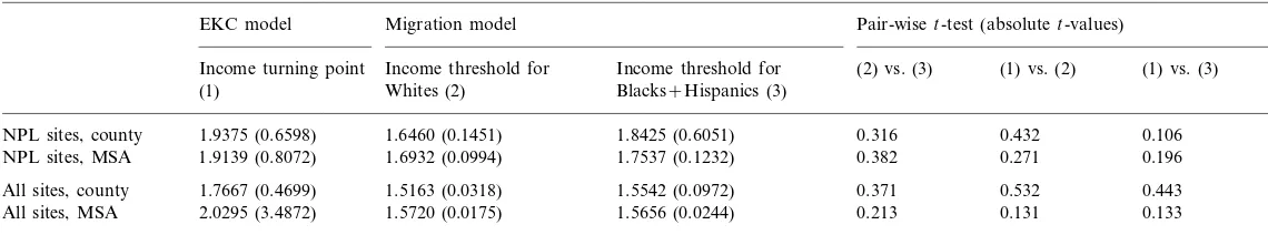
Table 6 collects previous results about income turning points for the EKC, and the threshold
level of income at which #NETOMIG/#SITES
turns positive for all groups, together with their standard errors. This information is used in
test-ing H2 that the income turning points are equal
to the level of income at which the build-up of sites begins to affect outmigration. The last three columns of Table 6 report pairwise t-tests. Con-sider the column labeled ‘(1) vs. (2)’, which tests the equality of the EKC income turning point with the income threshold for White net
outmi-gration. The results support H2: the evidence
indicates no statistical difference. Notably, the income turning points and the income threshold for White net outmigration are both precisely estimated, and failure to find a difference is not due to high standard errors, but rather that the estimates are statistically similar. Other t-tests
from Table 6 also support H2, using the income
thresholds from White net outmigration data or from Black and Hispanic net outmigration data (although the difference of means test for ALL-SITES data for the MSA sample may be influ-enced by the imprecise measurement of the income turning point).
4. Discussion and conclusions
The results of this study provide empirical evi-dence to support the Rothman (1998) hypothesis that a potential contributing factor for observed EKCs may be wealthy households or individuals
distancing themselves from pollution. Using
cross-sectional data and a rigorous count data modeling approach, the EKC is found for
haz-10The result that migration of Blacks and Hispanics re-sponds to environmental quality is consistent with Nord (1998) on the determinants of US county-to-county migration rate over 1985 – 1990 for the working-age poor (which includes a disproportionately large percentage of Black, Hispanics and Native Americans). Nord (1998) emphasizes the disaggregate structure of manufacturing across counties.
Table 5
Black+Hispanic net outmigration rate model (NETOMIGR-BH)a
Variable Scale factor NPL-SITES ALL-SITES
COUNTY MSA COUNTY MSA
PC-INC·ALLSITE 10−4 –
Turning point – 0.332 (1.215) 0.808** (2.841)
– FIT
PC-INC·NPL-SITE 10−4 0.127 (0.627) 0.268** (2.130) – – – FIT
1 –
Amenity ALL-SITES – −0.516 −1.265**
(−2.807) (−1.217)
1 −0.234 (−.685) −0.470**
NPL-SITES − −
(−2.130) 10−3 −11.735**
RENT −7.520* −10.614** −8.795*
(−1.880) (−2.028)
(−1.694) (−2.110)
1 4.371 (1.337) −2.500 UNEMP
Employment 3.977 (1.258) 0.524 (0.094)
(−0.525)
1 −1.011 −1.087
MNFEMP −0.673 −2.308
(−0.441)
(−0.648) (−0.545) (−1.037) FARMEMP 1 1.276 (0.907) −6.190* 1.166 (0.861) −8.694* (−1.857) (−1.661)
10−4 3.199 (1.120) 1.385 (0.613) 1.875 (0.633)
Demography PC-INC –FIT −1.206
(−0.478)
1 −3.079 −8.123**
HSGRAD −1.784 −5.902
(−0.604)
(−1.103) (−2.417) (−1.572) 1 2.874** (5.228) −2.958**
BLKHISP 2.747** (4.882) −3.069**
(−3.775) (−4.479)
1
Other CRIME −0.042 0.113** (3.474) −0.013 0.175** (3.502)
(−0.267) (−1.060)
1 0.0005 (0.007) 0.070 (1.437)
DENSITY 0.022 (0.311) 0.115** (2.108)
WEST 1 0.525 (1.417)
Regional dum- 0.359 (0.979) 0.409 (1.086) 0.223 (0.512)
mies
1 0.443* (1.683) 0.857** (3.636)
MIDWEST 0.369 (1.387) 0.978** (3.335)
NORTHEAST 1 0.846** (2.240) 0.668** (2.680) 0.763** (2.057) 0.536* (1.779) 1 1.421 (1.388) 6.687** (3.993)
Constant 1.646 (1.607) 9.030** (4.235)
3141 748 3141
N 748
0.043 0.174
R2 0.044 0.184
aSee Table 4 notes.
* Denotes significance at the 0.10 level. ** Denotes significance at the 0.05 level.
ardous waste sites in both US counties and MSAs. Further the EKC is found whether using only NPL ‘Superfund’ sites or all hazardous waste sites. Despite the strong evidence for the inverted-U relationship, given the high income turning points only small percentages of US counties and MSAs are on the downward slope of the esti-mated EKCs. Further, using data on internal
Gawande
et
al
.
/
Ecological
Economics
33
(2000)
151
–
166
163
Table 6
Income turning point estimates and tests of equivalencea
Pair-wiset-test (absolutet-values) Migration model
EKC model
Income threshold for Income threshold for (2) vs. (3) (1) vs. (2) (1) vs. (3) Income turning point
Blacks+Hispanics (3)
(1) Whites (2)
1.9375 (0.6598) 1.6460 (0.1451) 1.8425 (0.6051) 0.432 0.106
NPL sites, county 0.316
0.196 1.6932 (0.0994) 1.7537 (0.1232) 0.382 0.271
NPL sites, MSA 1.9139 (0.8072)
1.7667 (0.4699) 1.5163 (0.0318) 1.5542 (0.0972) 0.532 0.443
All sites, county 0.371
0.213 0.131 0.133
1.5720 (0.0175)
All sites, MSA 2.0295 (3.4872) 1.5656 (0.0244)
The results of this empirical study have policy implications for the build-up of hazardous waste sites. There is supportive evidence of a mechanism — internal migration — that underscores the need for geographically-targeted environmental policy. Specifically, if migration is an important factor behind an EKC, then there is the potential for creating pollution enclaves. Further, to the extent that different social groups are differen-tially able to migrate away from areas with critical build-ups of hazardous waste sites, then a migra-tion mechanism is likely to be a source of increas-ing environmental inequity.11
While we do not find evidence of differences in predicted income turning points, to the extent that Whites are more upwardly mobile than Blacks and Hispanics (and achieve certain thresholds earlier in their life-cycle or are more likely to achieve those thresholds), then migration patterns may still exacerbate inequities.
As one policy example, the results of this study offer a measure of support for geographically-targeted clean-ups to correct and further avoid the ‘brownfield’ phenomenon of blighted urban areas with a critical build-up of hazardous waste sites. Brownfields are defined as abandoned, idled or under-used industrial and commercial facilities where expansion or redevelopment is complicated by real or perceived contamination (USEPA, 1998).
We offer our results as an important piece of initial evidence, and thus close with several caveats and suggestions for future research. First, any EKC study is subject to the criticism of being a ‘reduced form’ estimate. However, our results may inform the development of structural models relating economic growth and environmental quality. Various sources have argued that envi-ronmental motivations are an important con-tributing factor in many migration decisions
(Greenwood et al., 1997; Amacher et al., 1998). Thus, these results suggest additional research on whether migration is a causal mechanism behind EKCs for other pollutants. Second, the aggregate nature of our data raises the possibility of an ‘ecological fallacy’, incorrectly inferring micro-level behavior from area aggregate statistics. While we are limited by the nature of our data (which, however, are more disaggregate than the typical EKC study), a suggestion for future re-search is to confirm these findings for hazardous waste sites using aggregate migration data with micro evidence from similar models about individ-ual migration decisions, especially using panel data on migrants.
Appendix A. EKC and migration data
For all variables data was collected at the county level, except for the hazardous waste sites, which were aggregated up from individual site data. There are 3141 counties in the United States, and 748 Metropolitan Statistical Areas consisting of cities with 50 000 or more inhabi-tants. Separate data sets were merged by state-county ‘fips’ code to maintain consistency. EPA’s Landview II Mapping of Selected EPA-Regulated Sites TIGER/LINE 1992 (USEPA, 1992) was the source for hazardous waste data. Regional dum-mies were taken from regions classified by the census. Socio-economic variables (income, racial population, schooling, and housing) were taken from the US Bureau of the Census (1992) STF3A Summary Files. Farm, unemployment, and crime data were collected from the 1996 USA Counties CD-ROM by the US Bureau of the Census (1996). Manufacturing data are from the 1994 County and City Data Book (US Bureau of the Census, 1994).
The migration data are based on cross-sectional data obtained from the 1990 census long form questionnaire, distributed to approximately 17% of US households. Respondents were asked where they lived in 1985, and where they currently resided. The number of people who reported a different county of residence in 1990 compared with 1985 determined the number of migrants.
This data are available on two complementary CD-ROMs, the County to County In-Migration Flow File (US Bureau of the Census, 1995a) and the County to County Out-Migration Flow file (US Bureau of the Census, 1995b). The former reports all flows into a county between 1985 and 1990, while the latter reports all flows out of a county between 1985 and 1990. The difference between the latter and the former yields net out-migration between 1985 and 1990 for any given county.
References
Amacher, G., Cruz, W., Grebner, D., Hyde, W., 1998. Envi-ronmental motivations for migration: population pressure, poverty, and deforestation in the Philippines. Land Econ. 74, 92 – 101.
Arrow, K., Bolin, B., Costanza, R., Dasgupta, P., Folke, C., Holling, C., Jansson, B., Levin, S., Maler, K., Perrings, C., Pimentel, D., 1995. Economic growth, carrying capacity, and the environment. Science 268, 520 – 521.
Beckerman, W., 1992. Economic growth and the environment: whose growth? whose environment? World Dev. 20, 481 – 496.
Berrens, R., Bohara, A., Gawande, K., Wang, P., 1997. Test-ing the inverted-u hypothesis for US hazardous waste sites: an application of the generalized gamma model. Econ. Lett. 55, 435 – 440.
Cavlovic, T., Baker, K., Berrens, R., Gawande, K., 2000. A meta-analysis of environmental Kuznets curve studies. Agric. Resour. Econ. Rev. (in press).
Congressional Budget Office (CBO), 1992. The total costs of cleaning up non-federal Superfund sites. US Government Printing Office, Washington, DC.
Farber, S., 1998. Undesirable facilities and property values: a summary of empirical studies. Ecol. Econ. 24, 1 – 24. Graves, P., 1983. Migration with a composite amenity: the role
of rents. J. Reg. Sci. 23, 541 – 546.
Greenwood, M., Hunt, G., 1989. Jobs versus amenities in the analysis of metropolitan migration. J. Urban Econ. 25, 1 – 16.
Greenwood, M., McClelland, G., Schulze, W., 1997. The effects of perceptions of hazardous waste on migration: a laboratory experimental approach. Rev. Reg. Stud. 27, 143 – 161.
Grossman, G., Krueger, A., 1993. Environmental impacts of a North American free trade agreement. In: Garber, P. (Ed.), The US-Mexico Free Trade Agreement. MIT Press, Cam-bridge, MA.
Grossman, G., Krueger, A., 1995. Economic growth and the environment. Q. J. Econ. 112, 353 – 378.
Grossman, G., Krueger, A., 1996. The inverted-u: what does it mean? Environ. Dev. Econ. 1, 119 – 122.
Gupta, S., Van Houtven, G., Cropper, M., 1996. Paying for permanence: an economic analysis of EPA’s clean-up deci-sions at Superfund sites. Rand J. Econ. 27, 563 – 582. Gurmu, S., Trivedi, P., 1996. Excess zeros in count models. J.
Bus. Econ. Stat. 14, 469 – 477.
Hamilton, J., 1993. Politics and social costs: estimating the impacts of collective action on hazardous waste facilities. Rand J. Econ. 24, 101 – 125.
Hird, J., 1990. Superfund clean-up expenditures: distributive politics or the public interest. J. Policy Anal. Manag. 9, 455 – 483.
Holtz-Eakin, D., Selden, T., 1995. Stoking the fires? CO2 emissions and economic growth. J. Public Econ. 57, 85 – 101.
Kaufmann, R., Davidsdottir, B., Garnham, S., Pauly, P., 1998. The determinants of atmospheric SO2 concentra-tions: reconsidering the environmental Kuznets curve. Ecol. Econ. 25, 195 – 208.
Kelejian, H., 1971. Two stage least squares and econometric systems linear in parameters but non-linear in the endoge-nous variables. J. Am. Stat. Assoc. 66, 373 – 374. McConnell, K., 1997. Income and the demand for
environ-mental quality. Environ. Dev. Econ. 2, 383 – 399. Mueser, P., Graves, P., 1995. Examining the role of economic
opportunity and amenities in explaining population redis-tribution. J. Urban Econ. 37, 176 – 200.
Nord, M., 1998. Poor people on the move: county-to-county migration and the spatial concentration of poverty. J. Reg. Sci. 38, 329 – 351.
Roback, J., 1982. Wages, rents, and quality of life. J. Polit. Econ. 90, 1257 – 1277.
Rothman, D., 1998. Environmental Kuznets curves – real progress or passing the buck?: a case for consumption-based approaches. Ecol. Econ. 25, 177 – 194.
Selden, T., Song, D., 1994. Environmental quality and devel-opment: is there a Kuznets curve for air pollution? J. Environ. Econ. Manag. 27, 147 – 162.
Selden, T., Song, D., 1995. Neoclassical growth, the j curve for abatement and the inverted-u curve for pollution. J. Envi-ron. Econ. Manag. 29, 162 – 168.
Shafik, N., 1994. Economic development and environmental quality: an econometric analysis. Oxford Econ. Papers 46, 757 – 773.
Shafik, N., Bandyopadyhay, S., 1992. Economic growth and environmental quality: time series and cross-country evi-dence. World Bank, Washington, DC background paper for the World Development Report.
Suri, V., Chapman, D., 1998. Economic growth, trade and energy: implications for the environmental Kuznets curve. Ecol. Econ. 25, 195 – 208.
Torras, M., Boyce, J., 1998. Income, inequality, and pollution: a reassessment of the environmental Kuznets curve. Ecol. Econ. 25, 147 – 160.
US Bureau of the Census, 1994. County and City Data Book, 1994 on CD-ROM. US Bureau of the Census, Washing-ton, DC.
US Bureau of the Census, 1995a. Census of Population, 1990: County to County In-Migration Flow File on CD-ROM. US Bureau of the Census, Washington, DC.
US Bureau of the Census, 1995b. Census of Population, 1990: County to County Out-Migration Flow File on CD-ROM. US Bureau of the Census, Washington, DC.
US Bureau of the Census, 1996. USA Counties 1996 on CD-ROM. US Bureau of the Census, Washington, DC.
US Environmental Protection Agency (USEPA), 1992. Land-View II Mapping of Selected EPA-Regulated Sites, Tiger/
Line. USEPA, Washington, DC.
US Environmental Protection Agency (USEPA), 1998. Brownfields’ Fact Sheet. Office of Solid Waste and Emer-gency Response, USEPA, Washington, DC Publication 500-F-98-001.
Wang, P., Berrens, R., Bohara, A., Gawande, K., 1998. An environmental Kuznets curve for risk-ranked US haz-ardous waste sites. Appl. Econ. Lett. 5, 761 – 764. Zimmerman, R., 1993. Social equity and environmental risk.
Risk Anal. 13, 649 – 665.