A Spatio-temporal Model of Farmland
Values
David Maddison
1(Original submitted November 2007, revision received August 2008, accepted September 2008.)
Abstract
Despite the fact that data on farm sales are invariably collected over both time and space, previous papers have allowed for the presence of either temporal or spa-tial relationships in the data, but not both. Some papers have also inadvertently assumed that although farmland values are influenced by prices realised by nearby sales, these sales need not necessarily be comparable in terms of their attributes. Using data on sales of farmland obtained through public auctions in England and Wales, this paper examines the consequences of explicitly allowing for the pres-ence of a spatio-temporal lag in the estimation of hedonic models of farmland value. The results indicate that spatio-temporally lagged values of the dependent and independent variables contribute significant additional explanatory power. Accounting for spatio-temporal relationships appears moreover to somewhat alter the perceived size and statistical significance of key farmland attributes.
Keywords: Farmland prices; hedonic analysis; spatial econometrics; spatio-tem-poral.
JEL classifications:C31,Q11,Q51.
1. Introduction
The hedonic (or Ricardian) technique has been widely used to value farmland ame-nities. It involves regressing variables related to the structural and environmental characteristics of farmland on the rental value or sale price per unit area. Any dif-ferences in market values arising from difdif-ferences in the abundance of key farmland characteristics are attributed to the productive value of those characteristics when the land is put to its most profitable use, given current input and output prices. The theory underlying the hedonic model applied to agricultural land is well understood (see, e.g. Palmquist, 1989 or Freeman, 1993 for an exposition).
Using this method, researchers have investigated the value of soil quality (Mira-nowski and Hammes, 1984); investments in drainage (Palmquist and Danielson,
1
David Maddison is based in the Department of Economics, University of Birmingham, Edgbaston, Birmingham B15 2TT, UK. Tel.: +44 (0)121 414 6653, Fax: +44 (0)121 414 7377, E-mail: [email protected]
1989); top-soil depth (Brown and Barrow, 1985); measures to stem soil erosion (Ervin and Mill, 1985); eligibility for government schemes (Nickerson and Lynch, 2001); the availability of water (Mendelsohn and Dinar, 2003); and the value of cli-mate variables (Mendelsohnet al., 1994; Reinsborough, 2003).
Many of the farmland attributes valued by previous researchers using the hedonic technique are spatially autocorrelated and vary significantly only over large geo-graphical distances. Farmland attributes not observed by the researcher but never-theless important to farmland productivity might also vary comparatively little over short distances. Examples of important non-observed characteristics include the nebulous but potentially important ‘distance to market’ and ‘land development potential’. Currently, such factors are often controlled for by distance to the nearest city or by the population density of the county in which the farmland is located, although neither of these controls is adequate given the arbitrariness of deciding what constitutes a city, much less a market.2
Individual farmers or institutional investors contemplating land purchases might also place considerable weight on the price information generated by earlier sales and in particular by the sale of nearby plots. Although such behaviour is at odds with the idea underlying the hedonic technique, namely that farmers have the per-fect information and care only about the characteristics of the plot, such behaviour might be sensible when the collection of information is a costly activity. According to Can (1992), such behaviour takes the form of seeking ‘comparable’ sales in ear-lier time periods.3
Noting the potential bias in parameter estimates that arises when these and related issues are ignored, Bell and Dalton (2007) point out that controlling for spa-tial effects in studies necessitates a range of analytical modifications to hedonic analyses. A failure to account for spatial phenomenon might lead to a violation of the assumptions required to establish the optimal properties of ordinary least squares (OLS), properties upon which hedonic analyses frequently depend. (For evi-dence on the propensity of spatially autocorrelated residuals to exaggerate the sig-nificance levels for any spatially autocorrelated explanatory variables, see Kramer and Donninger, 1987.)
Despite the relatively large number of papers valuing farmland characteristics, few studies of farmland value have so far adopted an explicitly spatial perspective.4 Such techniques are nevertheless becoming more widespread in the analysis of resi-dential land markets. Examples include those of Pace and Gilley (1997), Basu and Thibodeau (1998), Tse (2002) and Kim et al. (2003). (For a general discussion of the use of spatial statistics in real estate, see Pace et al., 1998a.) Benirschka and Binkley (1994) explain the variation in county-wide agricultural land prices while accounting for the fact that the residual values for observations drawn from neigh-bouring counties are likely to be autocorrelated. Vandeveer et al. (1998) use Geo-graphical Information Systems to illustrate the presence of spatial autocorrelation
2
See Dubin (1992) for a further discussion of the concept of ‘sliding neighbourhoods’. See also Clonts (1970).
3
By ‘comparable’ I mean comparable in terms of plot characteristics. 4
in agricultural land prices. This visual evidence is reinforced by formal tests of spa-tial autocorrelation. Patton and McErlean (2003) found evidence of spaspa-tial relation-ships in their analysis of agricultural land prices in Northern Ireland. They allege that agricultural land prices are characterised by a simultaneous spatial lag, which they subsequently attribute to individuals relying on the price of adjacent plots of land as a guide.5,6 In their study of the disamenities caused by large-scale animal operations and mushroom production, Ready and Abdalla (2005) account for spa-tial autocorrelation in their hedonic house price study.
The contribution of this paper is to extend the hedonic model of farmland values to one in which spatio-temporal relationships are present. More specifically, the model presented here assumes that the price of farmland is affected by a spatially weighted average of sale prices achieved during past time periods, arguing that Pat-ton and McErlean’s implicit assumption of a simultaneous spatial lag is an implau-sible representation of the market price formation process. Individuals contemplating the purchase of farmland can use only the past as a guide, not the future. The model presented in this paper further allows for the possibility that the characteristics of spatio-temporally lagged sales might be important in determining the extent to which they serve as comparables. In making these changes, the paper pays much closer attention than did previous researchers to the manner in which land markets appear to function.
Anticipating the main results of the paper, adding spatio-temporally lagged values of farmland values as well as terms describing the characteristics of those sales generates a highly significant improvement in explanatory power. At the same time, that statistical significance of key farmland attributes appears to change. Finally, calculating the value of farmland amenities is far easier than in a model character-ised by a simultaneous spatial lag. Such findings are of great concern to those seek-ing to use hedonic analysis to measure the value of farmland attributes accurately.
It is important to note that although it has a temporal component, the purpose of this paper is not to explain the evolution of farmland prices over time. That is the pur-pose of models methodologically quite different in outlook to the one presented here in which dummy variables are used to absorb all macroeconomic influences. The focus is purely on hedonic models and how previously unexplained cross-sectional variation in farmland values can be reduced and the risk of potential bias lessened by including spatio-temporally lagged values of the dependent and independent variables.7
The remainder of the paper is organised as follows. Section 2 offers a suitably brief review of the relevant aspects of spatial econometrics while at the same time directing the reader to more detailed references in the literature. Section 3 describes the dataset upon which the model is estimated. Section 4 presents a series of
5
See also Maddison (2004) and Patton and McErlean (2004).
6There are also a number of spatial analyses or discussions relating to the applicability of spatial techniques to agriculture but not involving farmland values. Examples include Bockst-ael (1996), Weiss (1996), Nelson and Hellerstein (1997), Irwin and BockstBockst-ael (2002) and Roe et al.(2002). Hollowayet al. (2007) provide an excellent survey of the literature. Florax and Van der Vlist (2003) give an overview of the more general application of spatial econometric techniques.
7
econometric models and section 5 presents a new spatio-temporal model of farm-land values, which is then formally compared with a model characterised by a simultaneous spatial lag. The final section concludes.
2. Spatial Econometrics
Given the several recent reviews of the spatial econometrics literature, the review provided here will be brief.8
Spatial data may present itself in a variety of forms. Data can be observed at irregularly spaced points on a two-dimensional surface. Alternatively, spatial data can refer to geographical areas, some of which may be contiguous to other units.
Spatial relationships in regression analyses involving such data can also be mod-elled in a variety of ways. Spatial lags hypothesise that the value of the dependent var-iable observed at a particular location is partially determined by a spatially weighted average of the value of the dependent variable as measured at other locations. Such a model cannot be estimated by OLS because of the problem of simultaneity bias and must instead be dealt with using either instrumental variable estimators or maximum likelihood techniques. The spatial lag model in matrix form is given by:
Y¼aþXbþqWYþe ð1Þ
whereYis a (n ·1) vector of dependent variables,Xa (n ·k) matrix of explanatory variables, Wis the (n·n) spatial weight matrix,a andq are scalar parameters and b is a (k·1) vector of parameters.
A number of different assumptions can be made concerning the spatial weights matrix required to compute the spatially weighted values at each location. One pos-sibility is that the weights matrix should merely identify the nearest neighbour or n nearest neighbours. An alternative is that the weights matrix should identify those observations located within an arbitrarily fixed distance. A third alternative is that the weights matrix contains the inverse geographical distances between observations or some function thereof. In instances in which data refer to geographical areas as opposed to points on a plane it is customary to construct a contiguity matrix indi-cating which geographical areas are adjacent to one another. Weights matrices are commonly row-standardised such that their rows sum to unity and have zeros along the leading diagonal.
Calculating the impact of marginal changes in the value of the independent vari-ables in the spatial lag model is not as straightforward as it might first appear. The reason is that changes in the independent variables have both direct and indirect feedback effects on the value of the dependent variable. This fact can best be appre-ciated by solving the spatial lag model forYto obtain:
Y¼ ðIqWÞ1Xbþ ðIqWÞ1e ð2Þ This is an important point to which I shall return.
8
An alternative form of spatial relationship occurs when the dependent variable can also be predicted as a function of spatially lagged values of the independent variables. Unlike spatial lags, this model can be estimated using OLS. The spatial regression model is given by:
Y¼aþXbþWXcþe ð3Þ
wherecis a (k·1) vector of coefficients.
The final way of incorporating spatial relationships is through spatial dependence in the error term. This can be in the form of spatially autoregressive errors or a spa-tial moving average. The spaspa-tial error model is given by:
Y¼aþXbþe ð4Þ
where
e¼kWeþu ð5Þ
andk is a scalar parameter. Such models can be estimated through feasible general-ised least squares or maximum likelihood techniques.
A distinction can be drawn between spatio-temporal and simultaneous spatial relationships. In spatio-temporal models, the observations are ordered in time such that spatially lagged values of current dependent and independent variables are allowed to influence only the future realisations of random variables. For the pur-poses of this paper, the distinction between these two types of model is very impor-tant. Calculating the marginal impact of changes in the independent variables is also much easier in the context of a spatio-temporal model.9 (For an introduction to spatio-temporal models, see Paceet al., 1998b.)
Spatial relationships in the data typically violate the assumptions underlying OLS, leading either to inefficiency and invalid hypothesis testing procedures or even to bias and inconsistency in the parameter estimates. The specification of spatial models can proceed either on the basis of diagnostic tests or on the basis of theoret-ical reasoning. Another important consideration is that simultaneously modelling several forms of spatial relationships such as the spatial lags and a spatially auto-regressive error term is not possible at present. A final consideration is that whereas several tests are available that indicate whether spatial relationships are present in data, some of these tests have difficulty in discriminating between different forms of spatial relationship.
3. Data
The dataset used to test for the presence of spatio-temporal relationships in agricul-tural land prices and to illustrate the consequences of failing to account for such relationships comprises observations on farmland transactions that occurred in Eng-land and Wales from the beginning of January 1994 to the end of June 1996. These are taken from the twice-yearly publicationFarmland Market. In total, 601 observa-tions are available for analysis although in order to generate a spatio-temporal lag (see below) the first six months worth of data (94 observations) are kept in reserve.
9
A shortcoming of the dataset is that only those sales taking place through public auction are included in the analysis. But as a record of farms sold through public auction, the dataset is almost complete.10 Moreover, the sale of land through public auction rather than private transaction generates precisely the kind of infor-mation externality that was earlier argued to give rise to spatio-temporal relations in the data.
The dataset includes the current sale price of the farmland (PRICE) measured in pounds sterling and also the size of the farm (ACRES) in acres. Many sales have large farmhouses attached to them. Usually information is available only on the number of bedrooms, and the presence of other agricultural buildings is not recorded systematically. The number of bedrooms is divided by the number of acres (BEDS⁄ACRES) to provide an indicator of the level of structural attributes per unit of land. Animals and agricultural equipment are typically sold separately from the land and its buildings. The observations are geographically referenced using the Ord-nance Survey gazetteer (a database of all place names in Britain and their spatial coordinates). Observations, whose location could not be determined to a satisfactory degree of precision, were discarded. Repeat sales of land were also discarded.
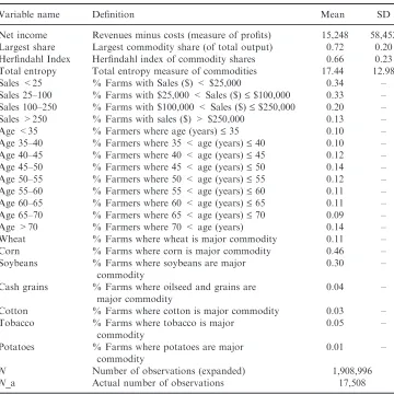
Consistent with previous studies, a variable is included denoting the distance in kilometres to the nearest city, partly as a measure of distance to market and partly as a measure of development potential. A city is variously defined with at least 250,000 people to obtain the variable DIST250 or with at least 100,000 people to obtain the variable DIST100. Note that there are 17 cities with a population size in excess of 250,000 in Great Britain and 57 cities with a population size in excess of 100,000. A referee remarks that proximity to smaller urban areas might also be important. The problem about including a variable indicating proximity to urban areas with a population of significantly less than 100,000 is that the variation in the resulting variable is sharply diminished. Observe already the difference in the stan-dard deviation between variables DIST250 and DIST100 in Table 1. Alternately put, nowhere in England or Wales is very far from a community of 10,000 or more. Following Shi et al. (1997), I also create a variable URBAN which takes into
Table 1
The dataset
Variable Mean SD Minimum Maximum
PRICE⁄ACRES 2,814 1,441 154 12,571
ACRES 84 148 7 2,794
BEDS 1.14 2.06 0 11
ALC 3.00 0.82 1 5
DIST250 57 38 5 211
DIST100 36 20 2 123
URBAN 5,867 2 5,866 5,900
10
account both geographical distances and the population size of nearby cities. This involves calculating for each ploti and for each cityjof at least 100,000 people the following variable:
URBANi¼X j
POPj=DIST2
ij ð6Þ
where POP is the population of city j·100,000 and DIST is the distance between plotiand city jin kilometres. Including these variables does not of course preclude the possibility that the spatial techniques employed below will prove better at mod-elling the twin influences of distance to market and development potential.
A series of land-quality variables were matched to the data using the geographical coordinates of the farmland sold. The 5-km grid square agricultural land classifica-tion (ALC) system of England and Wales classifies land into one of five different grades (Ministry of Agriculture Food and Fisheries, 1988). The land-grading system is based on the extent to which among other things, climate, physical composition, drainage characteristics and slope impose long-term limitations on lands’ agricul-tural use. Grade 1 agriculagricul-tural lands are the best and grade 5 the worst. The same dataset also records if land was non-agricultural in nature or simply not surveyed in which case it is dropped from the dataset.
The obvious disadvantage of the ALC is that it fuses together a number of char-acteristics, making it impossible to determine the individual contribution any given characteristic makes to farmland productivity. The advantage of using the classifica-tion is that it is the result of many years of fieldwork and is available at a high level of spatial resolution. As using data at a low level of spatial resolution can itself result in spatial autocorrelation and because the focus of this paper is primarily methodological, on balance it was deemed appropriate to use the classification as the sole measure of farmland productivity.
The most natural way of incorporating the land quality data is obviously to include four dummy variables corresponding to the different land classifications, along with the constant term. But in what follows, a single variable taking integer values from 1 to 5 was included in the model. This is because the majority of land is classified as either grade 3 or 4 and because including separate dummies for each land classification did not result in a statistically significant improvement in fit in any of the regression models presented below.
Finally, dummy variables DUM1, DUM2 and DUM3 identify the periods Janu-ary 1995 to June 1995, July 1995 to December 1995 and JanuJanu-ary 1996 to June 1996, respectively. The constant term refers to the period July 1994 to December 1994. The purpose of these dummy variables is to account for changes in the cur-rent price of inputs and outputs as well as future expectations regarding these things. Changes in price expectations are clearly very important in determining the value of land and failing to control for these risks obscuring the value of farmland attributes. The dataset is described in Table 1.
calculations, it is convenient to assume that the individual elements (wij) of the weight matrix evolve according to:
wij ¼1=dfij ð7Þ
where the exponent f is often referred to as the friction parameter and dij are the elements of D.11 The leading diagonal of the weights matrix W is filled with zeros and the matrix is then row-standardised such that the rows of the matrix each sum to unity. An alternative assumption is to compute a standardised binary spatial weight matrix identifying those farms which lie within a pre-specified distance of one another. Unfortunately, the largest minimum distance between sales contained in the dataset (74 km) limits the usefulness of this approach. But by increasing the size of the friction parameter, the weight placed on more distant farms can be made arbitrarily small and does away with the need to specify a distance limit. I have examined different values for fand find that the inverse distance model with f= 1 yields the most pronounced evidence of spatial dependence.
4. Econometric Results
The presence of spatial autocorrelation in the data is confirmed using Geary’s C-statistic (Geary, 1954). The results of these tests are presented in Table 2 and indicate that as might be anticipated, the variables PRICE⁄ACRES and ALC are significantly autocorrelated over space. The level of structural attributes per unit of land BEDS⁄ACRES is spatially autocorrelated at the 5% level of confidence and ACRES is not spatially autocorrelated. The fact that some explanatory variables are highly spatially autocorrelated, whereas others are not, suggests that accounting for spatial effects might have a differential impact on the perceived size and statisti-cal significance of these variables.
Using an alternative approach to examine the range of spatial autocorrelation, a series of binary standardised spatial weight matrices were created identifying neigh-bouring farms that fall within, e.g. 0–75, 75–150, 150–225 km of one other. Com-puting Geary’s C-statistic for each of these binary spatial weight matrices suggests that the price per acre of farms within 150 km of each other exhibits statistically significant positive spatial autocorrelation and that for farms within 75 km of each other this statistical relationship is highly significant. This same test is also con-ducted using cumulated distance, i.e. for farms that fall within 0–75, 0–150,
Table 2
Global spatial autocorrelation statistics
Variable Geary’sC Probability
PRICE⁄ACRES 0.939 0.000
ALC 0.846 0.000
BEDS 0.978 0.010
ACRES 1.042 0.253
Note:Spatial weight matrix = inverse distance row-standardised.
0–225 km of one another. This suggests spatial autocorrelation even up to a range of 225 km. Note that the probability values given in Table 3 refer to a one-tailed test.
To begin with, various special cases of the following model are estimated:
log(PRICE/ACRES)¼aþb1ACRESþb2ALCþb3(BEDS/ACRES) þb4(BEDS/ACRES)2þb5DIST250þb6DIST100 þb7URBANþb8DUM1þb9DUM2
þb10DUM3þqXwilog(PRICE/ACRES)iþe ð8Þ where:
e¼kXwieiþu ð9Þ
and a, b1–10, q and k are the parameters. Note that the dependent variable was taken as the log of PRICE⁄ACRES following attempts to estimate a Box–Cox transformation of the dependent variable. Taking PRICE⁄ACRES as a purely lin-ear variable resulted in an equation which did not pass the RESET test for func-tional form (Ramsey, 1969). For the same reason, it was necessary to add a quadratic term for BEDS⁄ACRES. The number of acres was included as an explan-atory variable in case repackaging of land is a costly activity.12
Setting the parametersq andk equal to zero yields the usual hedonic price equa-tion estimable by OLS. Allowing the parameter q to vary results in a model in which individual sale prices are affected by the prices of neighbouring properties. Allowing the parameter k to vary results in a model where the residuals are auto-correlated over space.13
The regression results are presented in Table 4 in which the conventional hedonic model estimated by OLS withq andk are set equal to zero. Note that thet-statistics
Table 3
Banded measures of spatial correlation
Distance (km) Geary’sC Distance (km) Geary’sC
0–75 )5.493 (Prob = 0.000) 0–75 )5.493 (Prob = 0.000) 75–150 )1.828 (Prob = 0.034) 0–150 )3.940 (Prob = 0.000) 150–225 )0.275 (Prob = 0.392) 0–225 )1.815 (Prob = 0.035) 225–300 1.298 (Prob = 0.097) 0–300 0.020 (Prob = 0.492) 300–375 )0.078 (Prob = 0.469) 0–375 1.276 (Prob = 0.101) 375–450 )0.650 (Prob = 0.258) 0–450 1.095 (Prob = 137) 450–525 )0.657 (Prob = 0.256) 0–525 0.903 (Prob = 0.183) 525–600 )0.534 (Prob = 0.297) 0–600 0.729 (Prob = 0.233)
Notes:Spatial weight matrix = inverse distance row-standardised. Variable = PRICE⁄ACRE.
12
The so-called ‘linearity hypothesis’ (Parsons, 1990) would imply taking the dependent vari-able PRICE in levels and multiplying any environmental attributes like ALC by the number of acres. Here I prefer to take the dependent variable as price per acre in order to reduce het-eroscedasticity so I divide the structural attribute BEDS by the number of acres.
are based upon robust standard errors. The results reveal that as land quality wors-ens the price of land declines. The results also indicate that the greater the number of bedrooms per acre the greater the price albeit at a diminishing rate. Smaller plot sizes command a higher price per acre indicating that the repackaging of land is a costly activity. Turning now to the alternative measures of distance to market cum urban development potential, defining a city in terms of an urban area with a population in excess of 250,000 is by far the most successful strategy in terms of fit. This variable is negatively signed as anticipated, and highly significant. By contrast, DIST100 and URBAN are jointly insignificant and dropped from all further regressions.14
Before conducting any spatial regressions, an important issue to address is whether the regressions are stable across different regions or whether geographically distinct markets exist, within which the implicit prices of farmland characteristics differ (Straszheim, 1974). Freeman (1993) explains the circumstance under which geographically segmented markets arise: when buyers do not, for whatever reason, participate in different markets while at the same time these regions differ in terms of the supplies of and demands for attributes.
When markets are segmented but model intercepts and coefficients are con-strained to be the same, market segmentation can manifest itself in positive tests for spatial autocorrelation. There is however no prior information to indicate the areas that might potentially be considered separate markets, and furthermore the sample size is of modest dimensions. These considerations suggest that the most appropri-ate strappropri-ategy is to use the dummy variable approach to allow the intercept and slopes of the regression equations to differ across each of four quadrants referring to the
Table 4
The regression results for the OLS model
Variable Parameter (t-stat) Parameter (t-stat)
CONSTANT 61.819 (1.81) 8.165 (110.69)
ACRES )0.000793 ()6.31) )0.000794 ()6.34)
ALC )0.132 ()5.98) )0.137 ()6.34)
BEDS⁄ACRES 11.359 (13.84) 11.288 (13.80) (BEDS⁄ACRES)2 )20.609 ()10.24) )20.591 ()10.28) DIST250 )0.00281 ()3.80) )0.00303 ()4.89) DIST100 )0.00142 ()1.28)
URBAN )0.00913 ()1.57)
DUM1 0.2183 (4.64) 0.220 (4.68)
DUM2 0.295 (5.83) 0.297 (5.87)
DUM3 0.355 (6.99) 0.352 (6.97)
F-statistic 87.74 (Prob=0.000) 103.38 (Prob=0.000)
No. obs. 507 507
R2 0.407 0.405
RESET 0.05 (Prob=0.983) 0.11 (Prob=0.951)
Notes:Dependent variable = log(PRICE⁄ACRES). Method = OLS.
t-statistics are heteroscedastic-consistent.
south-east (SE), the north-east (NE), the north-west (NW) and the south-west (SW). The coefficients relating to these geographically defined sub-markets are pre-sented in Table 5. The test for parameter stability is significant at the 1% level of confidence, implying that the hypothesis of a market for farmland, unified by trade in agricultural commodities, must be abandoned.15 Across the four sub-markets, several important differences are observed in the implicit values of farmland charac-teristics. In the SE and the SW, the price per acre is not affected by farm size. In the SE, high-quality farmland does not attract a premium possibly because it is rel-atively more abundant there. Alternrel-atively, the value of agricultural land grade 3, 4 and 5 may be higher in the SE because of the greater developmental opportunities typically denied to prime agricultural land or because of the higher recreational and environmental values in part related to the higher population and greater wealth of the SE. Finally, distance to the nearest big city is an amenity only for farms in the NW and SW of the country.
Table 6 displays test results for spatial error and spatial lag dependence in the OLS model with heterogeneous land markets. The Lagrange multiplier tests are less useful in this respect because each test has some power against the alternative form of spatial dependence. The robust Lagrange multiplier tests overcome this problem (Anselinet al., 1996). Both the robust and the non-robust versions of the test statis-tics point to the existence of a spatial lag.16 There is no evidence that spatial auto-correlation is due to omitted neighbourhood characteristics (the tests for spatial error dependence are statistically insignificant).
Table 5
The regression results for the OLS model with regional land markets
Variable
CONSTANT 7.708 (43.81) 8.0380 (55.88) 8.690 (39.20) 7.911 (55.12) ACRES 0.000117 (0.31) )0.000901 ()5.55) )0.000678 ()2.27) )0.000944 ()1.47) ALC )0.0281 ()0.58) )0.116 ()2.86) )0.259 ()4.03) )0.0902 ()2.41) BEDS⁄ACRES 11.285 (3.56) 11.621 (9.13) 10.960 (2.89) 7.172 (2.00) (BEDS⁄ACRES)2 )6.212 ()0.22) )22.526 ()7.47) )23.920 ()0.55) 24.868 (0.78) DIST250 0.000127 (0.09) 0.000004 (0.00) )0.00343 ()3.12) )0.00321 ()2.93) DUM1 0.0901 (1.14) 0.269 (3.17) 0.247 (2.08) 0.1403 (1.66) DUM2 0.167 (2.21) 0.149 (1.55) 0.278 (2.06) 0.503 (5.41) DUM3 0.147 (1.71) 0.380 (4.16) 0.428 (3.59) 0.424 (4.51)
F-statistic 50.52 (Prob=0.000)
No. obs. 507
R2 0.486
RESET 1.34 (Prob=0.260)
Notes:Dependent variable = log(PRICE⁄ACRES). Method = OLS.
t-statistics are heteroscedastic-consistent.
15
F(27, 471) = 3.92. 16
Table 7 presents the same regression equation but with spatial lag dependence (q allowed to vary butk is set equal to zero). The parameter estimates are not much altered but the spatial autocorrelation parameter q is highly significant.17 The results from this model are very similar to those from the heterogeneous land mar-ket model without a spatial lag except that distance to the nearest big city is no longer significant in the NW whereas previously it was significant at the 1% level of confidence. But it is important to avoid believing that because the parameter coeffi-cients are similar that the implicit value of marginal changes in the value of the dependent variables must also be similar. The preceding section illustrated that
Table 6
Tests of spatial autocorrelation in the OLS model
Spatial error dependence
Moran’sI-statistic 3.631 (Prob=0.000) Lagrange multiplier test 2.191 (Prob=0.139) Robust Lagrange multiplier test 2.910 (Prob=0.088) Spatial lag dependence
Lagrange multiplier test 9.134 (Prob=0.003) Robust Lagrange multiplier test 9.852 (Prob=0.002)
Note:Spatial weight matrix = inverse distance row-standardised.
Table 7
The regression results for the spatial lag model
Variable
CONSTANT 2.013 (1.21) 2.320 (1.39) 2.866 (1.68) 2.239 (1.35) ACRES 0.000102 (0.28) )0.000910 ()5.65) )0.000635 ()2.31) )0.00102 ()1.72) ALC )0.0237 ()0.50) )0.108 ()2.81) )0.252 ()4.17) )0.0772 ()2.13) BEDS⁄ACRES 11.172 (3.53) 11.253 (9.23) 10.833 (3.03) 6.113 (1.83) (BEDS⁄ACRES)2
)2.724 ()0.10) )21.0168 ()7.19) )21.969 ()0.53) 34.252 (1.18) DIST250 0.000440 (0.31) 0.000313 (0.31) )0.00206 ()1.89) )0.00263 ()2.45) DUM1 0.0983 (1.28) 0.252 (3.13) 0.243 (2.18) 0.150 (1.90) DUM2 0.180 (2.43) 0.144 (1.56) 0.286 (2.27) 0.286 (2.27) DUM3 0.164 (1.93) 0.367 (4.31) 0.410 (3.64) 0.425 (4.72)
q 0.721 (3.43)
Notes:Dependent variable = log(PRICE⁄ACRES). Method = ML (Maximum Likelihood).
Spatial weight matrix = inverse distance row-standardised. t-statistics are heteroscedastic-consistent.
17
calculating the marginal value of changes in the dependent variable in a model char-acterised by a spatial lag is quite involved.
5. A Spatio-temporal Model
The chief limitation of the spatial lag model presented in Table 7 which has so far characterised the literature is that it ignores entirely the temporal nature of the data at the expense of focusing on the spatial aspects. But as hedonic datasets are almost invariably composed of a sequence of sales, the assumption of a simulta-neous spatial lag present in earlier analyses is an impossible representation of the price formation process. In effect, it suggests that the price of a plot of farmland is determined by the price of plots as yet unsold. More plausible is to assume that farmland prices depend on the price of recently sold farmland and, in particular, on the price of recently sold farmland in the immediate vicinity.18 This suggests including the spatio-temporally weighted values of the dependent variable as an explanatory variable and this in turn requires the creation of a spatio-temporal weight matrix.
The role of the spatio-temporal weight matrix is to identify inverse distance-based standardised weights for each observation distance-based upon a temporally defined subset of the observations. This matrix Z is obtained from the Hadamard product of matrices W(previously defined) and T. If sales are ordered by time, then matrix T is lower triangular and comprises a null matrix interspersed with blocks of ones identifying for each observation on farmland sold in an earlier time period. The construction of this matrix also involves making a decision regarding the length of the time period over which individuals base their information. Because the dataset here is of modest dimensions, it is arbitrarily assumed that farmland values are determined by spatially weighted sale prices realised in the preceding six months.19 Finally, the matrix Z is once more row-standardised. Most of the computational effort involved in spatio-temporal analysis goes into the construction of this matrix.
A second limitation of the spatial lag model is that it assumes that the price of farmland is affected by the price per acre of nearby land but not by the char-acteristics of the land that was sold. In such a model, individuals risk basing their judgements on land sales that are not comparable in terms of characteris-tics.20 This deficiency is easily remedied by including the spatio-temporally lagged values of farmland characteristics as additional explanatory variables. Including
18
There is one way of rescuing the simultaneous spatial lag model. That is, if the same mar-ket participants are involved in the bidding. The fact that we use data observed at six-month intervals would seem to diminish this possibility. The simultaneous spatial lag model might also be appropriate if farmers were asked about their perceptions of the worth of their land at a particular point in time.
19Without a far longer time period, it is not possible to answer the question: How far back in time do buyers make comparisons? Presumably, sales in the recent past carry most weight. 20
the spatio-temporally lagged values of the dependent and independent variables as advocated by Pace et al. (1998b) and Can and Megbolugbe (1997) yields the following equation:
log(PRICE/ACRES)¼aþb1ACRESþb2ALCþb3(BEDS/ACRES) þb4(BEDS/ACRES)2þb5DIST250þb6DUM1 þb7DUM2þb8DUM3þq
X
zilog(PRICE/ACRES)i þc1
X
ziACRESiþc2 X
ziALCi þc3Xzi(BEDS/ACRES)iþc4
X
zi(BEDS/ACRES)2i
þc5XziDIST250iþe: ð10Þ
This model is estimated by OLS jointly for each sub-market and, from the results in Table 8, it emerges that the spatio-temporally lagged variables are significant as a group at the 1% level of confidence.21,22 Furthermore, there is no evidence of any outstanding spatial autocorrelation in the residuals in the regression. Moreover, compared with the model in Table 7 the squared correlation (or R2) statistic has risen from 0.49 to 0.52.
Apart from the greater inherent plausibility of the spatio-temporal model and the evident importance of accounting for spatio-temporally lagged values of the depen-dent variables there are two other advantages of the spatio-temporal model. First, unlike the spatial lag model, it is easy to calculate the implicit value of marginal changes in the level of the characteristics as there is no simultaneity present.23 Sec-ond, the model can be estimated using OLS.
The main reason for being concerned about spatial autocorrelation in hedonic datasets is to restore the optimal properties of the estimation techniques. This has been achieved by including a set of spatio-temporal variables whose contribution to the explanatory power of the regression equation was found to be highly significant (Lagrange multiplier tests reveal no trace of spatial autocorrelation). It remains only to compare the parameter estimates from the spatio-temporal model with those taken from the heterogeneous market model presented in Table 5 in order to deter-mine what if anything is changed.
The coefficient on ACRES in the NW quadrant is now insignificant at the 5% level of confidence. The coefficients on ALC remain statistically significant at the 5% level of confidence for the NE, NW and SW. The coefficient on BEDS⁄ACRES becomes statistically insignificant for the SW. Of particular interest is the fact that distance to the nearest large city, which was highly significant in both the NW and SW is now no longer significant. The correct interpretation is presumably not that
21Because of the absence of simultaneity, such models can be consistently estimated by OLS. 22
F(24, 447) = 2.95.
Table 8
The regression results for the spatio-temporal model
Variable SE parameter (T-stat) NE parameter (T-stat) NW parameter (T-stat) SW parameter (T-stat)
CONSTANT )8.546 ()1.31) 12.631 (2.09) 7.974 (1.22) 7.489 (2.32)
ACRES )0.000162 ()0.43) )0.000920 ()6.15) )0.000452 ()1.67) )0.000982 ()1.46)
ALC )0.0340 ()0.79) )0.105 ()2.19) )0.249 ()3.39) )0.0803 ()1.98)
BEDS⁄ACRES 11.715 (4.16) 11.167 (7.54) 9.999 (2.66) 5.474 (1.49)
(BEDS⁄ACRES)2 )6.306 ()0.23) )20.857 ()5.62) )2.482 ()0.05) 45.0216 (1.38)
DIST250 0.00181 (0.91) 0.00241 (1.74) 0.00118 (0.46) )0.00338 ()1.49)
DUM1 0.689 (2.58) 0.421 (3.56) 0.2411 (1.55) 0.0787 (0.68)
DUM2 )0.377 ()2.24) 0.396 (1.71) 0.228 (1.01) 0.482 (3.51)
DUM3 )0.516 ()2.05) 0.473 (2.32) 0.150 (0.64) 0.383 (1.54)
P
zi·log(PRICE⁄ACRE)i 2.120 (2.40) )0.303 ()0.41) 0.354 (0.51) 0.202 (0.50)
P
zi·ACRESi )0.000271 ()0.07) )0.00562 ()1.62) )0.00150 ()1.48) 0.00323 (0.97) P
zi·ALCi 0.140 (0.67) )0.354 ()1.41) )0.562 ()0.83) )0.428 ()1.88)
P
zi·BEDS⁄ACRESi 66.556 (1.51) 19.784 (1.00) 28.0051 (2.32) )24.343 ()0.92)
P
zi· (BEDS⁄ACRES)2i )1274.378 ()2.23) )153.970 ()1.12) )36.00454 ()0.46) 250.238 (0.84) P
zi·DIST250i )0.00541 ()0.54) )0.0221 ()2.44) )0.0169 ()1.75) 0.000870 (0.17)
F-statistic 36.88 (Prob=0.000)
No. obs. 507
R2 0.523
RESET 1.68 (Prob=0.171)
Notes:Dependent variable = log(PRICE⁄ACRES).
Spatio-temporal weight matrix = inverse distance row-standardised. t-statistics are heteroscedastic-consistent.
185
A
Spatio-temporal
Model
of
Farmland
Values
The
Author.
Journal
compilation
2008
The
Agricultural
Economics
distance to market or development potential are unimportant, but rather that including spatio-temporally lagged variables does a better job of absorbing the vari-ation in the data caused by proximity to the market and development potential than distance to the nearest big city. Such findings draw attention to the importance of the spatio-temporal modelling techniques outlined in this paper.
Despite the fact that they are highly significant as a group, the coefficients on the spatio-temporal variables have relatively large standard errors. The reason is that the spatio-temporal lags in the dependent and independent variables are somewhat correlated with each other. The coefficients on the spatio-temporal terms are not, however, the focus of attention in a hedonic regression. I attempted to simplify the model by excluding the spatio-temporally lagged values of the independent vari-ables, but this restriction is rejected at the 1% level.24 This highlights the impor-tance of controlling for comparability.
Spatio-temporal models can be extended in a number of directions. It is in princi-ple possible to increase the number of spatio-temporal lags to include sales from earlier time periods which is not done here because of the relatively short time per-iod covered by the dataset. In the same way that buyers apparently take relatively greater note of nearby properties, it seems probable that they also take relatively greater note of more recent sales.
6. Conclusions
This paper has presented a spatio-temporal model in which farmland values are affected not only by the price per acre of nearby land sold in the preceding six months but also by the characteristics of the land that was sold. This paper builds on earlier research indicating that agricultural land prices might be characterised by a spatial lag. Compared with the spatial lag model, the formulation in this paper appears to possess a number of advantages. First it acknowledges the role of com-parables in determining prices. Second, it can be estimated using OLS and third it makes it easier to calculate the implicit price of farmland characteristics as there is no simultaneity present.
Accounting for spatio-temporal relationships also appears to have some impact on the perceived value and statistical significance of the characteristics of farmland. This is not surprising given the fact that some of the characteristics of farmland are very highly spatially correlated. The spatio-temporal model also appears to do a better job of controlling for hard to model but conceptually important local influ-ences such as distance to market and development potential. The spatio-temporal nature of farmland sale price data should not be ignored in empirical studies. Like-wise, it is probable that spatio-temporal relationships are also important in other hedonic applications.
Acknowledgements
The author would like to acknowledge the helpful comments of the editor and two anonymous referees. Any errors are however the sole responsibility of the author.
References
Anselin, L. ‘Model validation in spatial econometrics: A review and evaluation of alternative procedures’,International Regional Science Review, Vol. 11, (1988) pp. 279–316.
Anselin, L. ‘Under the hood issues in the specification and interpretation of spatial regression models’,Agricultural Economics, Vol. 27, (2002) pp. 247–267.
Anselin, L. ‘Spatial externalities spatial multipliers and spatial econometrics’, International Regional Science Review, Vol. 26, (2003) pp. 153–166.
Anselin, L. and Florax, R.New Directions in Spatial Econometrics (Berlin: Springer Verlag, 1995).
Anselin, L., Bera, K., Florax, R. and Yoon, M. ‘Simple diagnostic tests for spatial depen-dence’,Regional Science and Urban Economics, Vol. 26, (1996) pp. 77–104.
Basu, S. and Thibodeau, T. ‘Analysis of spatial autocorrelation in house prices’,Journal of Real Estate Finance and Economics, Vol. 17, (1998) pp. 61–86.
Bell, K. and Dalton, T. ‘Spatial economic analysis in data-rich environments’, Journal of Agricultural Economics, Vol. 58, (2007) pp. 487–501.
Benirschka, M. and Binkley, J. ‘Land price volatility in a geographically dispersed market’, American Journal of Agricultural Economics, Vol. 76, (1994) pp. 185–195.
Bockstael, N. ‘Modelling economics and ecology: The importance of a spatial perspective’, American Journal of Agricultural Economics, Vol. 78, (1996) pp. 1168–1180.
Brown, K. and Barrow, R. ‘The impact of soil conservation investments on land prices’, American Journal of Agricultural Economics, Vol. 67, (1985) pp. 943–947.
Can, A. ‘Specification and estimation in hedonic price models’,Regional Science and Urban Economics, Vol. 22, (1992) pp. 453–474.
Can, A. and Megbolugbe, I. ‘Spatial dependence and house price index construction’,Journal of Real Estate Finance and Economics, Vol. 14, (1997) pp. 203–222.
Cliff, A. and Ord, J.Spatial Processes: Models and Applications(London: Pion, 1981). Clonts, H. ‘Influence of urbanization on land values at the urban periphery’,Land
Econom-ics, Vol. 46, (1970) pp. 489–497.
Cressie, N.Statistics for Spatial Data(New York: Wiley, 1993).
Dubin, R. ‘Spatial autocorrelation and neighbourhood quality’, Regional Science and Urban Economics, Vol. 22, (1992) pp. 433–452.
Dubin, R. ‘Spatial autocorrelation: A primer’,Journal of Housing Economics, Vol. 7, (1998) pp. 304–327.
Elad, R., Clifton, I. and Epperson, J. ‘Hedonic estimation applied to the farmland market in Georgia’,Journal of Agricultural and Applied Economics, Vol. 26, (1994) pp. 351–366. Ervin, D. and Mill, J. ‘Agricultural land markets and soil erosion: Policy relevance and
conceptual issues’, American Journal of Agricultural Economics, Vol. 67, (1985) pp. 938– 942.
Florax, R. and Van der Vlist, A. ‘Spatial econometric data analysis: Moving beyond the tra-ditional models’,International Regional Science Review, Vol. 26, (2003) pp. 223–243. Freeman, M. The Measurement of Environmental and Resource Values: Theory and Methods
(Washington, DC: Resources For the Future, 1993).
Geary, R. ‘The contiguity ratio and statistical mapping’, The Incorporated Statistician, Vol. 5, (1954) pp. 115–145.
Holloway, G., Lancombe, D. and LeSage, J. ‘Spatial econometric issues for bio-economic and land use modelling’,Journal of Agricultural Economics, Vol. 58, (2007) pp. 549–588. Irwin, E. and Bockstael, N. ‘Interacting agents, spatial externalities and the evolution of
resi-dential land use patterns’,Journal of Economic Geography, vol. 2, (2002) pp. 31–54. Kim, C., Phipps, T. and Anselin, L. ‘Measuring the benefits of air quality improvement:
Koundouri, P. and Pahshardes, P. ‘Hedonic price analysis and selectivity bias: Water salin-ity and the demand for land’,Environmental and Resource Economics, Vol. 23, (2003) pp. 45–56.
Kramer, W. and Donninger, C. ‘Spatial autocorrelation among errors and the relative effi-ciency of OLS in the linear regression model’,Journal of the American Statistical Associa-tion, Vol. 82, (1987) pp. 577–579.
LeSage, J. ‘Regression analysis of spatial data’,Journal of Regional Analysis and Policy, Vol. 27, (1997) pp. 83–94.
Lloyd, T., Rayner, A. and Orme, C. ‘Present value models of land prices in England and Wales’European Review of Agricultural Economics, Vol. 18, (1991) pp. 141–166.
Maddison, D. ‘Spatial effects within the agricultural land market in Northern Ireland: A comment’,Journal of Agricultural Economics, Vol. 55, (2004) pp. 123–126.
Mendelsohn, R. and Dinar, A. ‘Climate water and agriculture’, Land Economics, Vol. 79, (2003) pp. 328–342.
Mendelsohn, R., Nordhaus, W. and Shaw, D. ‘The impact of global warming on agriculture: A Ricardian analysis’,American Economic Review, Vol. 84, (1994) pp. 753–771.
Ministry of Agriculture Food and Fisheries. Agricultural Land Classification of England and Wales – Revised Guidelines and Criteria for Grading the Quality of Agricultural Land (Lon-don: HMSO, 1988).
Miranowski, J. and Hammes, B. ‘Implicit prices of soil characteristics for farmland in Iowa’, American Journal of Agricultural Economics, Vol. 66, (1984) pp. 745–749.
Nelson, G. and Hellerstein, D. ‘Do roads cause deforestation? Using satellite images in econometric analysis of land use’, American Journal of Agricultural Economics, Vol. 79, (1997) pp. 80–88.
Nickerson, C. and Lynch, L. ‘The effect of farmland preservation programs on farmland prices’,American Journal of Agricultural Economics, Vol. 83, (2001) pp. 341–51.
Pace, R. and Gilley, O. ‘Using the spatial configuration of the data to improve estimation’, Journal of Real Estate Finance and Economics, Vol. 14, (1997) pp. 333–340.
Pace, R., Barry, R. and Sirmans, C. ‘Spatial statistics and real estate’, Journal of Real Estate Management and Economics, Vol. 17, (1998a) pp. 5–13.
Pace, R., Barry, R., Clapp, J. and Rodriquez, M. ‘Spatiotemporal autoregressive models of neighborhood effects’,Journal of Real Estate Finance and Economics, Vol. 17, (1998b) pp. 15–33.
Palmquist, R. ‘Land as a differentiated factor of production: A hedonic model and its impli-cations for welfare measurement’,Land Economics, Vol. 65, (1989) pp. 23–28.
Palmquist, R. and Danielson, L. ‘A hedonic study of the effects of erosion control and drain-age on farmland values’,American Journal of Agricultural Economics, Vol. 71, (1989) pp. 55–62.
Parsons, G. ‘Hedonic prices and public goods: An argument for weighting locational attri-butes in hedonic regressions by lot size’, Journal of Urban Economics, Vol. 27, (1990) pp. 308–321.
Patton, M. and McErlean, S. ‘Spatial effects within the agricultural land market in Northern Ireland’,Journal of Agricultural Economics, Vol. 54, (2003) pp. 35–54.
Patton, M. and McErlean, S. ‘Spatial effects within the agricultural land market in Northern Ireland: A reply’,Journal of Agricultural Economics, Vol. 55, (2004) pp. 127–133.
Ramsey, J. ‘Tests for specification errors in classical least squares regression analysis’,Journal of the Royal Statistical Society Series B, Vol. 31, (1969) pp. 350–371.
Ready, R. and Abdalla, C. ‘The amenity and disamenity impacts from agriculture: Estimates from a hedonic model’, American Journal of Agricultural Economics, Vol. 87, (2005) pp. 314–326.
Roe, B., Irwin, E. and Sharp, J. ‘Pigs in space: Modelling the spatial structure of hog pro-duction in traditional and non traditional propro-duction regions’, American Journal of Agri-cultural Economics, Vol. 84, (2002) pp. 259–278.
Shi, Y., Phipps, T. and Colyer, D. ‘Agricultural land values under urbanizing influences’, Land Economics, Vol. 73, (1997) pp. 90–100.
Straszheim, M. ‘Hedonic estimation of housing market prices: A further comment’,Review of Economics and Statistics, Vol. 56, (1974) pp. 404–406.
Tse, R. ‘Estimating neighbourhood effects in house prices: Towards a new hedonic model approach’,Urban Studies, Vol. 39, (2002) pp. 1165–1180.
Upton, G. and Fingleton, B. Spatial Data Analysis by Example (Chichester: John Wiley, 1985).
Vandeveer, L., Kennedy, G., Henning, S., Li, C. and Dai, M. ‘Geographic information sys-tems procedures for conducting rural land market research’, Review of Agricultural Eco-nomics, Vol. 20, (1998) pp. 448–461.
Accounting for Negative, Zero and
Positive Willingness to Pay for
Landscape Change in a National Park
Nick Hanley, Sergio Colombo, Bengt Kristro¨m and
Fiona Watson
1(Original submitted October 2007, revision received June 2008, accepted June 2008.)
Abstract
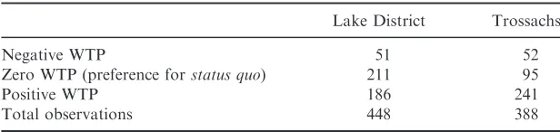
In contingent valuation, despite the fact that many externalities manifest them-selves as costs to some and benefits to others, most studies restrict willingness to pay to being non-negative. In this paper, we investigate the impact of allowing for negative, zero and positive preferences for prospective changes in woodland cover in two UK national parks, the Lake District and the Trossachs. An extended spike model is used to accomplish this. The policy implications of not allowing for negative values in terms of aggregate benefits are also investigated, by comparing the extended spike model with a simple spike making use of only zero and positive bids, and a model which considers positive bids only. We find that ignoring negative values over-states the aggregate benefits of a woodland planting project by up to 44%.
Keywords:Contingent valuation; national parks; negative WTP; spike models.
JEL classifications: D6, Q2.
1. Introduction
Contingent valuation (CV) has been the most widely used stated preference method for environmental valuation. Since the publication of NOAA panel report (Arrow et al., 1993), the use of close-ended choice questions have largely replaced open-ended
1
Nick Hanley is based in the Economics Department, University of Stirling, UK. Sergio Colombo is based in the Agricultural Economics Department, IFAPA, Granada, Spain. E-mail: [email protected] for correspondence. Bengt Kristro¨m is based in the Department of Forest Economics, SLU, Umea, Sweden. Fiona Watson is based at Past Experience, Perthshire, Scotland. We thank the Arts and Humanities Research Board for funding this work through their funding of the AHRB Centre for Environmental History at the Univer-sity of Stirling. Fiona Watson was the Director of this Centre during the empirical parts of this research. We also thank two anonymous referees and the editors for comments on an earlier version of the paper.
questions as the elicitation format to disclose respondents’ willingness to pay (WTP). The dichotomous choice format asks respondents if they are willing or not to pay an offered amount for a specific environmental change, and typically does not allow people who would suffer a loss in utility from the proposed change (such as re-introducing wolves in a national park) to express their negative WTP. Indeed, several authors (e.g. Carson et al., 1992; Batemanet al., 2002) advise the use of dis-tributional assumptions that rule out negative WTP. Similarly, payment card, pay-ment ladder and open-ended CV designs tend to preclude negative values from being expressed. In a referendum-style CV exercise, respondents who do not agree with paying the posted bid may either have a ‘genuine’ zero WTP, have a negative WTP or else can be expressing a protest answer. Whilst respondents who hold a ‘genuine’ zero and those who express a ‘protest’ WTP can be easily identified by using follow-up questions, and the resulting welfare measures corrected (Jorgensen and Syme, 2000), negative WTP statements where allowed are usually considered a sort of protest answer and either excluded from analysis or assigned a value of zero; whilst many survey designs will not even reveal negative WTP responses.
Using valuation approaches which rule out negative WTP may provide biased estimates of welfare change from project or policy execution in circumstances where a significant fraction of the sample actually dislikes the proposed change (in the case of an environmental ‘improvement’). More importantly, when aggregate values are calculated, the exclusion of negative WTP may lead to erroneous conclusions about the net social benefits of the proposed change.
One way of including negative WTP would be to allow respondents to state a positive WTP to prevent the proposed increase in a ‘good’ from going ahead, as suggested by Clinch and Murphy (2001). However, this will not always allow for credible hypothetical markets to be designed, and means that the researcher is required to combine compensating (CS) and equivalent surplus (ES) measures of the same change. An alternative approach is to allow those who would lose out from an increase in the environmental good to express their willingness to accept compensation (WTA) for allowing the changes in question, whilst those who prefer the option state a positive WTP for the same change. However, there are often con-siderable problems in using WTA measures in CV. Such scenarios may lack credi-bility, may be in violation of assumed property right allocations, and can give rise to high levels of protest responses (Hanley et al., 2006). These reasons led the NOAA panel to advise against the use of WTA scenarios in CV, whilst policy-mak-ers have also sought to avoid WTA-based CV designs (Arrow et al., 1993). It might thus be preferable to allow respondents who prefer not to have the environmental change in question to state a positive WTP for a ‘symmetrically opposite’ change: thus, instead of asking WTP for an additional 50 ha of wetland for those who have a positive preference for wetland, one might ask those who have a negative prefer-ence for wetland (for example, because they think of wetlands as breeding grounds for mosquitoes) to state their WTP for a 50-ha reduction in wetland area. This is the approach we follow here.
parks. To respondents who show a preference for a reduction in the forested areas in the park, we ask their maximum WTP for a hypothetical logging project that would result in a reduction in the area of woodland in the park to 20% of the Park’s total area, from a baseline of 30% woodland cover. For respondents who preferred an increase in the forested area, we ask their maximum WTP for a project that would plant broadleaf and mixed woodlands in the park to increase the for-ested area to 40% of the Park’s total area. Making the important assumption that a positive WTP for the felling option is symmetrical to a negative WTP for the planting option, it is possible to combine the two sets of answers in the same log-likelihood function and calculate an overall measure of WTP. We show how this assumption is consistent with a utility function which is linear around the change in question. This treatment of preferences allows, we argue, a much more realistic esti-mate of the population mean WTP value, and of aggregate benefits from woodland change. The welfare estimates obtained from this extended model can then be com-pared with those resulting from a model which includes only positive and zero WTP bids, and a model with positive bids alone.
Section 2 summarises some previous studies where positive and negative WTP values have been modelled. Section 3 describes the study design, whilst section 4 explains the methodological approach followed. Section 5 presents and discusses the results, after which some conclusions are drawn regarding the consequences of extending the modelling framework to negative WTP for aggregate welfare measures and cost–benefit analysis.
2. Previous studies
There have been rather few studies that explicitly account for the existence of nega-tive WTP alongside posinega-tive and zero WTPs, and different approaches have been proposed in the literature to address the problem. Clinch and Murphy (2001) mod-elled positive and negative WTP in a two-stage process. First, they modmod-elled the dichotomous decision for approval⁄disapproval of a project. In a second stage, they modelled the positive WTP for implementing the project (amongst those who approved) and the positive WTP (expressed as the WTP to avoid the project) amongst those who disapproved. In this second stage, they allowed ‘genuine’ zero WTP values. They found, as would be expected, that ignoring welfare losses of the disapprovers produces a significant overestimation of the benefit generated by the proposed project. Note that, in this case, WTP measures to avoid a welfare decrease are combined with WTP measures to gain a welfare increase: in other words, ES and CS measures are treated as commensurate.
An and Ayala (1996) and Werner (1999), using a double-bounded elicitation for-mat, estimated a mixture model where they split people who answered no to both bid questions into two groups: the first made up by people who were assumed to have a WTP included between zero and the minimum bid offered, and the second composed of individuals who were assumed to have a zero WTP. The authors con-cluded that the mixture model was preferred to a conventional double-bounded model and (again) produced lower estimates of mean WTP than the strictly positive WTP model.
the spike model was a better representation of the distribution of stated WTP espe-cially if there is a large number of zero answers. Kristro¨m (1997) also presents an extension of the simple spike model allowing for the inclusion of negative WTP, but did not estimate the model parametrically in the extended spike model case. This is the addition we provide to Kristro¨m’s paper. This approach was also used by Nahuelhaual-Mun˜oz et al.(2004). Our study differs from Nahuelhaual-Mun˜ozet al. (2004) in that they used a WTA measure for allowing an undesirable project to go ahead as an estimate of WTP to prevent the project happening. Given the important conceptual differences that exist between WTP and WTA (Hanemann, 1991), here we ask for WTP bids on both sides of the ‘zero value’ in the WTP distribution.
3. Study design
The study was conducted in two UK national parks, the Lake District National Park, located in north-west England, and Loch Lomond and the Trossachs National Park, located in central Scotland. These areas were chosen as case studies because they have long been important tourist destinations, and have a history of public argument over the extent of woodland cover. The dominance of forestry, especially coniferous plantations, in the Loch Lomond and Trossachs (the Tross-achs) National Park has resulted in a very different landscape from the Lake Dis-trict National Park. Two-thirds of the Trossachs woodlands are coniferous, and woodland is the dominant land use. The forest park contained within the current National Park was one of the earliest such areas to be created (1953) in the UK and was designed to provide recreational opportunities as well as commercial returns. The Trossachs became one of Scotland’s first National Parks in 2002. About 70% of the Scottish population live within one hour’s drive of the park and total tourist numbers were estimated at 2.18 million in 2003 (Loch Lomond and the Trossachs National Park Authority, 2005), whilst around 15,000 people actually live within the park. Many of the Trossachs forests are popularly regarded as poorly designed, and restructuring these forests to accommodate landscape and other concerns is currently a major issue for the Park authority and Forestry Commission. The Lake District was established as a National Park in 1951 and is the largest national park in England. It currently attracts around 12 million visits per annum, whilst around 42,000 people actually live in the Park (Lake District National Park Authority, 2003). Concerns have been expressed over both the establishment and management of woodlands in the Lake District, and the area is often seen as a cul-tural icon of ‘Englishness’. In addition, with the overriding emphasis on biodiver-sity and landscape in both parks, the restoration and expansion of native broadleaved woodland have also been a major focus for debate and action (Whyte, 2002). Both parks support important areas of native woodland of high conservation value.
own homes. We obtained 502 responses in the Lakes and 504 in the Trossachs, divided equally between tourists and local residents.
For the Lake District sample, respondents were told that:
Woodlands and forest cover around one-third of Lake District National Park, and are regarded by some as being important to its special qualities. Currently, this woodland is made up of a mixture of broadleaved woods with species such as oak and ash; and plantations of single evergreen species such as Norway Spruce. Land owners within the park are interested in harvesting the timber, but this would have effects on the landscape. The National Park Authority has to decide how to balance these opposing interests.
They were then told that the Park Authority had to decide what strategy to pur-sue over the next 20 years, and that two broad options existed:
Option 1. If the National Park Authority decides toreduce the forest coverage, this will be carried out by cutting down some of the plantations of evergreens. This would leave about 20% of the National Park still covered in forest.
Option 2. If the National Park Authority decides to increase the forest coverage, this will happen by planting a mix of mainly broadleaved trees such as oak and ash. These new plantings will bring the total wooded area to about 40% of the National Park.
Notice that the nature of the change in forest cover is not identical between the ‘increase’ and ‘reduce’ scenarios. The only realistic scenario in either National Park for new planting is that this new planting would be of native broadleaved trees such as oak and ash. The only realistic scenario for a reduction in tree cover is that this would be achieved by felling of exotic conifer plantations. Respondents then com-pleted a ‘strength and direction of preference’ score card, indicating which of these two scenarios they preferred, and how much they preferred it. This was accom-plished using a nine-point scale of numbered boxes (Figure 1). Ticking a box in the range 1–4 indicated a preference for option 1 above, with lower values implying a stronger preference for less woodland (respondents were offered an explanation as to how to complete this section). Ticking a box numbered 6–9 implied a preference for option 2, with higher values implying a stronger preference for additional wood-land. Ticking box 5 was equivalent to preferring to keep the current situation
(status quo) rather than have either of the two change options. Responses to this question thus yield an ordinal measure of preferences towards future landscape change in the relevant Park.
After expressing their preferences towards the felling or planting project, respon-dents were faced with the CV exercise. Dependent on whether an individual pre-ferred option 1 (reducing forest cover) or option 2 (increasing forest cover), they were asked their maximum WTP to have this option go ahead. Sampling was split between local residents and visitors; for the former group, the bid vehicle was an increase in local taxes; for the latter, it was an increase in car parking fees in the area (these are implemented by the Park Authority). Reasons why such payments were necessary to secure the option were provided; for instance, for option 1 the following text was read to respondents:
Once the trees had been felled, the National Park Authority would need money to restore the landscape, for example by removing tree stumps and encouraging wild flowers and plants to re-grow in the felled areas. Given limited government resources, the Park Authority will need extra funds for the logging project. Money dedicated for this purpose would be collected by increasing local council taxes. This increase would last for 10 years. The only way that the felling project (option 1) could go ahead is if these extra funds were raised.
Those preferring the status quo (by ticking box 5) were not asked their WTP;2 instead, along with those refusing to give any positive payment amount for either option 1 or 2, they were asked why this was in order to distinguish protest bids from genuine zeros (Bateman et al., 2002). The elicitation format used was a pay-ment card showing four amounts. Individuals were asked whether they would defi-nitely pay, probably pay or defidefi-nitely not pay each amount individually.3 This design allows for a degree of uncertainty in how much value respondents place on a given environmental change (Ready et al., 2001). Payment levels were based on a pilot survey in each area of 50 respondents which used an open-ended design. Respondents were reminded that the contribution they made would be dedicated to only this specific project, and that there may be other projects to which he⁄she may be willing to contribute. They were then asked if they were sure about their responses to the four amounts on the payment card, and offered the chance to change any or all responses.
4. Methodology
As pointed out by Clinch and Murphy (2001), it is important to take account of both gainers and losers when valuing an increase in the quality of a public good. Given that individuals typically cannot choose the level of the public good they con-sume, Hicksian CS and ES measures are appropriate for welfare measurement. The CS measures the maximum an individual is WTP for a specified increase in the
2
In retrospect, asking people who preferred the status quo how much they were willing to pay to either stop: (i) an increase in woodland; or (ii) a decrease in woodland would have been useful, although it is not clear which is the more reasonable scenario to select.
3