Robust multi-item newsboy models with a budget constraint
George L. Vairaktarakis
*
Weatherhead School of Management, Department of Operations Research and Operations Management, Case Western Reserve University, 10900 Euclid Avenue, Cleveland, OH 44106-7235, USA
Received 1 April 1998; accepted 6 October 1999 Abstract
In this paper we present robust newsboy models with uncertain demand. The traditional approach to describing uncertainty is by means of probability density functions. In this paper we present an alternative approach using deterministic optimization models. We describe uncertainty using two types of demand scenarios; namely interval and discrete scenarios. For interval demand scenarios we only require a lower and an upper bound for the uncertain demand of each item, while for discrete demand scenarios we require a set of likely demand outcomes for each item. Using the above scenarios to describe demand uncertainty, we develop several minimax regret formulations for the multi-item newsboy problem with a budget constraint. For the problems involving interval demand scenarios, we develop linear time optimal algorithms. We show that the corresponding models with discrete demand scenarios areNP-hard and that they are solvable by dynamic programming. Finally, we extend the above results to the case of mixed scenarios where the demand of some of the items is described by interval scenarios and the demand of the remaining items is described by discrete scenarios. ( 2000 Elsevier Science B.V. All rights reserved.
Keywords: Inventory; Production; Management; EOQ models; Robust optimization
1. Introduction
In this paper we consider the multi-item newsboy model with a budget constraint and demand uncertainty. We present an alternative approach to stochastic optimization by using integer programming models with minimax objectives. We assume that the items of our newsboy model may be of continuous or discrete nature, or a combination of the two. This prompts the introduction of two types of demand scenarios for the items; namely interval and discrete. Before we proceed to further describe our modelling approach as well as to justify our motivation for the structuring of uncertainty via scenarios, we will position this research within the current state of decision theory.
In decision theory there are three di!erent chance environments; namely certainty, riskand uncertainty. Among the three, the certainty and risk environments have received the most attention. In a certainty environment all problem parameters are considered to be accurately known and the objective is to optimize
*Tel.:#1-216-368-5215; fax:#1-216-368-4776. E-mail address:[email protected] (G.L. Vairaktarakis).
a carefully selected performance measure. For the risk environment, parameters are assumed to take on values from carefully selected probability distributions and the objective is to optimize expected system performance.
Certainty and risk environments however, may be inadequate in some cases. For instance, when introduc-ing new products, approximatintroduc-ing their demand may be impossible. Other products exhibit relatively stable
demand, but even then the volume of the demand #uctuates within a small range. These sources of
uncertainty are sometimes captured using risk models. Risk models capture the behavior of uncertain demand with the use of probability distributions. This approach, too, is subject to a few drawbacks. Often, the selected probability distributions only partially capture the behavior of uncertain parameters. Or, the decision situation is of unique nature and hence no historical data are available for the uncertain parameters thus making almost impossible to determine reasonable distributions that capture the behavior of the parameters. In addition, more often than not the incorporation of probability distributions in the risk model make it very di$cult to solve, thus forcing the problem solver to resort to assumptions (such as independence assumptions) that may render the model a mediocre representation of reality. Also, it is customary in risk models to optimize expected system performance. Then, the optimal solution of the risk model provides a guideline for optimizing long-term performance. This may not be in line with the objective of a manager whose survival in the market is based on short-term performance. Several deterministic and stochastic
inventory models are presented in [1}3]. In [4,5], distribution free newsboy problems are considered where
the demand probability distribution is unknown, except for its "rst two moments, and the objective is to
optimize the worst case expected cost over all possible demand distributions with the given "rst two
moments. Similarly, distribution free problems for assemble-to-order, assemble-in-advance, and composite policies are considered in [6]. Additional objective functions for distribution free inventory problems include minimax regret approaches. For instance, in"nite horizon (Q,R) models with backorder costs are considered in [7,8].
A manager who is interested in short-term performance has to exploit the opportunities available to him/her at the time of the decision. This, along with the traditional risk averse attitude of managers, render minimax regret approaches very important in identifying robust solutions, i.e., solutions that perform well for any realization of the uncertain demand parameters. In this paper we present a number of minimax regret formulations for the mutli-item newsvendor problem with a single budget constraint, when the demand distribution is completely unknown. The only assumption made about the demands for individual items is that they may be described with the use of scenarios, or the demand for each item falls within a known lower and upper bound. Under this assumption, in [9] a dynamic programming approach is presented to solve the multi-period newsvendor problem, while in [10] the distribution free newsvendor problem is studied with the objective of minimizing maximum regret.
In this article, our modelling approach incorporates minimax regret objective functions together with the use of scenarios and/or intervals for uncertain demands. Similar approaches have been recently applied in many operations research areas including location theory (see [11,12]), scheduling (see [13,14]), and inventory control (see [15]).
We can now proceed to describe the motivation of the scenario approach for capturing demand uncertainty. First consider items of discrete nature (e.g. magazines, newspapers, tires); for these items we capture demand uncertainty by means of discrete scenarios. A discrete scenario is a collection of possible demand realizations of the item in question. As a result, for every item of discrete nature we associate a scenario, i.e., a set of possible demand realizations. Note that we do not associate probabilities with every possible demand realization; a scenario is just a collection of all possible values for the demand of a particular item. Determining the demand scenario of each item is based on the understanding of the manager on the
sources that a!ect uncertainty (such as market and competitive environment) for each item. In this paper we
a particular item of continuous nature we only need to carefully select a lower and an upper bound for the
demand. Again, all values in the speci"ed interval are considered likely to occur, but there are no
probabilities associated with these values. The upper and lower bounds of interval scenarios are subjectively selected by the decision maker. Demand values that are realized with in"nitesimal probability should only be used if the decision maker is willing to hedge against extremely unlikely scenarios. Else, the range of values in each interval scenario should only contain likely realizations.
In some cases, robust optimization can be used in risk environments where, even though there is distributional knowledge of uncertain input parameters, the intractability of the model makes it
extremely di$cult to derive answers based on stochastic optimization. In this case, one can identify
upper and lower bounds using the 90% quartile or other appropriate percentage. When the distribution of the uncertain parameters is concentrated around the mean, then the 90% quartile can provide relatively
tight and at the same time realistic bounds. Else, the decision maker would have to balance the di!erence
of the lower bound from the upper, with the corresponding quartile of the demand distribution. An example for the feasibility of this approach is provided in [16] who report an application from the apparel industry; for details about this application see [17]. In [16], a scatter diagram is provided of
initial demand forcasts (obtained using experts' opinions) versus season sales for fashion products.
In 24 of the 35 points in this diagram, the experts' opinion is very close to the actual sales, and in the
remaining 11 points the ratio of initial-to-actual sales is no greater than 7. Hence, for all practical purposes, in this application, one can develop reasonable bounds by accounting for about two standard deviations on either side of the mean (in this application the demand distribution for every product is assumed to be normal). Another possible use for the robust optimization approach presented in this article, is for building concensus amongst the various experts. For instance, in [17] the mean demand of each product is taken as the mean of the most likely demand values obtained by seven experts. Rather than obtaining a single value from each expert (i.e., the mean), we can obtain a likely range of values and use
the robust quantity as the mean. Using this approach we can minimize the regret su!ered by all experts
as a group.
In this paper we consider the multi-item newsboy model with a budget constraint. The demand for each of the items is uncertain. Our objective is to make a single period stocking decision prior to realizing the demand for any of the items. At the end of the period we can salvage any unused units at a prespeci"ed price. Stocking decisions for subsequent periods are independent of decisions made in previous periods. Demand uncertainty is captured by means of scenarios that are constructed as described above. The budget constraint may represent the load or volume constraint of a truck, or the space available by the retailer, or the total budget available for the purchase of the items. The deterministic version of this model has appeared in many textbooks (see [1,2]) and it is"rst presented in [18]. The solution of this model (see [19] for a good summary of the known results on deterministic inventory problems with constraints) is based on Lagrangean relaxation. In this paper we consider the robust version of the problem, which is appropriate for the
uncertainty environments mentioned earlier. In the next section we de"ne three di!erent robustness
objectives and formally present the models considered.
2. Problem formulation and basic results
n number of items,
d
i demand for itemi,
n
i(Qi,di) the pro"t function for itemi, for the order quantityQi and demanddi.
The pro"t function for the ith item is given by
n
For a particular item, the classical newsboy approach identi"es the quantity QN that maximizes the
expected pro"t (see [2]). This approach results in
F(QN)"r !c#l
r!s#l,
where F()) is the cumulative distribution function of the probability density function (p.d.f.) f()) of the
demand for that particular item. If the p.d.f. is uniformly distributed in ;[D
1, DM], a straightforward
For our robust formulations we need the following de"nitions. LetDs(i) be the collection of all possible demand realizations for itemi,i"1, 2,2, n. Then, the solution to any of the multi-item problems that will
be stated below must be an-tuple inDs(1)]Ds(2)]2]Ds(n). For discrete demand scenarios we consider three di!erent objective functions. Our "rst objective is calledabsolute robustnessand it is formulated as follows:
where= is our budget constraint. The absolute robustness approach attempts to"nd an-tuple of order
quantities that maximize the worst case pro"t over all possible demand realizations. The second formulation is calledrobust deviation, and is given by
(DR) min
This formulation provides a solution that minimizes over all choices of order quantities the maximum pro"t loss due to demand uncertainty. This is a minimax regret approach where the regret is captured by the di!erencen
i(di,di)!ni(Qi,di); i.e. the pro"t that could be realized if there was no demand uncertainty (in
which case we would orderQ
The third robust formulation is calledrelative robustnessand the corresponding formulation is given by
which minimizes the relative pro"t loss per unit of pro"t that could be made if there was no demand uncertainty. Note that the relative pro"t loss measures the lost pro"t as a percentage of the pro"t that could be made if we knew the actual demand.
In the rest of our analysis it will become clear that the three objectives result to very di!erent choices of order quantities. Similar formulations can be written for the case of interval scenarios. The only di!erence in modeling the continuous case, is that the discrete scenariosDs(i) in models (3)}(5) are replaced by the interval scenarios [D
i, Di] whereDi,Diare the lower and upper bounds for the possible demand realizations of item
i: 1)i)n.
As we will show, some of the above problems are related to the continuous knapsack problem (see [21]):
max +n
This problem can be solved using a property established in [20] which can be stated formally as follows.
Suppose that thenitems are ordered according to nonincreasing order of the ratiow
i/ci(i.e. weight per unit
cost). Then, an optimal solution of the continuous knapsack is given by
f x
solution inO(n) time (and thus avoiding the ordering of thenitems) can be done by identifying the critical
item susing a procedure proposed in [22]. Then, each ratio w
i/ci can be compared against ws/cs which
prompts the assignment of the appropriate value forx
i. Hence, the continuous knapsack problem is solvable
in time linear in the number of variables.
The outline of the rest of the paper is as follows. In Section 3 we consider robust models for a single item. In Section 4 we develop algorithms for the multi-item case with a budget constraint, in the presence of interval demand uncertainty. The case where demand uncertainty is structured by use of discrete scenarios is considered in Section 5. Mixed scenarios where uncertain demand is described by means of discrete scenarios for some items and interval scenarios for others, are considered in Section 6. We close Section 7 with some conclusions.
3. Single-item models
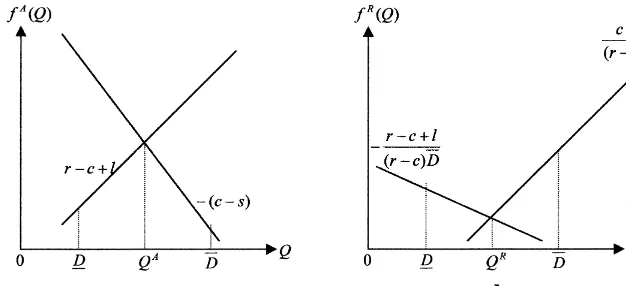
Fig. 1. The order quantities for the absolute, deviation, and relative robust objectives.
variables de"ned in Section 2, e.g.Q
iwill be denoted byQ, etc. Below we obtain the robust order quantity for
each of our three objectives (disregarding the budget constraint).
3.1. Absolute robustness
By observing the pro"t functionn(Q,d), we have that
min
whereQAis the absolute robust-order quantity. For every"xedQ3[D
1 ,DM], the"rst branch of (6) is linear
increasing function ofQ, while the second is linear decreasing; see Fig. 1a.
Hence,QAis in the intersection of the two lines, i.e., the solution ofn(QA, D
1)
"n(QA,DM), which is
QA"(r!s)D1#lDM
r!s#l . (7)
Evidently,QAis a convex combination ofD
1 andDM weighted by (r
!s)/(r!s#l) andl/(r!s#l),
respec-tively. Intuitively,QAhedges against demand uncertainty by charging lost sales on the maximum possible
demandDM (i.e., the termlDM in the numerator), and by chargingr!sunits of lost income for every unit of the
minimum possible volumeD
1.
3.2. Robust deviation
The deviation robust-order quantity is the solution of
min
and it is minimized at the intersectionQDof the two branches; that point is
QD"(c !s)D
1
#(r!c#l)DM
Note that QD is also a convex combination of D
1 and DM, weighted by (c
!s)/(r!s#l) and (r!c#l)/
(r!s#l), respectively. Observe thatQD*QAbecauser!c#l*lwhich indicates that inQD, in addition
to the lost sales l, the lost pro"tr!c is charged against the maximum possible volume DM. As a result,
QDresults to higher service levels and hedges less (as compared with QA) against overestimating actual
demand.
In light of (2) and (8) we have the following corollary.
Corollary 1. The single-item deviation robust-order quantity for the interval demand scenario[D
1, DM],coincides
with the optimal solution of the single-item newsboy model with uniformly distributed demand in [D
1, DM].
turn our attention to the multi-item newsboy model. We start in the next section with demand uncertainty described by interval scenarios.
4. Multiple items and interval demand scenarios
In case that the demand realizations for itemitake values from the interval [D
i, Di], our absolute robust
formulation with a budget constraint becomes
(AR}IS) max
Lemma 1. There exists an optimal solutionMQw
iNni/1forAR}ISsuch thatQ w
i3[Di,QAi],whereQAi is the absolute
robust quantity(7)for itemi.
The proofs of all results are included in the appendix.
In light of this lemma,n
i(Qi,di) can be replaced in AR}IS by (ri!ci#li)Qi!liDi. Then, (11) can be
The optimal solution of (14) maximizes the quantity+
i(ri!ci#li)Qi and therefore AR}IS reduces to
a continuous knapsack problem. We assume that =(+
iciQAi otherwise the trivial solution
Qw
i"QAi, 1)i)n, is optimal. Below we adapt the continuous knapsack procedure of Section 2, for the
formulation AR}IS; we refer to the resulting algorithm for interval demand scenarios, as AID.
4.2. Algorithm AID
1. Index the items so that w
1/c1*w2/c2*2*w2/c2, wherewi"ri!ci#li.
The complexity of AID is O(nlogn), due to the sorting at step 1. However, if the critical element s is
identi"ed"rst (as discussed in Section 2), the sorting can be avoided and the complexity can drop toO(n).
Consider now the deviation robust formulation for interval demand scenarios.
(DR}IS) min
Similar arguments as for AR}IS indicate that there exists an optimal solution for DR}IS whereQw
i)QDi,
whereQDi is the deviation robust quantity given in (8) for itemi. Also, (15) is equivalent to
min
which accepts the same solution as (14). Hence,
Theorem 1. An absolute robust solution MQw
iNni/1 (that solves AR}IS) is also deviation robust (i.e., solves
Finally, consider the relative robustness model with interval demand scenarios
Similar arguments show that AID optimally solves RR}IS if w
i is replaced by wi": (ri!ci#li)/
((r
i!ci)Di). Hence, the item ordering is in nonincreasing order of
f (r
i!ci#li)/ci for the absolute and deviation robust objectives, and
f 1/c
iDi#li/(ci(ri!ci)Di) for the relative robustness objective,
as can be seen by calculating the ratiow
i/ci for each of the objectives. The absolute and deviation robust
objectives favor items with larger ratio of (pro"t#lost sales)/cost. On the other hand, RR}IS favors low-cost
items, whose maximum possible demand is low (due to the termc
iDiin the denominator ofwi/ci), and large
lost sales to pro"t ratiol
i/(ri!ci). A typical example of such environment is a supermarket, where pro"ts are
of the order of 2%, the maximum daily volume for most items is low, and the lost sales costs are signi"cant, since stocking out in a particular item may force the consumer to buy all groceries from a competitor.
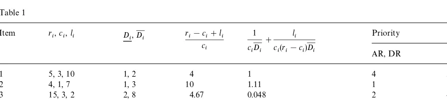
Example. Consider the cost and demand parameters provided below for"ve di!erent items. By identifying the nonincreasing order of the quantities (r
i!ci#li)/ci and 1/ciDi#li/(ci(ri!ci)Di) we indicate in Table
1 which items appear to be given higher priority by each of the three objectives AR, DR and RR for absolute, deviation and relative robustness, respectively.
This example indicates that item 2 receives top priority by all three objectives because it happens to result to a high (pro"t#lost sales)/cost ratio, and at the same time lowD
iand large lost sales to pro"t ratio. Item
1 is favored by the RR objective while its priority is deemed low for the AR and DR objectives. Similar conclusions can be made for the remaining items. As a result, for any budget level, and for every one of the three objectives, our formulations result to ordering the maximum possible number of units starting with high priority items and continuing on with items of lower priority.
5. Discrete demand scenarios
In this section we assume that for each item 1)i)nwe are given a scenarioDs(i) of demand quantities
that may be realized. The number of likely demand outcomes is DDs(i)D. The formulation for the absolute
robust objective is
(AR}DS) max
Qi|Ds(i)
min
di|Ds(i)
n
+
i/1
n
i(Qi,di)
s.t. (12). (17)
In the next section we show that AR}DS is NP-hard.
5.1. NP-hardness result
We will show that AR}DS isNP-hard using a reduction from a well knownNP-hard problem; the
even}odd partition (see [23]).
Input: A collection of positive integersa
i, 1)i)2n, such that+iai"A.
Output:`Yesai!Ma
iN2i/1n can be partitioned into 2 disjoint setsA1,A2such that+ai|Akai"A/2 fork"1, 2
and precisely one ofa
2i, a2i~1belongs toA1, for 1)i)n.
Theorem 2. ProblemAR}DSisNP-complete.
Similar arguments can be used to show the NP-hardness of the deviation and relative robustness
formulations for discrete demand scenarios. In what follows we present optimal solution procedures for these formulations based on dynamic programming.
5.2. Solution procedures
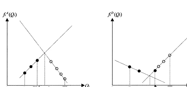
In this section we present dynamic programming optimal algorithms for the case of discrete scenarios and each of the three robust objectives. We"rst consider the absolute robust objective. We assume that the
lowest and highest demand realizations in Ds(i) are D
i and Di, respectively. Then, the function fiA(Qi)"
min
di|Ds(i)ni(Qi,di) is depicted in Fig. 2a.
Observe that Fig. 2a is a discrete version of Fig. 1a precisely because we deal with discrete demand values d
i3Ds(i) rather than interval scenariosdi3[Di, Di] as in Fig. 1a. Note that some of the order quantities in
Fig. 2. The undominated order quantities;1A
Ds(i) are redundant. In Fig. 2a, the redundant quantities are depicted by un"lled circles; and they are the quantities that are greater than the quantity QMAi3Ds(i) that maximizes fAi(Q
i). All these redundant order
quantities have a smaller contribution to the objective function value even though they require a greater expenditure. As a result, they should never be considered in an optimal solution. Hence,
fiA(QMAi)*fA
i (q) ∀q3Ds(i).
Then, the set;A
i of undominated-order quantities consists of those order quantities that are less than or
equal toQM Ai; namely
;A
i ": Mq3Ds(i):q)QMAiN.
Intuitively, the absolute robust performance of the order quantities q3Ds(i)!;A
i are dominated by the
performance ofQMAi becausefiA(QMAi)*fA
i (q) andciQMAi)ciq. Hence, in any optimal solution for AR}DS, only
the order quantities in;A
i need to be considered for itemi. With these observations, AR}DS reduces to
max
which is an integer knapsack problem and can be solved via the following dynamic program:
De"neF
The state space of the above DP isO(n=) due to thenitems and the=units of resource available. In each
iteration, the DP requiresO(max
iDs(i)) e!ort. Letk": maxiDs(i); the total e!ort required by DP is no more
thanO(nk=).
The dynamic programs that solve the deviation and relative robustness formulations for discrete demand scenarios are identical to the one presented above, except for the de"nition of the;A
i's. Fig. 2b depicts by
"lled circles the undominated order quantities for itemiand the deviation robust objective. In general, for the
deviation robust objective the quantityQMDi and the set;D
i are de"ned by
In this section we consider the most general case where some items are of continuous nature while others are of discrete nature. We assume that the demand and order quantities for the former items can be described by an interval scenario as in Section 4 while the latter items can be described by discrete scenarios; in both cases we use the generic notationDsi to denote that scenario. Without loss of generality we can assume that
the items are indexed so that all the items of continuous nature come "rst. Assuming that there are
mcontinuous items, they are followed byn!mitems of discrete nature.
Let us"rst consider the absolute robust formulation AR where the demand scenarios are replaced byDsi. LetMQw
iNni/1be an optimal choice of order quantities for the AR formulation with mixed scenarios. Then, the
portion =
1:"+mi/1ciQ
w
=
2)=!=1 is spent on items of discrete nature. As seen in Sections 4 and 5, the following properties
should hold for an optimal solution for the case of AR with mixed scenarios:
(a) For every item iof discrete nature,Qw
i3;Ai (or;Di,;Ri depending on the objective).
(b) For every itemiof continuous nature,Qw
i3[Di,QAi] (or [Di,QDi], [Di,QRi] depending on the objective).
(c) AID optimally assigns the=
1 units of resource to the continuous items.
(d) DP optimally assigns the=
2 units of resource to the discrete items.
The above observations motivate the development of an optimal algorithm that utilizes AID and DP
along with a search on=
13[+mi/1ciDi,+mi/1ciDi]. The following algorithm provides the main steps of the
proposed procedure.
6.1. Algorithm MIXED
1. Let z
C(=1) be the optimal objective value for the continuous items with a resource of =1 units;
=
13[+mi/1ciDi, +mi/1ciDi].
2. Apply DP on the discrete items with a budget limit of=units.
3. LetZ(=
Step 1 of MIXED can be performed inO(nlogn) time by"rst sorting the items in nonincreasing order of
w
i/ciand then computingzC(=1): =13[+im/1ciDi,+mi/1ciDi] as a piecewise linear increasing function (see
[20]). Step 2 requiresO(nk=) time, while steps 3 and 4 require no more thanO(=) time. Hence, the overall
complexity of MIXED isO(nk=).
Minor adaptation of the above procedure produces an optimal solution to the mixed scenario version of the formulations DR and RR. The only change that needs to be made is that step 4 should be replaced by
Zw
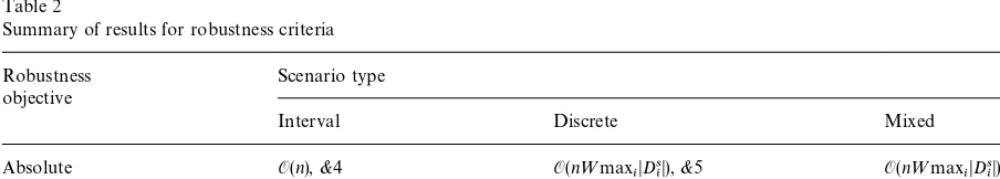
In this article we considered robust newsboy models with a budget constraint. The models are applicable when demand uncertainty can be captured using discrete or interval scenarios. We formulated three minimax
regret objectives and developed e$cient algorithms for nine combinations of objectives and demand
scenarios. Below we summarize the"ndings in Table 2, where we indicate the complexity of the proposed
algorithm for each problem and the section in which it was considered.
Our future research directions include the application of robustness on other inventory models.
Table 2
Acknowledgements
The author would like to thank Professor Panos Kouvelis for bringing this problem to his attention. Also, thanks are due to two anonymous referees whose suggestions greatly improved the presentation and interpretation of our results.
quantityQAi for itemi, the objective of AR}IS does not improve and at the same time a greater portion of the
budget=is consumed. Hence, the optimal quantityQw
i belongs in [Di,QAi]. h
Proof of Theorem 2. Given an instanceMa
iN2i/1n of even}odd partition, consider then-item instance of AR}DS withc
i"1,si"0,li"2,ri"2a2i/(a2i~1), Ds(i)"Ma2i~1,a2iNfor 1)i)n, and="A/2. To see that the
above values result in a well de"ned instance of AR}DS, note that !(c
i!si)"!1 is negative, and
r
i!ci#li"2a2i/(a2i~1)#1'0 which agree with the desired slopes of the lines in Fig. 1a for every itemi. For the above data, and according to (7) we have
QAi" 2a2i~1a2i
Clearly, (A.1) has a solution with objective valueA/2 if and only if there exists a solution to the even-odd
partition problem. This completes the proof of the theorem. h
References
[1] S. Nahmias, Production and Operations Analysis, Irwin, IL, 1989.
[2] E. Silver, R. Peterson, Decision Systems for Inventory Management and Production Planning, 2nd Edition, Wiley, New York, 1985.
[4] G. Gallego, I. Moon, The distribution free newsboy problem: review and extensions, Journal of the Operational Society 44 (8) (1993) 825}834.
[5] I. Moon, G. Gallego, Distribution free procedures for some inventory models, Journal of the Operational Research Society 45 (6) (1994) 651}658.
[6] I. Moon, S. Choi, Distribution free procedures for make to order (MTO), make in advance (MIA), and composite policies, International Journal of Production Economics 42 (1997) 21}28.
[7] G. Gallego, A minimax distribution free procedure for the (Q,R) inventory model, Operations Research Letters 11 (1992) 55}60. [8] G. Gallego, New bounds and heuristics for (Q,R) policies, Management Science 44 (2) (1996) 219}233.
[9] H. Kasugai, T. Kasegai, Characteristics of dynamic maxmin ordering policy, Journal of the Operations Research Society of Japan 3 (1960) 11}26.
[10] H. Kasugai, T. Kasegai, Note on minimax regret ordering policy-static and dynamic solutions and a comparison to maxmin policy, Journal of the Operations Research Society of Japan 3 (1961) 155}169.
[11] P. Kouvelis, G. Vairaktarakis, G. Yu, Robust 1-median location on trees in the presence of demand and transportation cost uncertainty, Research Report, ISE Department, University of Florida, 1994.
[12] G. Vairaktarakis, P. Kouvelis, Incorporating dynamic aspects and uncertainty in 1-median location problems, Naval Research Logistics 46 (1999) 147}168.
[13] R. Daniels, P. Kouvelis, Robust scheduling to hedge against processing time uncertainty in single stage production, Management Science 41 (2) (1995) 363}376.
[14] P. Kouvelis, R. Daniels, G. Vairaktarakis (2000). The 2-machine robust #owshop with processing time uncertainty, IIE Transactions, forthcoming.
[15] G. Yu, Robust economic order quantity models, European Journal of Operational Research 100(3) (1997) 482}493.
[16] M. Fisher, A. Raman, Reducing the cost of demand uncertainty through accurate response to early sales, Operations Research 44 (1) (1996) 87}99.
[17] J. Hammond, A. Raman, Sport Obermeyer, Ltd., Harvard Business School Publishing, Boston, MA, 1996. [18] G. Hadley, T. Whitin, Analysis of Inventory Systems, Prentice-Hall, Englewood Cli!s, NJ, 1963.
[19] M. Rosenblatt, Multi-item inventory systems with budgetary constraint: A comparison between the Lagrangian and the"xed cycle approach, International Journal of Production Research 19 (1981) 331}339.
[20] G.B. Dantzig, Discrete variable extremum problems, Operations Research 5 (1957) 266}277.
[21] S. Martello, P. Toth, Knapsack Problems: Algorithms and Computer Implementations, Wiley, Chichester, England, 1990. [22] E. Balas, E. Zemel, An algorithm for large zero}one knapsack problems, Operations Research 28 (1980) 1130}1154.