ISSN: 2278-4721, Vol. 2, Issue 3 (February 2013), PP 14-26
Www.Researchinventy.Com
Analysis of Energy Spectra and Wave Function of Trigonometric
Poschl-Teller plus Rosen-Morse Non-Central Potential Using
Supersymmetric Quantum Mechanics Approach
Antomi Saregar
1, A.Suparmi
2, C. Cari
3, H.Yuliani
4 1,4(Graduate Student of Physics Department, SebelasMaret University, Indonesia)2,3(Physics Department, SebelasMaret University, Indonesia)
Abstract
:
The Energy Eigenvalues And Eigenfunction Of Trigonometric Poschl-Teller Plus Rosen Morse Non-Central Potential Are Analysis Using Supersymmetric Quantum Mechanics. Trigonometric Poschl-Teller Plus Rosen-Morse Is A Non-Central Shaped Invariance Potential. Recently Developed Supersymmetric In Field Theory Has Been Successfully Employed To Make A Complete Mathematical Analysis Of The Reason Behind Exact Solvability Of Some Non-Central Potentials In A Close Form. Then, By Operating The Lowering Operator We Get The Ground State Wave Function, And The Excited State Wave Functions Are Obtained By Operating Raising Operator Repeatedly. The Energy Eigenvalue Is Expressed In The Closed Form Obtained Using The Shape Invariant PropertiesKeyword:
Supersymmetric method, Non-central potentials, Trigonometric Poschl Teller plus Rosen MorseI.
Introduction
One of the important tasks of quantum mechanic is finding accurate exact solution of Schrödinger equation for a certain potential [1][3]. It is obvious that finding exact solution of SE by the usual and traditional methods is impossible for real physical system, except certain cases such as a system with oscillator harmonic and hydrogen atom[2-5]. Thus, it is inevitable to use new methods to help us solve the real physical system. Among the cases where we have to refuse ordinary methods and seek new methods are in solving SE with non-central potentials. Accordingly, different methods are used to solve SE with non-non-central potentials among which we can name, factorization method [6-9], NU method [8-10] [11,16], supersymmetry (SUSY QM) [11-13], and Romanovsky Polinomials[12] [13].Supersymmetri is, by definition [14][15], a symmetry between fermions and boson. A supersymmetric field theoretical model consists of a set of quantum fields and of a lagrangian for them which exhibit such a symmetry. The Lagrangian determines, through the action priciple, the equations of motion and hence the dynamical behaviour of the particle. Supersymmetry theories describe model worlds of particles, created from the vacuum by the fields, and the interactions between these particles. The supersymmetry manifests itself in the particle spectrum and in stringent relationship between different interaction processes even if these involve particles of different spin and of different statistics.Recently, some authors have investigated on solving Schrödinger equation with physical potentials including Poschl-Teller potential [16,17], Non-central potential [18], Hulthén plus Manning-Rosen potential[19], trigonometric Rosen-Morse potential and Scarf potential[20], Eckart potential Using NU method[21], and trigonometric Poschl-Teller potential plus Rosen Morse by using Romanovsky polinomial [22]. In this paper, we investigate the energy eigenvalues and eigenfunction of trigonometric Poschl-Teller potential plus Rosen Morse non-central potentials using SUSYQM method. The trigonometric Poschl-Teller was used to describe molecular vibrations, while the trigonometric Rosen-Morse potential was used to describe the essential of the QCD quark-gluon dynamics in the regime suited of the asymptotical freedom of the quarks [23-25]. The angular wave functions are visualized using Maple 12.
II.
Review Of Formula For Supersymmetric Quantum Mechanics
2.1. Supersymmetry Quantum Mechanics (SUSY QM)Witten defined the algebra of a supersymmetry quantum system, there are super charge operators
Q
iwhich commute with the HamiltonianH
ss[10]
Q
i,
H
ss
0
with, i = 1, 2, 3, …N (1a)and they obey to algebra
Q
i,
Q
j
ijH
sswith
H
ss is Supersymmetric Hamiltonian. Witten stated that the simplest quantum mechanical system has N=2, it was later shown that the case where N = 1, if it is supersymmetric, it is equivalent to an N = 2 supersymmetric quantum system [7]. In the case where N = 2 it is defined that,
(
)
2
2
1
2 1
1
x
m
p
Q
and
( )
2 2 1
1 2
2 x
m p
Q
(2)here the are the usual Pauli spin matrices, and
x
p
1
is the usual momentum operator. Twocomponents of SUSY Hamiltonian, we shall write
H
ss asH
, are obtained using equation (1b) and (2) given as,
H H
x dx
x d m dx
d m x dx
x d m dx
d m Hss
0 0
) ( ) ( 2 2
0
0 )
( ) ( 2 2
2 2
2 2 2
2 2 2
(3)
with,
) (
2 2
2 2
x V dx
d m
H
with
) ( ' 2 ) ( )
( 2
x m x x
V
(4a)and,
) (
2 2
2 2
x V dx
d m
H with '( )
2 ) ( )
( 2
x m x
x
V
(4b)with and , are defined as supersymmetry partner in the Hamiltonian,
V
(
x
)
andV
(
x
)
are thesupersymmetry partner each other.
Equations (4a) and (4b) are solved by factorizing the Hamiltonian as
A
A
x
H
(
)
, andH
(
x
)
AA
(5)where,
(
)
2
dx
x
d
m
A
and(
)
2
dx
x
d
m
A
(6)with,
A
as raising operator, andA
as lowering operator.2.2. Shape Invariance
Gendenshteın [1]discovered another symmetry which if the supersymmetric system satisfies it will be an exactly solvable system, this symmetry is known as shape invariance. If our potential satisfies shape invariance properties we can readily write down its bound state spectrum, and with the help of the charge operators we can find the bound state wave functions [10,14]. It turned out that all the potentials which were known to be exactly solvable until then have the shape invariance symmetry. If the supersymmetric partner potentials have the same dependence on x but differ in a parameter, in such a way that they are related to each other by a change of that parameter, then they are said to be shape invariant. Gendenshteın stated this condition in this way,
)
(
)
;
(
)
;
(
1 1
x
a
j
V
x
a
j
R
a
jV
(7)with, '( ; )
2 ) ; ( ) ;
( 2
j j
j x a
m a
x a
x
V
(8a)'( ; )
2 ) ; ( ) ;
( 2
j j
j x a
m a
x a
x
V (8b)
where j = 0,1,2,.., and a is a parameter in our original potential whose ground state energy is zero.
)
(
1 j
j
f
a
a
where f is assumed to be an arbitrary function for the time being. The remainderR
(
a
j)
can bedependent on the parametrization variable a but never on x. In this case
V
is said to be shape invariant, and wecan readily find its spectrum, let us take a look at H,
0 0 2
2 2
0 ( ; )
2 dx V x a E
d m E
H
H
(9)
0 0 0
2 0
0 '( ; )
2 ) ; ( )
; ( )
( x a E
m a
x E
a x V x
V
(10)where
V
(
x
)
is the effective potentialV
eff, while
(
x
)
is determined hypothetically from equation (10) basedon the shape of effective potential from the associated system.
By setting
H
H
0 andH
H
1 and by applying equations (7), (8a) and (8b) we get thegeneralized
k
th hamiltonian equation as,
k
i i
k
k V x a R a
dx d m
H 2 1
2 2
) ( )
; ( 2
, with k= 0, 1, 2,… (11)
By applying the characteristic of the Hamiltonian operated to the lowest wave function it is found that
ki
R
a
iE
1 )
(
0
(
)
. So that, in eigen energy spectra of is obtained as,
nk k
n
R
a
E
1 )
(
)
(
(12)Furthermore, we get the total energy spectra from equation (9) as ,
0 ) (
E
E
E
n
n
(13)with as ground state energy of the system.
Based on the characteristics of lowering operator, then the ground state wave function is obtained from equation given as,
0
) (0
A
(14)Meanwhile, the first excited wave function and so forth are obtained by operating raising
operator to the ground state wave function In general,
n
thexcited state wave function is obtained from the nearest lower wave function given as,)
;
(
)
;
(
)
;
(
0 0 ( )1 1) (
a
x
a
x
A
a
x
nn
(15)The explanation above is the simple algebra procedure to construct the hieracy of Hamiltonian. In the next session, the solution of Schrödinger equation will be investigated by using supercharge operator for either one dimension system or three dimension system which is reduced to one dimension system.
III.
Solution of Schrödinger Equation for trigonometric Poschl-Teller potential plus Rosen Morse Non-central potential using Supersymmetry methodSchrödinger equation for trigonometric Poschl-Teller plus Rosen-Morse Non-central potential is the potentials present simulataneusly in the quantum system. This non-central potential is expressed as,
2 2 2
2
2 2 2
cos ) 1 ( sin
) 1 ( 2
/ cot 2 / sin
) 1 ( 2
) ,
( a a bb
mr r
r m
r
V (16)
The three dimensional Schrödinger equation for trigonometric Poschl-Teller plus Rosen-Morse non-central potential is written as,
2
2
2 2 2
2 2 2
sin 1 sin
sin 1 1
2
r r
r r r r m
E
b b a a mr r
r
m
2 2 2 22 2 2
cos ) 1 ( sin
) 1 ( 2 cot
2 / sin
) 1 ( 2
(17)
If equation (17) multiplied by factor ( 2
2 2
mr
), and then the result is solved using separation variable method
since the non-central potential is separable. By setting
(
r
,
,
)
R
(
r
)
P
(
)
(
)
, with
sin ) ( ) ( ) , , ( (
r e H r X r
RP
im
, we obtain,
0 cos
) 1 ( sin
) 1 ( sin
1 sin
sin 1
2 cot 2 sin
) 1 ( 1
2 2
2 2
2
2 2
2 2 2 2
b b a a P
P
E mr r
r R r r R
r
r
(18)
) 1 ( sin 1 sin sin 1 cos ) 1 ( sin ) 1 ( 2 cot 2 sin ) 1 ( 1 2 2 2 2 2 2 2 2 2 2 2 P P b b a a E mr r r R r r R rr (19)
with is constant variabel separable, where
as orbital momentum number.From equation (19) we get radial and angular Schrödinger equation with single variable as following,
2 cot
2 ( 1) sin ) 1 ( 1 2 2 2 2 22
E mr r r R r r R r r
(20)
or equation (20) multiplied by (r2
R
), with
R
(
r
)
r(r), so using symple algebra, we get,
E m X r r rr 2 2
2 2 2 2 2 ) 1 ( cot 2 sin ) 1 ( 1 (21)
and than, for solve radial Schrödinger equation, we use approximation for centrifugal term,
d r
r2 2 0 sin2 1 1
1 for
1
r
, with12
1
0
d
, 2 2m2 E
, we get,
2 2 0 2 2 2 2 2 sin 1 1 ) 1 ( cot 2 sin ) 1 ( 1 r r r dr
(22)
from equation (22) simplied by (
m
2 2
) we get radial Schrödinger equation,
2 2 0 2 2 2 2 2 2 2 2 2 ) 1 ( 2 cot 2 sin ) 1 ( ) 1 ( 22
m d m m r m r r (23)
The angular Schrödinger equation obtained from equation (19) is given as,
) 1 ( sin 1 sin sin 1 cos ) 1 ( sin ) 1 ( 2 2 2 2
2
P P b b a a (24)
and by setting 2
2 2 1 m
we get azimuthal wave function as
,... 2 , 1 , 0 , 2
1
eim m
(25)
and equation (24) becomes,
) 1 ( sin sin sin 1 cos ) 1 ( sin ) 1 ( 2 2 2
2
m P P b b a a (26)
with
m
2as variable separation and we get one dimensional angular Schrödinger equation,H m H b b m a a m d H d
m cos 2 ( ( 1) )
) 1 ( sin ) 1 ( 2 2 4 1 2 2 2 4 1 2 2 2 2 2 (27)
3.1. The solution of Radial Scrodinger Equation for trigonometric Poschl teller potential plus Rosen Morse
Factor R in equation (20) is defined as wave function
, then the Schrödinger equation fortrigonometric Poschl-Teller plus Rosen-Morse potential in radial with the assumption of 2 2
2
'
m can berewritten as follow,
' ) 1 ( 2 cot 2 sin ) 1 ( ) 1 ( 22 2 0
2 2 2 2 2 2 2 d m m r m r
r
(28)
Based on equation (28), the effective potential of radial SE trigonometric Poschl-Teller plus Rosen-Morse is rewritten as,
2 02 2 2 2 ) 1 ( 2 cot 2 sin ) 1 ( ) 1 (
2m m d
V r
r
eff
(29) or,
2 02 2 2 2 ) 1 ( 2 cot 2 sin ) 1 ' ( '
2m m d
V r
r
eff
with 21 4 1
)
1
(
)
1
(
'
By inserting effective potential in equation (30) into equation (10), we obtain
2 0
2
2 2 2
2 ( 1)
2 cot 2 sin ) 1 ' ( ' 2 ) ( ' 2 ) ( d m m x m x r
r
(31)
with
is factorization energy or ground state energy of the system. From equation (31) it is intellectually guessed that superpotential in equation (30) is proposed as,A B r
A
x
)
cot(
)
(
(32)where A and B are indefinite constants that will be calculated. From equation (32), we can determine the value of '(x) and
2(
x
)
, then the result is inserted into equation (31) and we get
2 0
2 2 2 2 2 2 2 2 2 2 ) 1 ( 2 cot 2 sin ) 1 ' ( ' 2 ) ( sin 1 2 ) cot( 2 ) (
sin m m d
A m A B B A A r r r r
r
(33)
By analysing the similar term between left and right hand side in equation (33), we obtain,
r r r r m B m A m A cot 2 ) cot( ; ) ( sin 1 )) 1 ' ( ' ( 2 ) ( sin 1 2 2 2 2 2 2 22
;
and
2 0
2 2 2 2 ) 1 (
2m d
A B
A (34)
From the three equation in equation (34), it is obtained that,
'
2
m
A and ( ' 1)
2
m
A (35a)
2 22m
B (35b)
2 0
2 2
2 2
0 ( ' 1) ( 1)
) 1 ' (
2m d
E
(35c)The value of A and B arechosen by considering that the value of is equal to zero, so,
) 1 ' ( ) cot( ) 1 ' ( 2 ) (
r
m
r (36)
By using equations (6) and (36), we get
) 1 ' ( ) cot( ) 1 ' ( 2 2 ) ( 2
r
m dr d m r dr d m
A (37)
and ) 1 ' ( ) cot( ) 1 ' ( 2 2 ) ( 2
r
m dr d m r dr d m
A (38)
The ground state wave function is obtained from equation (14) and (38) given as,
0 )
(
2 0
r dr d m that gives,
d r a r d r dr) 1 ' ( ) ( ) cot( ) 1 ' ( ) , ( 0 0 0
C r ar r
) 1 ' ( ) sin( ln ) 1 ' ( ) , (
ln 0 0
r a C r r
) 1 ' ( exp ) sin( ) ,
( 0 ( '1)
0
(39)
By using equation (15) we obtain the first excited wave function as,
)
;
(
)
;
(
)
;
(
( ) 10 0 0
) (
1
r
a
A
x
a
r
a
(40)where
a
0
'
a
1
'
1
, ……,a
n
'
n
is the independent parameter to variable “r”. By inserting the
r C
m dr
d m a
r r r
) 2 ' ( exp )
sin( )
1 ' ( ) cot( ) 1 ' ( 2 2
) ;
( 0 ( '2)
) (
1
r C
m
r r
r
) 2 ' ( exp )
sin( )
cos( ) 3 ' 2 ( ) sin( ) 1 ' )( 2 ' (
) 3 ' 2 ( 2
) 1 ' (
(41)
By repeating the step in obtaining equation (41) we get the upper levels of excited wave function as
)
;
(
),
;
(
0) ( 3 0 ) (
2
r
a
x
a
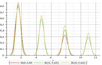
, ... and so on. [image:6.595.72.501.72.135.2]The ground state radial wave functions with various value of the orbital quantum number
n
but with the certain values of potential parameters are shown in Table 1.Tabel 1. ground state radial wave function for trigonometric Poschl-Teller plus Rosen-Morse non-central potential with different orbital quantum number
r
n
a b m
n
'
( )) ' ; ; (
r
n
0 4 2 1 1 0 2 5,6
6,08
08 . 7 08 . 7 ) sin(
r
e r
0 4 2 1 1 1 2
7,6 7,97
97 . 8 97 . 8
) sin(
r
e r
0 4 2 1 1 2 2
9,6 9,9
9 . 10 9 . 10
) sin(
r
e r
The radial wave function of trigonometric Poschl Teller plus Rosen Morse non central potential, it seems only affected by � function that described distant motion or imminent electron from atom core. Polar quantum number , and magnetic quantum number constant, at this point this research was focused on the same electron, therefore, the increasing of disturbance from Rosen Morse non central potential from the value of
[image:6.595.141.456.241.338.2]
, and
'
that getting bigger showed the increasing hyperbolic synus factor of wave function, mathematically, it will be affected to the shift of wave function. The shift that occured can be seen in radial wave function side visualisation on the figure 1. The effect of Poschl-Teller potential to the radial wave function determined by the values of l. The larger is the values of l, the larger is the values of
'
which causes the increase in the wave amplitudes, as shown in Figure 1. The effect is larger for larger r.Figure 1. The ground state radial wave function for trigonometric Poschl-Teller plus Rosen Morse non central potential for different
n
Figure 1. Show that effect of the Poschl Teller non central potential result in the shifting of wave function toward the radial direction �, thus increasing wave amplitudo. The shifting that occured can be seen on the visualisation of wave function radial side on pigure 1, it can be seen that the effect of Poschl Teller non central potential results wave function shift towards radial direction �, but not too significant, then it increasing amplitudo wave. The shift of amplitudo indicates the energy level that getting bigger then electron by way motion that not too far, which indicates the probability of finding bigger electron.By using equations (8a), (8b) and (36), we determine the potential partner which have shape invariant as
2 2
2
2 2
2 2
2 2 2
0 ( ' 1)
) 1 ' ( 2 ) cot( )
( sin
) 1 ' ( ' 2 ) ,
(
m m
m a r
V r
r
(42a)
[image:6.595.217.387.466.575.2]
2 2
2 2 2 2 2 2 2 2
0 ( ' 1)
) 1 ' ( 2 ) cot( ) ( sin ) 2 ' )( 1 ' ( 2 ) , (
m m
m a r V r r (42b)
If we have chosen parameters , …then
obtained by changing
'
into
'
1
in equation (42a) is given as
2 2
2 2 2 2 2 2 2 2
1 ( ' 2)
) 2 ' ( 2 ) cot( ) ( sin ) 2 ' )( 1 ' ( 2 ) , (
m m
m a r V r r (43)
From those two equations (42b) and (43) can be seen that V+ (r,a0) have similar shape with , and by using shape invariance relation in equation (8) we obtain R(a1) as
2
2 2 2 2 2 2 2 2 2 1 0
1 ( ' 2)
) 2 ' ( 2 ) 1 ' ( ) 1 ' ( 2 ) , ( ) , ( ) ( m m a r V a r V a
R (44)
We repeat the step as on the determination of equation (44) by using equations (42a), (42b), and (43),
to obtain and , as,
2 2
2 2 2 2 2 2 2 2
1 ( ' 2)
) 2 ' ( 2 ) cot( ) ( sin ) 3 ' )( 2 ' ( 2 ) , (
m m
m a r V r r
(45a)
2 2
2 2 2 2 2 2 2 2
2 ( ' 3)
) 3 ' ( 2 ) cot( ) ( sin ) 3 ' )( 2 ' ( 2 ) , (
m m
m a r V r r
(45b)
From equ. (45a) and (45b) so obtained,
2
2 2 2 2 2 2 2 2 2 2 1
2 ( ' 3)
) 3 ' ( 2 ) 2 ' ( ) 2 ' ( 2 ) , ( ) , ( ) ( m m a r V a r V a
R (46)
Then, the determination steps on equ. (44) or equ. (46) above are repeated until parameters heading to n, an to
determinate R(an) and finally obtained,
2 2 2 2 2 2 2 2 2 2 1 )( ( ' 1)
) 1 ' ( 2 ) 1 ' ( ) 1 ' ( 2 ) ( r r n k k n n n m m a R E (47)
If equ. (47) and equ. (36c) inserted into equation (13) we obtain the energy spectrum for Rosen Morse system i.e., 0 2 2 2 2 2 0 )
( ( ' 1) ( 1)
) 1 ' (
2m n n d
E E
E r
r n
n
(48)
with,
E
n
'
, and2 1 4 1 ) 1 ( ) 1 ' ( ' '
, so equ. (48) is energy solution of Schrödinger equation for
trigonometric Poschl-Teller plus Rosen Morse non central potential with
n
E m
2 2 2
2 0
2 1 4 1 2 2 1 4 1 2 2 2 2 2 ) 1 ( ) 1 ) 1 ( ) 1 ( ( ) 1 ) 1 ( ) 1 ( ( 2 2
2 E m n n d
m
m r r
2 2 1 4 1 2 0 2 2 1 4 1 2 2 ) 1 ( ) 1 ( ) 1 ( ) 1 ( ) 1 ( 2 r r nr n d n m E (49)Equation (49) showed energy spectra of trigonometric Poschl-Teller plus Rosen Morse non central potential, with,
ℏ : planck constants,
� : elementary particle mass and : constants potential depth, : principe quatum numbers, =1,2,3…
� : radial quantum numbers, �=0,1,2…
: orbital quantum numbers.
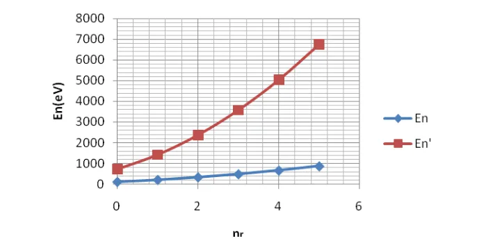
Figure 2. The Energy spectra graph of Rosen Morse potential, with and without the presence of Poschl-Teller potential, with m =1, , μ =1, =2, and
Figure 2. shows that the value of energies affected by quantum orbital number l which depends on the values of Pochl-Teller potential’s parameter.
3.2 The solution of angular Schrödinger equation trigonometric Poschl-Teller plus Rosen Morse non-central potential.
To ease the solution of angular Schrödinger Equation, i.e.,
EH H m( ( 1) )
2 4
1 2
(50)
If equ. (50) incorporated to equ. (28) so angular Schrödinger equation Poschl-Teller plus Rosen Morse non central potential chanced into,
EH H b b m
a a m d
H d
m
2 2
4 1 2 2
2 2 2
cos ) 1 ( sin
) 1 ( 2 2
(51)
Based on equ. (51), effective potential of angular trigonometric Poschl-Teller plus Rosen-Morse non central potential is expressed as,
2
2 4 1 2 2
cos ) 1 ( sin
) 1 ( 2
b b m
a a m
Veff (52)
if, ( 1) 241 '( '1)
a a m
a
a , we get
2
2 2
cos ) 1 ( sin
) 1 ' ( ' 2
b b a
a m
Veff (53)
with
a
'
a
(
a
1
)
m
2
21According to the form of those effective potential equations, then superpotential equation of angular trigonometric Poschl-Teller plus Rosen-Morse non central potential is expressed as,
(
)
A
tan
B
cot
(54)where A and B are indefinite constant that will be calculated. From equ. (54), we determine the value of and , and by using equation (6) we have
2 2 2 2 2 2 2
2 2
cos ) 1 ( sin
) 1 ' ( ' 2 csc sec
2 2
cot
tan a a bb
m B
A m AB B
A (55)
By using in common concept of coefficient between left and right hand side,we obtain
2 2
2
2 2
2 2
2 2
sin 1 ) 1 ' ( ' 2 sin
1 2
; cos
1 )) 1 ( ( 2 cos
1
2
a a m B
m B
b b m A
m
A ;
and E A2 B2 2AB
0
(56)from those third equations on equ. (56) is obtained,
b m A
2
atau ( 1)
2
b
m
(57a) 2 1 2 ) 1 ( 2 ) 1 ' (
2
aa m
m a
m
B
or 2 1 2 ) 1 ( 2 '
2
a a m
m a
m
B (57b)
2 2
0 ( ')
2m b a
E
(57c)A and B value are chosen so that the value of ( ) 0
E is zero. By using eqs. (8a) and (8b) are obtained,
'cot
2 tan 2 ) ( a m b m (58) ) ' ; ( ' 2 ) ' ; ( ) ' ;
( 2 0 0 0 0
0
0 a b
m b
a b
a
V
2 2 2 2 2 ) ' ( 2 cos ) 1 ( sin ) 1 ' ( '
2 m b a
b b a
a
m
(59a)
) ' ; ( ' 2 ) ' ; ( ) ' ;
( 2 0 0 0 0
0
0 a b
m b
a b
a
V
2 2 2 2 2 ) ' ( 2 cos ) 1 ( sin ) 1 ' ( '
2 m b a
b b a
a
m
(59b)
From those two equations (59a) and (59b) is obtained
2 2 2 2 2 1
1 ( ' 2)
2 cos ) 1 ( sin ) 1 ' ( ' 2 ) ' ; (
b a
m b b a a m b a
V
(60)From those two equ. (59b) and (60) can be seen that V+ ( ,a0 ) have the same form with , and by using shape invariance relation on equ. (8), is obtained that
22 2 2 1 1 0 0 1 1
'
2
)
2
'
(
2
)
'
;
(
)
'
;
(
)
'
(
b
a
m
a
b
m
b
a
V
b
a
V
b
a
R
(61)We repeated the step as on determination of equ. (61) with using steps equ. (59), and equ. (60) to obtain
and equations, so obtained,
2 2 2 2 2 1
1 ( ' 2)
2 cos ) 2 )( 1 ( sin ) 2 ' )( 1 ' ( 2 ) ' ; (
b a
m b b a a m b a
V
(62a) 2 2 2 2 2 22 ( ' 4)
2 cos ) 2 )( 1 ( sin ) 2 ' )( 1 ' ( 2 ) ' ; (
b a
m b b a a m b a
V
(62b)
By repeated the step from equ. (62a) to (62b) we often,
22 2 2 2 2 1 1 2
2 ' 2
2 ) 4 ' ( 2 ) ' ; ( ) ' ; ( ) '
( ba
m a b m b a V b a V b a
R (63)
22 2 2
1
1 ' 2 2
2 ) 2 ' ( 2 ) ' ; ( ) ' ; ( ) '
( ba n
m n a b m b a V b a V b a
R n n
n n
n n (64)By repeating the steps in equ. (61) or equ. (63) until parameters heading to n, an to obtain R(an ) as on equ.
(64) and finally it is obtained the parameter that has energy order given as,
2 2 2 2 1 ) ( ' 2 ) 2 ' ( 2 )( b a
m n a b m a R E n k k
n
(65)
If equ. (65) and equ. (57c) are inserted into equation (13) we obtain energy spectrum of Poschl-Teller system so,
22 2 2 2 2 0 ) ( ' 2 ' 2 ) 2 ' (
2m b a n m b a m b a
E E
En n
so 2
2
)
2
'
(
2
m
b
a
n
E
n
(66)with ' 2 12
)
1
(
a
a
m
a
2 21 2 4
1) ( 1) 2
) 1 (
( aa m b n
or a(a1)m2b2n (67)
The angular quantum numbers on equation (67) is used to calculate energy spectrum for potential non central system.
By using equ. (6) and (58) are obtained
( ) 2 2 tan 2 'cot
2 d mb ma
d m d
d m
A (68a)
and
( ) 2 2 tan 2 'cot
2 d mb ma
d m d
d m
A (68b)
By using lowering operator on equ (68b), we calculate the ground state wave function for angular trigonometric Poschl-Teller plus Rosen Morse non-central potential as follows,
0 cot
' 2 tan 2
2 0
mb mad d
m
d b
d a
a d
tan cot
' ) ,
( 0
0
0
21 2
) 1 ( '
0
0
(
,
)
(cos
sin
(cos
sin
b a
b a a mC
C
a
r
(69)Then, by using increasing operator on equ (68a) and basic wave function determinated first level excited wave function,
)
,
(
)
;
(
)
;
(
1) ( 0 0 0
) (
1
a
A
a
a
1
' 1 0) (
1
'
cot
(cos
sin
2
tan
2
2
)
;
(
b aa
m
b
m
d
d
m
a
2 2
'sin cos
) )(cos 1 ' 2 ( ) )(sin 1 2 ( 2
a b
a b
m
(70)
2 2
1
'12
0 ) (
2 tan 'cot (2 3)(sin ) (2 ' 3)(cos cos sin
2 ) ;
(
b a
a b
a b
d d m
a
2 4 2 4 2 2
2
)
(cos
)
)(sin
12
'
12
'
8
(
)
)(sin
3
8
4
(
)
)(cos
3
'
8
'
4
(
2
m
a
a
b
b
ba
a
b
'
sin
cos
b
a (71)To determine the excited wave function above can be done as on determination of first level excited wave function as follows,
)
;
(
),
;
(
0 3( ) 0) (
2
a
a
, and so on. Therefore obtained wave function level that is wanted.
Since , so we get,
sin ) ;
( 0
) (
a
P n
(72)
with
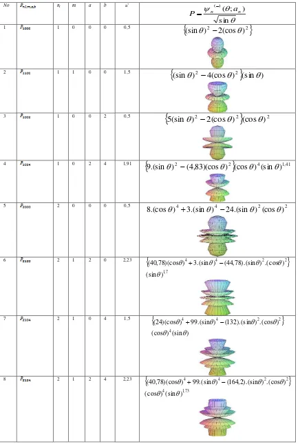
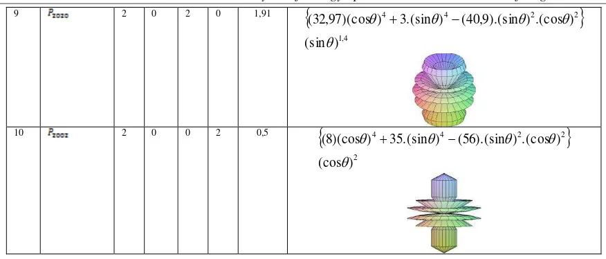
Table 2. Polar wave function of trigonometric Poschl-Teller potential plus Rosen Morse
No nl m a b a’
sin ) ; (
) (
n
n a
P
1 1 0 0 0 0,5
2 2
)
(cos
2
)
(sin
2 1 1 0 0 1,5
)
(sin
)
(cos
4
)
(sin
2
2
3 1 0 0 2 0,5
2 2
2)
(cos
)
(cos
2
)
(sin
5
4 1 0 2 4 1,91
2 2
4 1,41)
(sin
)
(cos
)
)(cos
83
,
4
(
)
.(sin
9
5 2 0 0 0 0,5 4 4 2 2
)
(cos
)
.(sin
24
)
.(sin
3
)
.(cos
8
6 2 1 2 0 2,23
7 , 1
2 2 4
4
) (sin
) .(cos ) ).(sin 78 , 44 ( ) .(sin 3 ) )(cos 78 , 40 (
7 2 1 0 4 1,5
) (sin ) (cos
) .(cos ) ).(sin 132 ( ) .(sin 99 ) )(cos 24 (
4
2 2 4
4
8 2 1 2 4 2,23
73 , 1 4
2 2 4
4
) (sin ) (cos
) .(cos ) ).(sin 2 , 164 ( ) .(sin 99 ) )(cos 78 , 40 (
9 2 0 2 0 1,91
4 , 1
2 2 4
4
) (sin
) .(cos ) ).(sin 9 , 40 ( ) .(sin 3 ) )(cos 97 , 32 (
10 2 0 0 2 0,5
2
2 2 4
4
) (cos
) .(cos ) ).(sin 56 ( ) .(sin 35 ) )(cos 8 (
Table 2. shown the form of polar wave function connected to the angular spin direction electron momentum also describe solid dependent probability on the angular. Generally, polar wave function definition
is same with radial wave function which is describe the probability of electron finding, but both of it have difference on its motion; if radial wave function connected to the far or near of the electron to the nucleus, so
polar wave function is connected to the rotation of the electron to the nucleus.
IV.
Results And Discussion
The radial wave function of trigonometric Poschl Teller plus Rosen Morse non-central potential seems only affected by � function that describe far or near electron motion frrom the atom core. Orbital quantum numbers , , and magnetic quantum numbers constants , on this research is focused on the same electron. Hence to that, the increasing effect of Rosen Morse non central potential of , and ’ value that getting bigger show the increasing hyperbolic synus factor of wave function, mathematically, will be affected to the shift of wave function. The shift that occured can be seen on the visualisation of radial ground state wave function on Figure 1, it shown that trigonometric Poschl Teller potential results on the shift of wave function towards � radial direction, but not too significant, at the same time increase wave amplitudo. The shift of amplitudo indicates the level of energy that getting bigger also electron byway motion that is not too distant, which indicates the probability of bigger electron found.Equation (49), is obtained energy spectra grafic of trigonometric Poschl Teller plus Rosen Morse non central potential, can be seen that value of orbital quantum numbers affected by value, with m, , μ dan constants. The bigger determinate capacity of effect from Poschl Teller potential, at this point, the bigger , Rosen Morse potential will experience the bigger effect from Poschl Teller potential, so that the electrons need higher energy to be on certain layer.On table 2, showed that parameter and influencing wave function. Value of gives exponential factor to the wave function while value increasing sinusoidal factor wave function. At this matter, value of polar quantum number factor ( ) gives influence on the complex fraction of angular function. Parameter which is affected by factor ‘m’value that break down angular function with little angular function, parameter breaks down angular function with big angular function. Figure from table 2, show that there are close and open wave visualisation results. Those results are affected by the existence of sinusoidal factor on the wave function that were used. It can be seen that if synus factor on wave function equation have value, then the resulted wave visualisation is open, and on the contrary.
V.
Conclusion
Based on the describtion, on III and IV point, proved that trigonometric Poschl Teller potential plus Rosen Morse non central potential for group of shape invariance potential can be solved with Supersimmetric method.
VI.
Acknowledgements
Reference
[1] Ballentine, 1999, Quantum mechanics, Simon Fraser University
[2] Gonul.B and Zorba.I, 2000. Phys. Lett. A Vol 269 (2000) 83-88, Supersymmetric Solution of Non-Central Potetials,Department of Engineering Physics, Gaziantep University, Turkey
[3] Gonul. B and Kocak. M, 2005, [arXiv : quant-ph/0409085v3], Systemic Search of Exactly Solvable Non-Central Potentials, Department of Engineering Physics, Gaziantep University, Turkey
[4] C.Y Chen and S. H. Dong,Exactly complete solutions of the Coulomb potential plus a new ring-shaped potential, Phys. Lett. A 335 (2005) 374
[5] H.X. Quan, L. Guang, W.Z. Min, N.L. Bin, and M. Yan, Solving Dirac Equation with New Ring-Shaped Non Spherical Harmonic Oscillator Potential, Com. Theor. Phys. (China) 53 (2010) 242
[6] Infield. L and Hull.TD, Rev. Mod Phys.23 (1951) 21 E. Schrödinger, Proc.R. Irish Acad. A46(1940) 9
[7] M. Combescure, F. Gieresand, and M. Kibler. Are n = 1 and n = 2 supersymmetric quantum mechanics equivalent? Journal of Physics A: Mathematical and General, 37(43):10385–10396, 2004.
[8] Salehi. H, 2011, Aplied Mathematics, Determine the Eigen Function of Schrödinger Equation with Non-Central Potential By Using NU Method, Department of Physics, Shahid Chamran University, Iran
[9] Sadeghi. J and Pourhassan. B, 2008, Electronic Journal of Theoretical Physics, Exact Solution of The Non - Central Modified Kratzer Potential Plus a Ring - Shaped Like Potential By The Factorization Method, Sciences Faculty Department of Physics, Mazandaran University, Iran
[10] Mustafa. M and Kais. M, 2009, [arXiv : math-ph/4206v2], A Vann Diagram for Supersymmetric, Exactly Solvable, Shape Invariant, and Infield-Hull Factorizable Potentials, Department of Physics, Purdue University
[11] Ikhdair. SM and Sever. R, 2007, [arXiv : quant-ph/0702186v1], Polynomial Solution of Non Central Potentials, Department of Physics, Near East University, Turkey
[12] A.Suparmi, C.Cari, J. Handika, C. Yanuarif, H. Marini. 2012. IOSR Journal of Applied Physics. Approximate Solution of Schrodinger equation for Modified Poschl-Teller plus Trigonometric Rosen Morse Non-Central Potentials in Terms of Finite Romanovski Polinomials, Department of Physics, Sebelas Maret Universitas Indonesia
[13] A. Suparmi, 1992, Desertation, Semiclassical SUSY approace in Quantum Mechanics, Department of Physics, Suny at Albany. USA.
[14] Ranabir Dutt, Avinash Khare, and Uday P. Sukhatme. Supersymmetry, shape invariance, and exactly solvable potentials. American Journal of Physics, 56(2):163–168, 1988.
[15] M.F. Sohnius, Introducing Supersymmetry (Cambridge CB3 9EW, NHC: England, 1985) [16] G. Chen, Acta Phys. Sinica, 50 (2001), 1651.
[17] O. Yesiltas, Phys. Scripta, 75 (2007), 41.
[18] F. Yasuk, C. Berkdemir, A. Berkdemir, J. Phys. A: Math. Gen, 38 (2005), 6579-6586.
[19] Meyur, S., Debnath, S., Solution of the Schrödinger equation with Hulthén plus Manning-Rosen potential, Lat. Am. J. Phys. Educ.
3, 300-306 (2009)
[20] S. Meyur, S. Debnath. Eigen spectra for Woods-Saxon plus Rosen-Morse potential , Lat. Am. J. Phys. Educ. Vol. 4, No. 3, Sept. 2010.
[21] H. Gaudarzi, V.Vahidi. Supersymmetric Approach for Eckart Potential Using the NU Method. Adv. Studies Theor. Phys., Vol. 5, 2011, no. 10, 469 – 476, Urmia University, Iran
[22] Dutt. R, Gangopadhyaya. A, and Sukhatme. UP, 1996, [arXiv : hep-th/9611087v1], Non Central Potentials and Spherical Harmonics Using Supersymmetry and Shape Invariance, Department of Physics, Visva-Bharati University, India
[23] A.N. Ikot, L.E.Akpabio and E. J. Uwah, EJTP, 8, 25 (2011) 225-232 [24] D. Agboola, Pram.J.Phys, vol.76,no 6 (2011) 875-885