A study of well-balanced finite volume methods and refinement indicators for the shallow water equations.

(1)

methods and refinement indicators

for the shallow water equations

Sudi Mungkasi

September 2012

A thesis submitted for the degree of Doctor of Philosophy

(2)

(3)

(4)

(5)

The work in this thesis is my own except where otherwise stated.

(6)

(7)

Acknowledgements xi

Publications, Talks, and Awards xiii

Abstract xvii

Abbreviations xix

1 Thesis overview 1

1.1 Motivation . . . 1

1.2 Purpose . . . 2

1.3 Outline and contributions . . . 4

PART I: WELL-BALANCED METHODS 7 2 Well-balanced methods 9 2.1 Introduction . . . 9

2.2 Governing equations and numerical methods . . . 10

2.3 Quantity reconstructions . . . 12

2.4 Numerical tests . . . 15

2.4.1 Steady state: a lake at rest . . . 16

2.4.2 Unsteady state: oscillation on a parabolic bed . . . 18

2.5 Concluding remarks . . . 19

PART II: SOME EXACT SOLUTIONS 23 3 Avalanche involving a dry area 25 3.1 Introduction . . . 25

3.2 Saint-Venant models . . . 26

(8)

viii CONTENTS

3.2.1 Equations in the standard Cartesian coordinate . . . 28

3.2.2 Equations in the topography-linked coordinate . . . 30

3.3 Existing solutions . . . 32

3.4 A new solution . . . 33

4 Avalanche involving a shock 43 4.1 Introduction . . . 43

4.2 A new solution in the standard Cartesian system . . . 45

4.2.1 Derivation of the analytical solution . . . 45

4.2.2 Properties of the analytical solution . . . 51

4.3 A new solution in the topography-linked system . . . 52

5 The Carrier-Greenspan periodic solution 59 5.1 Introduction . . . 59

5.2 Governing equations . . . 61

5.3 Periodic waves on a sloping beach . . . 62

5.3.1 Carrier-Greenspan solution . . . 63

5.3.2 The formulation of Johns . . . 64

5.3.3 Calculating the stage and velocity . . . 65

5.3.4 The Johns approximate solution . . . 67

5.3.5 More accurate approximations . . . 68

5.4 Computational experiments . . . 70

5.4.1 First test case: the Johns prescription is successful . . . . 72

5.4.2 Second test case: the Johns prescription fails . . . 77

5.5 Rate of convergence . . . 82

PART III: INDICATORS FOR ADAPTIVE METHODS 85 6 Numerical entropy production 87 6.1 Introduction . . . 87

6.2 Numerical entropy production in 1D . . . 88

(9)

6.2.2 An alternative numerical entropy scheme . . . 91

6.2.3 Numerical tests . . . 93

6.3 Numerical entropy production in 1.5D . . . 104

6.3.1 Governing equations and numerical schemes . . . 104

6.4 Numerical entropy production in 2D . . . 109

6.4.1 Numerical entropy scheme . . . 109

7 Weak local residuals 117 7.1 Introduction . . . 117

7.2 Weak local residuals of balance laws . . . 118

7.3 Weak local residuals of shallow water equations . . . 120

7.3.1 Well-balancing the weak local residual . . . 121

7.3.2 Wet/dry interface treatment for weak local residuals . . . . 124

7.4 Weak local residuals in adaptive methods . . . 131

7.4.1 A one-dimensional flow with topography . . . 134

7.4.2 A one-dimensional dam break with passive tracer . . . 135

7.4.3 A planar dam break . . . 136

7.4.4 A radial dam break . . . 138

8 Conclusions and future work 143 8.1 Conclusions . . . 143

8.2 Future work . . . 144

A Equations and methods in two dimensions 145 A.1 Integral forms of shallow water equations . . . 145

A.2 Finite volume methods . . . 146

B Data structure for triangulations in i_FEM ₁₄₉ B.1 A newest vertex bisection for refinement . . . 150

B.2 A nodal-wise algorithm for coarsening . . . 150

(10)

x CONTENTS

(11)

The work for this thesis was undertaken at the Department of Mathematics, Mathematical Sciences Institute, The Australian National University (ANU). Here I acknowledge the contribution and support of a number of people, in-stitutions and committees over the years of my candidature.

First and foremost, I sincerely thank my primary supervisor, Stephen Roberts, for his guidance, support, and encouragement. I have learnt a lot from him academically and non-academically. He has been very helpful in supporting me to do research in the directions of my own interests, which make me enjoy my PhD research. He has also been supportive to me in getting funds and travel grants during my PhD studies.

I am very grateful to my co-supervisors, Markus Hegland and Linda Stals. I acknowledge some discussions with Markus on weak local residuals and with Linda on adaptive grid methods.

I am indebted to some lecturers, postdoctoral fellows, staff, colleagues, and friends at the ANU. For some discussions, I thank Christopher Zoppou, Vikram Sunkara, Padarn Wilson, Brendan Harding, Mathew Langford, Shi Bai, Bin Zhou, Jiakun Liu, Srinivasa Subramanya Rao, Kowshik Bettadapura, Yuan Fang, and Chin Foon Khoo. I also thank Bishnu Lamichhane, John Urbas and Paul Leopardi also for some discussions. Kind thanks are due to Jodi Tutty and Annie Bartlett at the ANU Academic Skills and Learning Centre for some suggestions on the writing of this thesis. Thanks also go to Nick Guoth, Warren Yang and Kelly Wicks for technical and administrative support.

I thank my friends from Indonesia in Australia for the friendship, which has made me feel at home. Thanks are due to Robertus Anugerah Purwoko Pu-tro and family, Hendra Gunawan Harno, Teddy Kurniawan, Jack Matsay and family, Supomo Suryo Hudoyo and family, Br Budi Hernawan OFM, and other Indonesian friends during my studies in Australia.

(12)

xii CONTENTS

In my PhD period, I was visiting the Department of Applied Mathematics, the University of Washington, U.S.A. and Institut f¨ur Geometrie und Praktis-che Mathematik, RWTH AaPraktis-chen University, Germany. I thank Professor Ran-dall John LeVeque for his assistance and for some discussions, and Jihwan Kim, Jonathan Varkovitzky and Grady Lemoine at the University of Washington for some discussions. I thank Professor Sebastian Noelle for his assistance and some supervision on part of my work, and K. R. Arun, Guoxian Chen, and Marcel Makowski at RWTH Aachen University for some discussions.

During my PhD candidature, I was supported financially by The Australian National University. I acknowledge and thank the following institutions, organi-sations and committees for funding supports during my PhD candidature.

• The Australian National University for ANU PhD and Tuition

Scholar-ships, ANU Vice Chancellor’s travel grants, ANU Miscellaneous (top-up) Scholarships, and funding support for conferences,

• The Australian Mathematical Society (AustMS) for partial funding for my

presentations in the AustMS conference meetings,

• ANZIAM and CSIRO for partial funding through ANZIAM-CSIRO Student

Support Schemes for my presentations in the Engineering Mathematics and Applications Conference as well as Computational Techniques and Appli-cations Conferences,

• Sanata Dharma University for covering the premium of my Overseas Health

Cover Insurance,

• RWTH Aachen University for partial accommodation support while I

vis-ited Professor Sebastian Noelle,

• The University of Washington for one time in-city travel assistance while I

visited Professor Randall John LeVeque,

• The Committe of the 2012 Gene Golub SIAM Summer School (G2S3) for

the G2S3 travel grant funded by the U.S.A. Naval Postgraduate School for my participation in the summer school.

(13)

The following publications and preprints correspond to the work in this thesis.

• S. Mungkasi and S. G. Roberts, 2010, ”On the best quantity reconstructions

for a well balanced finite volume method used to solve the shallow water wave equations with a wet/dry interface”,ANZIAM Journal (E), 51: C48– C65, Australian Mathematical Society. (Based on the work in Chapter 2.)

http://journal.austms.org.au/ojs/index.php/ANZIAMJ/article/view/2576/1289

• S. Mungkasi and S. G. Roberts, 2011, ”A new analytical solution for

test-ing debris avalanche numerical models”, ANZIAM Journal (E), 52: C349– C363, Australian Mathematical Society. (Based on the work in Chapter 3.)

• S. Mungkasi and S. G. Roberts, 2012, ”Analytical solutions involving shock

waves for testing debris avalanche numerical models”, Pure and Applied Geophysics, 169 (10): 1847–1858, Springer. (Based on the work in Chap-ter 4.)

http://dx.doi.org/10.1007/s00024-011-0449-1

• S. Mungkasi and S. G. Roberts, 2012, ”Approximations of the

Carrier-Greenspan periodic solution to the shallow water wave equations for flows on a sloping beach”, International Journal for Numerical Methods in Flu-ids, 69 (4): 763–780, John Wiley & Sons. (Based on the work in Chapter 5.)

http://dx.doi.org/10.1002/fld.2607

• S. Mungkasi and S. G. Roberts, 2011, ”Numerical entropy production for

shallow water flows”,ANZIAM Journal (E), 52: C1–C17, Australian Math-ematical Society. (Based on part of the work in Chapter 6.)

(14)

xiv CONTENTS

• S. Mungkasi, S. G. Roberts, and S. Noelle, 2012, ”Numerical entropy

pro-duction as a refinement indicator for shallow water equations”, preprint. (Based on part of the work in Chapter 6.)

• S. Mungkasi and S. G. Roberts, 2012, ”Well-balanced computations of weak

local residuals for shallow water equations”,preprint. (Based on part of the work in Chapter 7.)

• S. Mungkasi and S. G. Roberts, 2012, ”Weak local residuals as refinement

indicators for shallow water equations”, preprint. (Based on part of the work in Chapter 7.)

• S. Mungkasi and S. G. Roberts, 2011, ”A finite volume method for

shal-low water fshal-lows on triangular computational grids”, Proceedings of IEEE International Conference on Advanced Computer Science and Information Systems (ICACSIS) 2011, pages 79–84. (Based on the work in Appendix A.)

http://ieeexplore.ieee.org/xpl/freeabs_all.jsp?arnumber=6140781

I have presented some parts of this thesis in talks during my PhD candidature. The talks are as follows.

• ”Well-balanced finite volume methods for shallow water flows involving

wet/dry interface” in the 53rd Australian Mathematical Society Annual Meeting, The University of South Australia, Adelaide, Australia, 28 Sep – 1 Oct 2009

• ”Well-balanced finite volume methods for shallow water flows involving

wet/dry interface” in Engineering Mathematics and Applications Confer-ence 2009, The University of Adelaide, Adelaide, Australia, 6 – 9 Dec 2009

• ”A new analytical solution for testing debris avalanche numerical models in

the standard Cartesian coordinate system” in the 54th Australian Mathe-matical Society Annual Meeting, The University of Queensland, Brisbane, Australia, 27 – 30 Sep 2010

• ”A new analytical solution for testing debris avalanche numerical models”

(15)

• ”Numerical entropy production for shallow water flows” in Computational

Techniques and Applications Conference 2010, The University of New South Wales, Sydney, Australia, 28 Nov – 1 Dec 2010

• ”Approximations of the Carrier-Greenspan periodic solution to the shallow

water wave equations for flows on a sloping beach” in the 55th Australian Mathematical Society Annual Meeting, The University of Wollongong, Wol-longong, Australia, 26 – 29 Sep 2011

• ”A finite volume method for shallow water flows on triangular

computa-tional grids” in the IEEE Internacomputa-tional Conference on Advanced Computer Science and Information Systems (ICACSIS) 2011, Jakarta, Indonesia, 17 – 18 Dec 2011

• ”Some exact solutions to shallow-water-type models and their use as

nu-merical test problems” in a Seminar at IGPM, RWTH Aachen University, Aachen, Germany, 9 February 2012

I received the following awards during my PhD candidature.

• Best paper award in the IEEE International Conference on Advanced

Com-puter Science and Information Systems (ICACSIS) 2011, Jakarta, Indone-sia, 17 – 18 Dec 2011,

• Best presentation award, again in the IEEE International Conference on

Advanced Computer Science and Information Systems (ICACSIS) 2011, Jakarta, Indonesia, 17 – 18 Dec 2011,

• ANU Vice Chancellor’s travel grants to visit Professor Randall John

LeV-eque at the University of Washington, Seattle, U.S.A., 16 Nov–14 Dec 2011 and Professor Sebastian Noelle at RWTH Aachen University, Aachen, Ger-many, 6 Jan – 17 Feb 2012, and

• Travel grant from the U.S.A. Naval Postgraduate School to participate in

(16)

(17)

This thesis studies solutions to the shallow water equations analytically and nu-merically. The study is separated into three parts.

The first part is about well-balanced finite volume methods to solve steady and unsteady state problems. A method is said to be well-balanced if it preserves an unperturbed steady state at the discrete level. We implement hydrostatic reconstructions for the well-balanced methods with respect to the steady state of a lake at rest. Four combinations of quantity reconstructions are tested. Our results indicate an appropriate combination of quantity reconstructions for dealing with steady and unsteady state problems.

The second part presents some new analytical solutions to debris avalanche problems and reviews the implicit Carrier-Greenspan periodic solution for flows on a sloping beach. The analytical solutions to debris avalanche problems are derived using characteristics and a variable transformation technique. The an-alytical solutions are used as benchmarks to test the performance of numerical solutions. For the Carrier-Greenspan periodic solution, we show that the lin-ear approximation of the Carrier-Greenspan periodic solution may result in large errors in some cases. If an explicit approximation of the Carrier-Greenspan pe-riodic solution is needed, higher order approximations should be considered. We propose second order approximations of the Carrier-Greenspan periodic solution and present a way to get higher order approximations.

The third part discusses refinement indicators used in adaptive finite volume methods to detect smooth and nonsmooth regions. In the adaptive finite volume methods, smooth regions are coarsened to reduce the computational costs and nonsmooth regions are refined to get more accurate solutions. We consider the numerical entropy production and weak local residuals as refinement indicators. Regarding the numerical entropy production, our work is the first to implement the numerical entropy production as a refinement indicator into adaptive finite

(18)

xviii CONTENTS

(19)

1D, 1.5D, 2D one dimension, one-and-a-half dimensions, two dimensions

CFL Courant-Friedrichs-Lewy

CG Carrier-Greenspan

CK Constantin-Kurganov

FVM Finite Volume Method(s)

i_FEM _{innovative Finite Element Method}

KKP Karni-Kurganov-Petrova

MHR Mangeney-Heinrich-Roche

NEP Numerical Entropy Production

nNEP normalised Numerical Entropy Production

SI Syst´eme International (International System)

WLR Weak Local Residual(s)

(20)

A study of well-balanced finite volume

methods and refinement indicators

for the shallow water equations

Sudi Mungkasi

September 2012

A thesis submitted for the degree of Doctor of Philosophy

(21)

(22)

Dedicated to my wife, Asti, our daughter, Daniella,

(23)

(24)

Declaration

The work in this thesis is my own except where otherwise stated.

(25)

(26)

Contents

Acknowledgements xi

Publications, Talks, and Awards xiii

Abstract xvii

Abbreviations xix

1 Thesis overview 1

1.1 Motivation . . . 1 1.2 Purpose . . . 2 1.3 Outline and contributions . . . 4

PART I: WELL-BALANCED METHODS 7

2 Well-balanced methods 9

2.1 Introduction . . . 9 2.2 Governing equations and numerical methods . . . 10 2.3 Quantity reconstructions . . . 12 2.4 Numerical tests . . . 15 2.4.1 Steady state: a lake at rest . . . 16 2.4.2 Unsteady state: oscillation on a parabolic bed . . . 18 2.5 Concluding remarks . . . 19

PART II: SOME EXACT SOLUTIONS 23

3 Avalanche involving a dry area 25

3.1 Introduction . . . 25 3.2 Saint-Venant models . . . 26

(27)

3.2.1 Equations in the standard Cartesian coordinate . . . 28 3.2.2 Equations in the topography-linked coordinate . . . 30 3.3 Existing solutions . . . 32 3.4 A new solution . . . 33 3.5 Numerical tests . . . 36 3.6 Concluding remarks . . . 41

4 Avalanche involving a shock 43

4.1 Introduction . . . 43 4.2 A new solution in the standard Cartesian system . . . 45 4.2.1 Derivation of the analytical solution . . . 45 4.2.2 Properties of the analytical solution . . . 51 4.3 A new solution in the topography-linked system . . . 52 4.4 Numerical tests . . . 54 4.5 Concluding remarks . . . 57

5 The Carrier-Greenspan periodic solution 59

5.1 Introduction . . . 59 5.2 Governing equations . . . 61 5.3 Periodic waves on a sloping beach . . . 62 5.3.1 Carrier-Greenspan solution . . . 63 5.3.2 The formulation of Johns . . . 64 5.3.3 Calculating the stage and velocity . . . 65 5.3.4 The Johns approximate solution . . . 67 5.3.5 More accurate approximations . . . 68 5.4 Computational experiments . . . 70 5.4.1 First test case: the Johns prescription is successful . . . . 72 5.4.2 Second test case: the Johns prescription fails . . . 77 5.5 Rate of convergence . . . 82 5.6 Concluding remarks . . . 83

PART III: INDICATORS FOR ADAPTIVE METHODS 85

6 Numerical entropy production 87

(28)

CONTENTS ix

6.2.2 An alternative numerical entropy scheme . . . 91 6.2.3 Numerical tests . . . 93 6.3 Numerical entropy production in 1.5D . . . 104 6.3.1 Governing equations and numerical schemes . . . 104 6.3.2 Numerical tests . . . 105 6.4 Numerical entropy production in 2D . . . 109 6.4.1 Numerical entropy scheme . . . 109 6.4.2 Numerical tests . . . 111 6.5 Concluding remarks . . . 115

7 Weak local residuals 117

7.1 Introduction . . . 117 7.2 Weak local residuals of balance laws . . . 118 7.3 Weak local residuals of shallow water equations . . . 120 7.3.1 Well-balancing the weak local residual . . . 121 7.3.2 Wet/dry interface treatment for weak local residuals . . . . 124 7.3.3 Numerical tests . . . 125 7.4 Weak local residuals in adaptive methods . . . 131 7.4.1 A one-dimensional flow with topography . . . 134 7.4.2 A one-dimensional dam break with passive tracer . . . 135 7.4.3 A planar dam break . . . 136 7.4.4 A radial dam break . . . 138 7.5 Concluding remarks . . . 141

8 Conclusions and future work 143

8.1 Conclusions . . . 143 8.2 Future work . . . 144

A Equations and methods in two dimensions 145

A.1 Integral forms of shallow water equations . . . 145 A.2 Finite volume methods . . . 146

B Data structure for triangulations in iFEM 149

(29)

(30)

Acknowledgements

The work for this thesis was undertaken at the Department of Mathematics, Mathematical Sciences Institute, The Australian National University (ANU). Here I acknowledge the contribution and support of a number of people, in-stitutions and committees over the years of my candidature.

First and foremost, I sincerely thank my primary supervisor, Stephen Roberts, for his guidance, support, and encouragement. I have learnt a lot from him academically and non-academically. He has been very helpful in supporting me to do research in the directions of my own interests, which make me enjoy my PhD research. He has also been supportive to me in getting funds and travel grants during my PhD studies.

I am very grateful to my co-supervisors, Markus Hegland and Linda Stals. I acknowledge some discussions with Markus on weak local residuals and with Linda on adaptive grid methods.

I am indebted to some lecturers, postdoctoral fellows, staff, colleagues, and friends at the ANU. For some discussions, I thank Christopher Zoppou, Vikram Sunkara, Padarn Wilson, Brendan Harding, Mathew Langford, Shi Bai, Bin Zhou, Jiakun Liu, Srinivasa Subramanya Rao, Kowshik Bettadapura, Yuan Fang, and Chin Foon Khoo. I also thank Bishnu Lamichhane, John Urbas and Paul Leopardi also for some discussions. Kind thanks are due to Jodi Tutty and Annie Bartlett at the ANU Academic Skills and Learning Centre for some suggestions on the writing of this thesis. Thanks also go to Nick Guoth, Warren Yang and Kelly Wicks for technical and administrative support.

I thank my friends from Indonesia in Australia for the friendship, which has made me feel at home. Thanks are due to Robertus Anugerah Purwoko Pu-tro and family, Hendra Gunawan Harno, Teddy Kurniawan, Jack Matsay and family, Supomo Suryo Hudoyo and family, Br Budi Hernawan OFM, and other Indonesian friends during my studies in Australia.

(31)

In my PhD period, I was visiting the Department of Applied Mathematics, the University of Washington, U.S.A. and Institut f¨ur Geometrie und Praktis-che Mathematik, RWTH AaPraktis-chen University, Germany. I thank Professor Ran-dall John LeVeque for his assistance and for some discussions, and Jihwan Kim, Jonathan Varkovitzky and Grady Lemoine at the University of Washington for some discussions. I thank Professor Sebastian Noelle for his assistance and some supervision on part of my work, and K. R. Arun, Guoxian Chen, and Marcel Makowski at RWTH Aachen University for some discussions.

During my PhD candidature, I was supported financially by The Australian National University. I acknowledge and thank the following institutions, organi-sations and committees for funding supports during my PhD candidature.

• The Australian National University for ANU PhD and Tuition Scholar-ships, ANU Vice Chancellor’s travel grants, ANU Miscellaneous (top-up) Scholarships, and funding support for conferences,

• The Australian Mathematical Society (AustMS) for partial funding for my presentations in the AustMS conference meetings,

• ANZIAM and CSIRO for partial funding through ANZIAM-CSIRO Student Support Schemes for my presentations in the Engineering Mathematics and Applications Conference as well as Computational Techniques and Appli-cations Conferences,

• Sanata Dharma University for covering the premium of my Overseas Health Cover Insurance,

• RWTH Aachen University for partial accommodation support while I vis-ited Professor Sebastian Noelle,

• The University of Washington for one time in-city travel assistance while I visited Professor Randall John LeVeque,

• The Committe of the 2012 Gene Golub SIAM Summer School (G2S3) for the G2S3 travel grant funded by the U.S.A. Naval Postgraduate School for my participation in the summer school.

(32)

Publications, Talks, and Awards

The following publications and preprints correspond to the work in this thesis.

• S. Mungkasi and S. G. Roberts, 2010, ”On the best quantity reconstructions for a well balanced finite volume method used to solve the shallow water wave equations with a wet/dry interface”,ANZIAM Journal (E), 51: C48– C65, Australian Mathematical Society. (Based on the work in Chapter 2.)

• S. Mungkasi and S. G. Roberts, 2011, ”A new analytical solution for test-ing debris avalanche numerical models”, ANZIAM Journal (E), 52: C349– C363, Australian Mathematical Society. (Based on the work in Chapter 3.)

• S. Mungkasi and S. G. Roberts, 2012, ”Analytical solutions involving shock waves for testing debris avalanche numerical models”, Pure and Applied Geophysics, 169 (10): 1847–1858, Springer. (Based on the work in Chap-ter 4.)

http://dx.doi.org/10.1007/s00024-011-0449-1

• S. Mungkasi and S. G. Roberts, 2012, ”Approximations of the Carrier-Greenspan periodic solution to the shallow water wave equations for flows on a sloping beach”, International Journal for Numerical Methods in Flu-ids, 69 (4): 763–780, John Wiley & Sons. (Based on the work in Chapter 5.)

http://dx.doi.org/10.1002/fld.2607

• S. Mungkasi and S. G. Roberts, 2011, ”Numerical entropy production for shallow water flows”,ANZIAM Journal (E), 52: C1–C17, Australian Math-ematical Society. (Based on part of the work in Chapter 6.)

(33)

• S. Mungkasi, S. G. Roberts, and S. Noelle, 2012, ”Numerical entropy pro-duction as a refinement indicator for shallow water equations”, preprint. (Based on part of the work in Chapter 6.)

• S. Mungkasi and S. G. Roberts, 2012, ”Well-balanced computations of weak local residuals for shallow water equations”,preprint. (Based on part of the work in Chapter 7.)

• S. Mungkasi and S. G. Roberts, 2012, ”Weak local residuals as refinement indicators for shallow water equations”, preprint. (Based on part of the work in Chapter 7.)

• S. Mungkasi and S. G. Roberts, 2011, ”A finite volume method for shal-low water fshal-lows on triangular computational grids”, Proceedings of IEEE International Conference on Advanced Computer Science and Information Systems (ICACSIS) 2011, pages 79–84. (Based on the work in Appendix A.)

http://ieeexplore.ieee.org/xpl/freeabs_all.jsp?arnumber=6140781

I have presented some parts of this thesis in talks during my PhD candidature. The talks are as follows.

• ”Well-balanced finite volume methods for shallow water flows involving wet/dry interface” in the 53rd Australian Mathematical Society Annual Meeting, The University of South Australia, Adelaide, Australia, 28 Sep – 1 Oct 2009

• ”Well-balanced finite volume methods for shallow water flows involving wet/dry interface” in Engineering Mathematics and Applications Confer-ence 2009, The University of Adelaide, Adelaide, Australia, 6 – 9 Dec 2009

• ”A new analytical solution for testing debris avalanche numerical models in the standard Cartesian coordinate system” in the 54th Australian Mathe-matical Society Annual Meeting, The University of Queensland, Brisbane, Australia, 27 – 30 Sep 2010

(34)

CONTENTS xv

• ”Numerical entropy production for shallow water flows” in Computational Techniques and Applications Conference 2010, The University of New South Wales, Sydney, Australia, 28 Nov – 1 Dec 2010

• ”Approximations of the Carrier-Greenspan periodic solution to the shallow water wave equations for flows on a sloping beach” in the 55th Australian Mathematical Society Annual Meeting, The University of Wollongong, Wol-longong, Australia, 26 – 29 Sep 2011

• ”A finite volume method for shallow water flows on triangular computa-tional grids” in the IEEE Internacomputa-tional Conference on Advanced Computer Science and Information Systems (ICACSIS) 2011, Jakarta, Indonesia, 17 – 18 Dec 2011

• ”Some exact solutions to shallow-water-type models and their use as nu-merical test problems” in a Seminar at IGPM, RWTH Aachen University, Aachen, Germany, 9 February 2012

I received the following awards during my PhD candidature.

• Best paper award in the IEEE International Conference on Advanced Com-puter Science and Information Systems (ICACSIS) 2011, Jakarta, Indone-sia, 17 – 18 Dec 2011,

• Best presentation award, again in the IEEE International Conference on Advanced Computer Science and Information Systems (ICACSIS) 2011, Jakarta, Indonesia, 17 – 18 Dec 2011,

• ANU Vice Chancellor’s travel grants to visit Professor Randall John LeV-eque at the University of Washington, Seattle, U.S.A., 16 Nov–14 Dec 2011 and Professor Sebastian Noelle at RWTH Aachen University, Aachen, Ger-many, 6 Jan – 17 Feb 2012, and

(35)

(36)

Abstract

This thesis studies solutions to the shallow water equations analytically and nu-merically. The study is separated into three parts.

The first part is about well-balanced finite volume methods to solve steady and unsteady state problems. A method is said to be well-balanced if it preserves an unperturbed steady state at the discrete level. We implement hydrostatic reconstructions for the well-balanced methods with respect to the steady state of a lake at rest. Four combinations of quantity reconstructions are tested. Our results indicate an appropriate combination of quantity reconstructions for dealing with steady and unsteady state problems.

The second part presents some new analytical solutions to debris avalanche problems and reviews the implicit Carrier-Greenspan periodic solution for flows on a sloping beach. The analytical solutions to debris avalanche problems are derived using characteristics and a variable transformation technique. The an-alytical solutions are used as benchmarks to test the performance of numerical solutions. For the Carrier-Greenspan periodic solution, we show that the lin-ear approximation of the Carrier-Greenspan periodic solution may result in large errors in some cases. If an explicit approximation of the Carrier-Greenspan pe-riodic solution is needed, higher order approximations should be considered. We propose second order approximations of the Carrier-Greenspan periodic solution and present a way to get higher order approximations.

The third part discusses refinement indicators used in adaptive finite volume methods to detect smooth and nonsmooth regions. In the adaptive finite volume methods, smooth regions are coarsened to reduce the computational costs and nonsmooth regions are refined to get more accurate solutions. We consider the numerical entropy production and weak local residuals as refinement indicators. Regarding the numerical entropy production, our work is the first to implement the numerical entropy production as a refinement indicator into adaptive finite

(37)

(38)

Abbreviations

1D, 1.5D, 2D one dimension, one-and-a-half dimensions, two dimensions

CFL Courant-Friedrichs-Lewy

CG Carrier-Greenspan

CK Constantin-Kurganov

FVM Finite Volume Method(s)

iFEM innovative Finite Element Method

KKP Karni-Kurganov-Petrova

MHR Mangeney-Heinrich-Roche

NEP Numerical Entropy Production

nNEP normalised Numerical Entropy Production

SI Syst´eme International (International System)

WLR Weak Local Residual(s)

(39)

(40)

Chapter 1

Thesis overview

In this chapter, we provide the motivation, purpose, outline and contributions of this thesis.

1.1

Motivation

The initial motivation of this research comes from natural disasters caused by water flows, such as the Indian Ocean Boxing Day tsunami in 2004. Water flows can be modelled mathematically. One available model is the shallow water equations. Solving the shallow water equations is useful, as the solution can be used to predict where water will flow, how fast it will flow, how large an area is inundated, and if there is a possible dry region for a route of rescue or escape.

Some authors give the shallow water equations [53, 70] different names, such as, shallow water-wave equations [30] or Saint-Venant models [41] (Saint-Venant systems due to A. J. C. B. de Saint Venant [18]). We use these terms interchange-ably depending on the term used in previous work by other researchers.

Exact analytical solutions to the shallow water equations are not available, ex-cept for specific cases (for example, dam break problems [58, 66], debris avalanche problems [41], and waves on a sloping beach [12]). One way to approximate or solve the shallow water equations in general is by use of numerical methods. In this thesis, we study analytical and numerical solutions to the shallow water equations, so that our contributions can be used in building better simulations of shallow water flows.

A number of numerical methods used to solve the shallow water equations are available in the literature. Some of those numerical methods are finite difference

(41)

methods [42, 67], finite element methods [73], and finite volume methods [7, 39, 40]. In this thesis we choose to use finite volume methods, and do not discuss other classes of methods.

Finite volume methods discretise a given domain into a finite number of cells. In the time evolution, the averaged quantities in each cell are updated by nu-merical fluxes and source terms. In particular, a finite volume method used to solve the shallow water wave equations is essentially defined in terms of the recon-struction of conserved quantities at the interfaces between cells, which are used to calculate fluxes across these interfaces.

Finite volume methods have at least two advantages over the physics of shal-low water waves, and hence, over the accuracy of the numerical methods. First, finite volume methods are based on weak (integral) formulations, so the methods should be able to resolve smooth and nonsmooth (discontinuous) solutions better than other numerical methods, such as finite difference methods which are based on differential formulations. It is well-known that the shallow water equations, which are hyperbolic systems, admit discontinuous solutions even when the initial condition is smooth. Second, the methods can conserve the volumes of mass and momentum, as long as conservative numerical schemes are used. More descrip-tions on finite volume methods can be found in lecture notes and text books, such as those written by LeVeque [39, 40] and Bouchut [6].

Even though finite volume methods have the aforementioned advantages, their ability to resolve the steady state solutions and the accuracy of the resulting numerical solutions at wet/dry interfaces, shocks and contact discontinuities are still an issue [2, 53, 57]. This thesis will present possible ways to deal with this issue.

1.2

Purpose

The aims of this thesis are:

a. to propose implementations of well-balanced finite volume methods used to solve the shallow water equations,

(42)

1.2. PURPOSE 3

c. to develop error indicators for adaptive mesh refinement or coarsening for finite volume methods.

In the first aim, we study well-balanced methods. A method is said to be well-balanced if it preserves an unperturbed steady state at the discrete level. A standard (non-well-balanced) method may lead to spurious oscillations of water, when it is used to simulate the steady state of a lake at rest [53]. A well-balanced finite volume method is intended to give accurate solutions of steady state prob-lems, while it can also solve nonsteady state problems. In this thesis, we study well-balanced methods based on hydrostatic reconstructions originally proposed by Audusse et al. [2]. We test different options for the reconstruction variables, and seek an appropriate choice of reconstruction variables for various situations when solving the shallow water equations using finite volume methods.

In the second aim, we study the debris-avalanche problems using the shal-low water or Saint-Venant approach. We use the term debris-avalanche follow-ing the work of Mangeney et al. [41] in order to get a consistent terminology. Most researchers use the term debris-avalanche in relation to the Savage-Hutter model [60, 61], which is a modified Saint-Venant model [18]. New analytical solutions are derived and they can be used as benchmark solutions to test the performance of finite volume or other numerical methods.

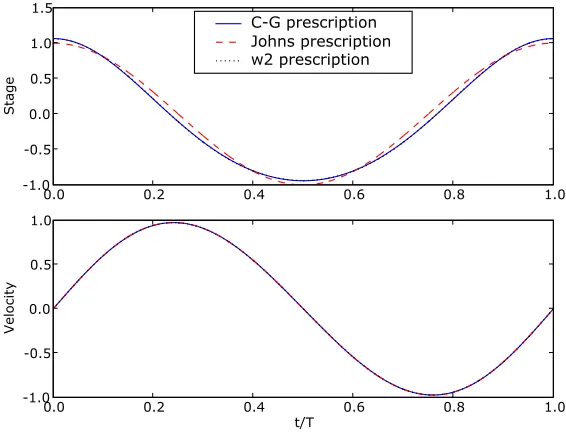
As part of the second aim, some periodic flows on a sloping beach are studied. Analytical and numerical approximations of the flows are compared and discussed. The exact analytical solutions of the periodic flows were originally proposed by Carrier and Greenspan [12] in implicit forms. These exact solutions are often used as benchmark solutions to test the performance of finite volume or other numerical methods. An explicit (closed-form) approximation was introduced by Johns [31] in order to develop a numerical scheme, but we claim that the approximation can lead to large errors in some cases. We derive higher order explicit approximations to get more accurate solutions than that introduced by Johns [31].

(43)

in-dicator for the shallow water equations in particular. Kurganov et al. [32, 33] proposed weak local residuals as smoothness indicators for conservation laws on uniform meshes. We extend the work of Kurganov et al. [32, 33] to balance laws (conservation laws with nonzero source terms) and specifically to the shallow wa-ter equations. We present a way of computing weak local residuals on nonuniform meshes, so that they can be used as smoothness indicators in adaptive-mesh finite volume methods.

1.3

Outline and contributions

This thesis is written in three parts, which correspond to the aims of this thesis. Part I consists of only one chapter, Chapter 2. Part II is constituted of Chapter 3, Chapter 4, and Chapter 5. Part III comprises Chapter 6 and Chapter 7.

The original contributions of this thesis are as follows.

• We give a performance comparison of several combinations of quantity re-constructions and indicate an appropriate choice of combination for a well-balanced method. This is given in Chapter 2. This contribution has been published in ANZIAM Journal [45].

• We derive a new analytical exact solution to the debris avalanche problem involving a dry area, and demonstrate its use in numerical tests. This contribution is covered in Chapter 3, and has been published in ANZIAM Journal [46].

• We derive a new analytical exact solution to the debris avalanche problem involving shock waves, and demonstrate its use in numerical tests. Chap-ter 4 covers this contribution, which has been published inPure and Applied Geophysics journal [48].

• We show that the linear approximation of the Carrier-Greenspan periodic solution can lead to large errors. A new simple formula for the shoreline velocity is presented. We propose second order explicit approximations and present a way to obtain higher order approximations of the exact solution. These contributions are given in Chapter 5, and have been published in

(44)

1.3. OUTLINE AND CONTRIBUTIONS 5

• We formulate numerical entropy production as a refinement indicator for the shallow water equations. We prove properties of numerical entropy schemes relating to the steadiness of a lake at rest and its consistency to the entropy equation on smooth regions. Numerical entropy production is implemented in adaptive methods in one, one-and-a-half, and two dimensions successfully. These contributions are covered in Chapter 6. Some of them have been published in ANZIAM Journal [47].

• We formulate weak local residuals as a refinement indicator for balance laws, and in particular, the shallow water equations. We propose a well-balanced technique to compute weak local residuals of the momentum equation in one dimension. Implementations of weak local residuals in adaptive meth-ods in one, one-and-a-half, and two dimensions are demonstrated. These contributions are given in Chapter 7.

(45)

(46)

PART I:

WELL-BALANCED METHODS

(47)

(48)

Chapter 2

Well-balanced methods

∗

2.1

Introduction

When solving the shallow water wave equations, a robust and accurate numerical method is ideally needed. Such a method should be able to deal with both steady and unsteady state problems. In addition, the error produced by the method should be small on a relatively coarse discretisation of the domain. Recall that this thesis considers finite volume numerical methods.

Constructing a robust and accurate finite volume method is not without dif-ficulties. One well-known difficult task for finite volume methods is wetting and drying processes through wet/dry interfaces. Some authors, such as Bollermann, Kurganov, and Noelle [5], Briganti and Dodd [9], Brufau, Vázquez-Cendón, and Garc´ıa-Navarro [11], Gallardo, Parés, and Castro [24], have attempted to deal with these wetting and drying problems. However, these problems have not been perfectly solved.

In this chapter, we investigate the use of various reconstruction strategies in order to construct a robust and accurate finite volume method that can deal with the wet/dry interface problem and solve both steady and unsteady state problems. We shall make a recommendation on an appropriate choice of reconstruction that leads to an accurate and robust well-balanced method. Note that a numerical method is said to be well-balanced if it preserves an unperturbed steady state at the discrete level.

The remainder of this chapter is organised as follows. We recall the one-dimensional shallow water equations and well-balanced finite volume methods

∗_{The results of this chapter have been published [45].}

(49)

in Section 2.2. In Section 2.3, we provide four combinations of quantity recon-structions. We then test the resulting methods with each combination to solve steady and unsteady state problems, where the simulation results are presented in Section 2.4. Finally, some concluding remarks are drawn in Section 2.5.

2.2

Governing equations and numerical

meth-ods

In this section, we recall the one-dimensional shallow water wave equations and a well-balanced finite volume method.

The conservative form of the one-dimensional shallow water wave equations is

q_t+f(q)x =s, (2.1)

in which the quantity vector q, the flux function f, and the source term s are

q= "

h hu

#

, f= "

hu hu2₊ 1

2gh 2

#

, and s=

" 0

−ghzx

#

. (2.2)

Here, x represents the one-dimensional spatial variable, t represents the time variable, u = u(x, t) denotes the water velocity, h = h(x, t) denotes the water height (depth),z =z(x) denotes the topography (bed elevation), w=h+z is the water stage, and g is the acceleration due to gravity. A mathematical derivation of (2.1) can be found in our previous work [43] or other references [30, 40] on shallow water equations.

An interesting problem arises for the “simple” lake at rest problem. In this case the vertical pressure term (1₂gh2₎

x needs to precisely balance the bed gravity

term−ghzx. For a numerical scheme, the discretisation of these two terms needs

to be carefully undertaken to maintain this balance. A finite volume method is said to bewell-balanced if it preserves this balance, that is if it preserves the lake at rest solution (u = 0, w = constant). Note that there exists a well-balanced method based on moving water, but we do not discuss this type of well-balanced method in this thesis.

(50)

[image:50.595.177.459.99.341.2]

recon-2.2. GOVERNING EQUATIONS AND NUMERICAL METHODS 11

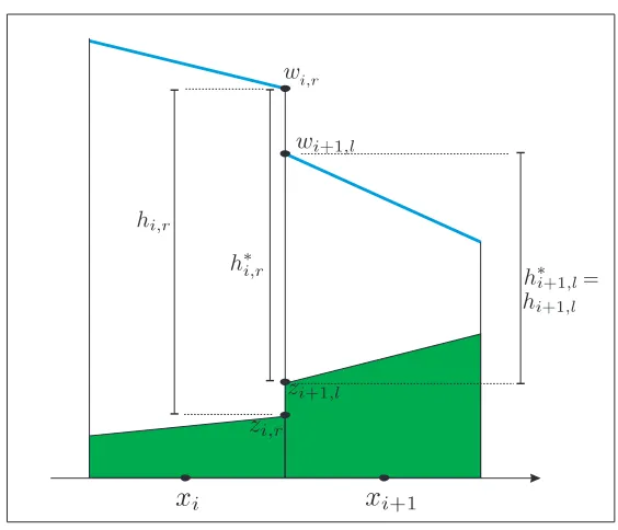
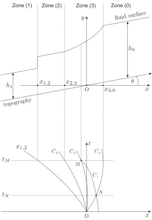
Figure 2.1: An illustration of the hydrostatic reconstruction at an interface between two cells for stagew, heighth, and bed elevationz. In this figure,z∗

i+1 2

=zi+1,l.

struct the values of water depth and bed,hi,r and zi,r on the right edge of theith

cell and hi+1,l and zi+1,l on the left edge of the (i+ 1)th cell.

To obtain a well-balanced scheme, we use the hydrostatic reconstruction that was originally proposed by Audusse et al. [2] for first and second order methods and extended by Noelle et al. [53] for higher order methods. The new recon-structed values of h and z at thei+ 1

2 interface are

z_i∗₊1

2 := max{zi,r, zi+1,l}, (2.3)

h∗_i,r:= max_{0, hi,r+zi,r−z_i∗₊1 2}

, (2.4)

h∗_i₊₁_,l := max_{0, hi+1,l+zi+1,l−z_i∗₊1

2}. (2.5)

An illustration of this spatial setting for the hydrostatic reconstruction is given in Figure 2.1. The values forh∗ _{lead to auxiliary values for the conserved quantities,}

Q∗ = (h∗, h∗u)T _.

A semi-discrete version of our well-balanced finite volume scheme is [2, 53]

∆xi

d

dtQi+F

r₍_Q

i,Qi+1, zi,r, zi+1,l)− Fl(Qi−1,Qi, zi−1,r, zi,l) = S(ij), (2.6)

(51)

at xi+1/2 and xi−1/2, and

Fr₍_Q

i,Qi+1, zi,r, zi+1,l) := F(Q∗i,r,Q∗i+1,l) +Si,r, (2.7)

and

Fl₍_Q

i−1,Qi, zi−1,l, zi,r) := F(Q∗i−1,r,Q∗i,l) +Si,l. (2.8)

Here, Qis the approximation of the vector q, and Fis a conservative numerical flux consistent with the homogeneous shallow water wave equations computed in such a way that the method is stable. In addition,

Si,r :=

"

0

g

2h2i,r− g

2(h∗i,r)2

#

, Si,l :=

"

0

g

2h2i,l− g

2(h∗i,l)2

#

(2.9)

are the corrections due to the water height modification in the hydrostatic recon-struction. Furthermore, the indexj of S(_ij) in equation (2.6) denotes the order of the numerical source term. First and second order numerical source terms are

S(1)_i := "

0 0

#

and S(2)_i := "

0 ghi,l+hi,r

2 (zi,l−zi,r)

#

. (2.10)

The well-balanced finite volume method presented above must be completed by quantity reconstructions used for flux computations, as will be discussed in the next section.

2.3

Quantity reconstructions

In this section, we investigate combinations of reconstruction quantities for finite volume methods used to solve the shallow water equations.

For the one-dimensional shallow water wave equations, we consider five quan-tities, namely: water heighth, bedz, stagew, water velocityu, and momentum p := hu. Reconstructing two elements of the set {h, z, w} together with one element of the set {u, p} is enough to solve the equations in general. We are interested in those reconstructions that involve the reconstruction of stage w as it is the most important quantity in the development of a well-balanced method.

We consider four combinations of reconstruction quantities, namely:

A. stage w and momentum p (where bed z is fixed);

(52)

2.3. QUANTITY RECONSTRUCTIONS 13

C. stage w, water height h, and velocity u;

D. stage w, bedz, and velocity u.

Combination C was used by Audusse et al. [2], and we test the performance of this combination against the other combinations. Combination A, Combination B, and Combination C never result in negative water height, while Combination D results in negative water height at the wet/dry interface if it is applied na¨ıvely. In addition, Combination A and Combination B allow piece-wise continuous linear approximation of the bed topography, while Combination C and Combination D lead to piece-wise discontinuous linear approximation of the bed topography.

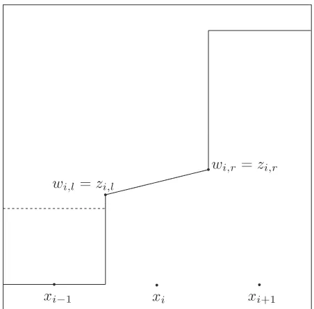
When the second order method is used, Combination D may lead to negative water height if a modification is not made at the wet/dry interface [2]. An occurrence of negative water height is illustrated in Figure 2.2. In order to get a well-balanced method that is physically valid, negative water heights are not allowed. Therefore, we modify the quantity reconstructions around the wet/dry interfaces as follows. Consider the steady state of a lake at rest. We use the minmod limiter [40] for simplicity. Suppose that a wet/dry interface occurs at the ith cell and that zi,r > wi,r. Then we define an auxiliary variableδ =zi,r−wi,r.

In order to maintain conservation, we modify the value of z on both the right and on the left of the ith cell

znew_i,r =wi,r and znewi,l =zi,l+δ . (2.11)

These new values replace the old ones and are used in subsequent computations. Such a modification is shown in Figure 2.3. This modification forces the water height reconstruction to be nonnegative, so that a method using Combination D can be used to solve steady state problems. Unfortunately, a method using Com-bination D with this modification leads to unphysical solutions at wet/dry areas when it is used to solve unsteady state problems, as we will see in Subsection 2.4.2.

(53)

[image:53.595.182.408.122.346.2]

Figure 2.2: An occurrence of negative water height when the minmod limiter is used. Here, the free surface is shown by the dashed line and the water bed by the continuous line.

[image:53.595.182.408.459.682.2]

(54)

2.4. NUMERICAL TESTS 15

2.4

Numerical tests

We provide simulation results in this section. We use Python 2.4 software and adapt the ANUGA package† _{for programming. Steady and unsteady state} prob-lems are considered. The simulations use the second order source term S(2)_i and second order spatial and temporal discretisations.

The numerical setting is as follows. We use the central upwind formulation proposed by Kurganov, Noelle, and Petrova [36] to compute the numerical fluxes. Quantities are measured in Syst´eme International (SI) units, and the acceleration due to gravity is set as g = 9.81 . The minimum water height allowed in the flux computation ishmin = 10−6. The minmod limiter is used for quantity

reconstruc-tion. In the current experiments, each spatial domain is discretised into 400 cells. The Courant-Friedrichs-Lewy (CFL) number used in the simulations is 1.0 .

The discrete L1 _{absolute error}

E = 1 N

N

X

i=1

|q(xi)−Qi| (2.12)

is used to quantify numerical error, whereN is the number of cells, q is the exact quantity function, xi is the centroid of the ith cell, and Qi is the average value

of quantity of the ith cell produced by the numerical method. The L1 _absolute

error is chosen, rather than the relative error, as it applies to both zero velocity and nonzero velocity cases. The relative error of the velocity is not defined for zero velocity.

To compute the velocity based on momentum and height, we proceed as fol-lows. With the momentump=huand the water stagewas conserved quantities, the flux calculation requires the value of velocity uwhere u=p/hand the water depth his calculated by h=w−z. If the water depth approaches zero, the cal-culation of velocity u becomes numerically unreliable and produces unphysically large velocities at wet/dry interfaces. The calculation problems due to small wa-ter depths near a wet/dry inwa-terface can be alleviated by regularising the velocity as described by Roberts et al. [59]. The regularised velocity is defined as

u= p

h+ǫ/h, (2.13)

where ǫ = 10−12 _{is a regularisation parameter that controls the minimal}

magni-tude of the denominator.

(55)

In the following two subsections, numerical results are presented. We consider two representative problems with wet/dry interfaces, namely: a steady “lake at rest with shoreline” and an unsteady “oscillating lake on a parabolic bed”. The first problem has a fixed wet/dry interface, while the second problem has a moving wet/dry interface.

2.4.1

Steady state: a lake at rest

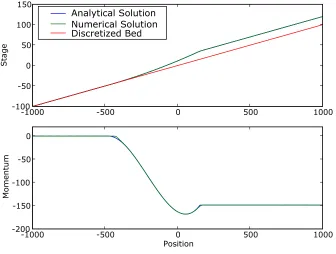
First, we consider the steady state of a lake at rest as follows. Suppose that we have the topography of an artificial lake, with the lake at rest and the stage with a value of w = 4.5 as shown in Figure 2.4. This lake is specifically made so that it has sloping wet/dry interfaces, discontinuous wet/dry interfaces, and discontinuities of the topography. Sloping wet/dry interfaces occur on the left and on the right “ends” of the lake. In addition, discontinuous wet/dry interfaces are found in the middle of the lake due to the existence of an island with very steep shore. This artificial setting is intended to make the problem difficult to solve by numerical methods.

Our experiments show that Methods A and B, which approximate the bedzas a continuous function, fail to be well-balanced. These methods can maintain the well-balanced property at wet/wet interfaces, but fail around wet/dry interfaces. The failure is significant if the wet/dry interface involves large changes in the bed as demonstrated by the island given in our test.

The reason for this failure can be described as follows. When we take the approximation of bedz to be continuous (as in Methods A and B) and the water height h to be nonnegative, we may have a cell with sloping water surface at wet/dry interface as shown in Figure 2.5 so as to maintain the conservation of the water. This leads to a nonzero flux at the interface of that cell, which then induces a nonzero momentum and so the water moves. The motion at wet/dry interface propagates to cells next to it and so on, leading to a lake which is not at rest. Indeed the resulting velocities can be quite large. This type of numerical solution is known as a numerical storm [53].

In contrast, Methods C and D, which approximate the bedz discontinuously, are successful in solving this steady state problem. In our simulations, the results generated by Methods C and D at time t = 2.0 have errors for the momentum and for the velocity on the order of 10−15_{, which is machine accuracy.}

(56)

calcu-2.4. NUMERICAL TESTS 17

Stage

Bed Elevation

0 500 1000 1500 2000

Position 0

1 2 3 4 5 6 7

Stage

[image:56.595.165.474.134.382.2]

Figure 2.4: Cross section for topography of a lake at rest.

(57)

lation is successful in preserving the steady state of a lake at rest if the spatial domain is all wet. However, it may fail in preserving that steady state if the spatial domain contains wet/dry interfaces. Extra care must be taken when re-constructing the quantities in this case.

2.4.2

Unsteady state: oscillation on a parabolic bed

The second test is unsteady state oscillation on a parabolic bed as follows. Con-sider a parabolic canal bed

z = D0 L2x

2_, _(2.14)

whereD0 will denote the maximum equilibrium water depth with an equilibrium

horizontal water surface length of 2L. Let A denote the amplitude of the oscil-lation. We consider initial conditions in this canal, for the water velocity u and stage w given by

u= 0 (2.15)

and

w=D0+

2AD0

L2 [x−A/2]. (2.16)

The solution of this problem consists of the flat water surface moving up one side of the canal, reaching a maximum height and then falling back and then rising on the other side of the canal, and then repeating indefinitely. Therefore, the solution is an oscillation. Following Thacker [71], we find the exact (analytical) solution, in terms of velocity u and stage w, to be

u=−Aωsin(ωt), (2.17)

w=D0 +

2AD0

L2 cos(ωt)

x− A

2 cos(ωt)

, (2.18)

where the angular frequency ω and the period T of oscillation are respectively

ω=

√

2gD0

L and T =

2π

ω . (2.19)

In addition, the shorelines are located at

x=Acos(ωt)_±L . (2.20)

Note that at dry areas we have u= 0 and w=z.

(58)

2.5. CONCLUDING REMARKS 19

Table 2.1: Errors in water heighth, momentumpand velocityuatt=T; and the maximum

absolute velocityumax involved att=T. Method A fails.

Method h error p error u error umax

A - - -

-B 1.26_·10−3 ₁_.₀₀_·₁₀−2 ₂_.₆₀_·₁₀−3 ₀_.₄

C 1.03·10−2 ₈_.₀₈_·₁₀−2 ₁_.₉₄_·₁₀−2 ₀_.₉

D 1.88·10−3 ₁_.₃₇_·₁₀−2 ₂_.₂₅_·₁₀−1 ₇_.₉

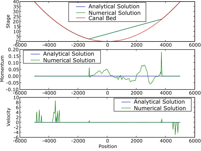
10 , L= 2500 and A=L/2 . The spatial domain to be discretised is the interval [₋2L,2L] .

The error comparison and the maximum absolute velocities umax obtained

at time t = T (where T is the period of oscillation) for the various reconstruc-tion methods are given in Table 2.1. We deem that Method A fails to solve this problem since it requires artificially small time steps relative to the other methods. Methods B and C successfully solve this problem. Method B results in the smallest error (but recall that Method B fails to solve the steady state problem as discussed in Subsection 2.4.1). Figure 2.6 shows the numerical results for Method C at time t =T , and Figure 2.7 is a magnification of Figure 2.6 at cells around wet/dry interface on the interval [3500,3850] . Note that Method D leads to unphysical velocity in some of the dry areas as Figure 2.8 illustrates. Therefore, Method C, which is a well-balanced method with reconstruction on stagew, water heighth, and velocityu, performs better than the other methods in general.

2.5

Concluding remarks

We find that the well-balanced finite volume scheme combined with quantity re-constructions based on stage, height, and velocity has been found to be more robust and accurate than the same scheme combined with quantity reconstruc-tions based on either:

• stage and momentum (where bed is fixed);

• stage and velocity (where bed is fixed); or

(59)

Analytical Solution Numerical Solution Canal Bed

-60000 -4000 -2000 0 2000 4000 6000

5 10 15 20 25 30 35 40 Stage Analytical Solution Numerical Solution

-6000 -4000 -2000 0 2000 4000 6000

-0.4 -0.3 -0.2 -0.1 0.0 0.1 0.2 0.3 0.4 Momentum Analytical Solution Numerical Solution

-6000 -4000 -2000 0 2000 4000 6000

Position -0.4 -0.2 0.0 0.2 0.4 0.6 0.8 1.0 Velocity

Figure 2.6: Simulation results at timet=T using Method C.

3500 3550 3600 3650 3700 3750 3800 3850

Position 20.0 20.5 21.0 21.5 22.0 22.5 23.0 23.5 24.0 Stage

(60)

2.5. CONCLUDING REMARKS 21

-60000 -4000 -2000 0 2000 4000 6000

5 10 15 20 25 30 35 40

Stage

Analytical Solution Numerical Solution

-6000 -4000 -2000 0 2000 4000 6000

-0.10 -0.05 0.00 0.05 0.10 0.15 0.20

Momentum

Analytical Solution Numerical Solution

-6000 -4000 -2000 0 2000 4000 6000

Position -6

-4 -2 0 2 4 6 8 10

[image:60.595.151.474.130.372.2]

Velocity

Figure 2.8: Simulation results at timet=T using Method D. Unphysical velocity occurs at

dry areas.

We note that when the velocity is zero, the momentum is zero. This means that stage and height are the appropriate choice for variable reconstructions to get a well-balanced method.

The discussion in this chapter was limited in one dimension. Many parameters are involved in our numerical simulations, such as the CFL number, the minimum water height allowed in the flux computation, velocity regularisation, and the slope limiter. We have only taken specific values for each of these parameters and used the standard minmod limiter.

(61)

(62)

PART II:

SOME EXACT SOLUTIONS

(63)

(64)

Chapter 3

Avalanche involving a dry area

∗

3.1

Introduction

Avalanche problems have been studied using the Saint-Venant approach (shallow water wave equations) by a number of researchers [41, 46, 52, 65, 66] on a planar topography. The planar topography makes avalanche models simpler than models based on arbitrary topography. Indeed, we limit our discussion in this chapter to problems with planar topography. Readers interested in shallow water models for arbitrary topography are referred to other work, such as that of Bouchut and Westdickenberg [8] and the references therein. In addition, those interested in solving avalanche problems using a modified Saint-Venant model called the Savage-Hutter model [60, 61] are referred to the work of Tai et al. [69] and the references therein.

Some research on dam break and debris avalanche problems using the Saint-Venant model is summarised as follows. Ritter [58] and Stoker [65, 66] solved the so called “dam break” problem for the case with horizontal topography. Man-geney et al. [41] derived an analytical solution to the debris avalanche problem in a topography-linked coordinate system involving a dry area, where the wall separating quiescent wet and dry areas initially is not vertical, but orthogonal to the topography. The dam break and debris avalanche problems were solved by employing the characteristics of the Saint-Venant model.

Because a nonvertical dam is not very similar to some real-world scenarios [1], we shall consider a modified problem having a vertical wall initially and develop its solution in the standard Cartesian coordinate system. That is, in this chapter

∗_{The results of this chapter have been published [46]}

(65)

we derive an analytical solution to a debris avalanche problem having initial vertical wall in the standard Cartesian coordinate system. Characteristics and a transformation technique are used to obtain the analytical solution.

The analytical solution, which we shall derive, to a debris avalanche problem is based on the Saint-Venant approach. Using the Saint-Venant approach implies that debris is treated as a depth-averaged fluid. We use this analytical solution as a benchmark to assess two finite volume methods applied to the debris avalanche problem. The considered debris avalanche problem is a simplification of real world scenarios on the avalanches of debris, such as snow, sands, rocks, as well as landslides. In other words, our work can be an aid in simulations of these real world scenarios.

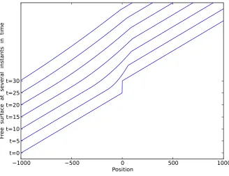
Three problems are considered. The first is the dam break problem in the stan-dard Cartesian coordinate system having initial condition shown in Figure 3.1(a). This problem has been solved by Ritter [58]. The second is the debris avalanche problem in the topography-linked coordinate system having initial condition il-lustrated in Figure 3.1(b). Mangeney et al. [41] have proposed a solution to this problem. The third is the debris avalanche problem in the standard Cartesian coordinate system having initial condition shown in Figure 3.1(c). This third problem represents a modified version of the first and second problems, and is the one we solve in this chapter.

The rest of this chapter is structured as follows. We review the Saint-Venant models involving a Coulomb-type friction in Section 3.2. In Section 3.3, we recall the existing solutions of Ritter [58] and Mangeney, Heinrich, and Roche [41]. Section 3.4 provides a new analytical solution to the modified debris avalanche problem. We implement the new analytical solution to test the performance of finite volume methods and present the numerical results in Section 3.5. Finally, Section 3.6 concludes this chapter with some remarks about the new solution.

3.2

Saint-Venant models

In this section, we review the Saint-Venant model in the standard Cartesian co-ordinate system and the Saint-Venant model in the topography-linked coco-ordinate system. In the previous chapter, derivatives of functions were denoted by short-hand notations like ()x and ()t. Note that here we use the Leibniz notations, like

∂ ∂x and

∂

(66)

3.2. SAINT-VENANT MODELS 27

(a)

(b)

(c)

Figure 3.1: Initial conditions of three considered problems: (a) A dam break problem in

(67)

section.

3.2.1

Equations in the standard Cartesian coordinate

Recall that in the standard Cartesian coordinate system, the mass and momentum equations governing the fluid motion are

∂h ∂t +

∂(hu)

∂x = 0, (3.1)

∂(hu)

∂t +

∂ hu2 ₊1 2gh2

∂x =−gh

dz

dx +hF . (3.2) These two equations are called the Saint-Venant model or the shallow water equations in the standard Cartesian coordinate system. Here, x represents the coordinate in one-dimensional space, t represents the time variable, u = u(x, t) denotes the fluid velocity, h = h(x, t) denotes the fluid height, z = z(x) is the topography, and g is the acceleration due to gravity. In addition, F is a factor representing the Coulomb-type friction defined as

F =−g cos2θ tanδ sgnu (3.3)

in the standard Cartesian coordinate system. This Coulomb-type friction is adapted from the one used by Mangeney et al. [41]. For further reference, we use the notations δ for representing the dynamic friction angle, θ for the angle between the topography (bed elevation) and the horizontal line, and w for the quantity h+z called the stage. For our reference, the values tanδ and tanθ are called the friction slope and bed slope respectively. Note that in the standard Cartesian coordinate system, we limit our discussion to the problems having bed topography z(x) with property dz/dx= tanθ, where θ is constant.

Following Mangeney et al. [41], we limit our discussion to the case when the friction slope is not larger than the bed slope, that is, tanδ ≤ tanθ. With this limitation, after the separating wall is broken, we assume that the fluid motion never stops. Consequently, the Coulomb-type friction (3.3) can be simplified to

F =g cos2_θ _tan_δ _(3.4)

(68)

3.2. SAINT-VENANT MODELS 29

Taking equation (3.1) into account, we can rewrite equation (3.2) as

∂u ∂t +u

∂u ∂x =−g

∂h

∂x −gtanθ+F . (3.5) Introducing a “wave speed”† _{defined as}

c=pgh , (3.6)

and replacing h by c, we can rewrite equations (3.1) and (3.5) as

2∂c ∂t + 2u

∂c ∂x +c

∂u

∂x = 0, (3.7)

∂u ∂t +u

∂u ∂x + 2c

∂c

∂x +gtanθ−F = 0. (3.8) An addition of equation (3.7) to equation (3.8) and subtraction of equation (3.7) from equation (3.8) result in

∂

∂t+ (u+c) ∂ ∂x

·(u+ 2c₋mt) = 0, (3.9)

∂

∂t + (u−c) ∂ ∂x

·(u₋2c₋mt) = 0, (3.10)

respectively, where

m=−gtanθ+F . (3.11)

Note that this value ofmis assumed to be the horizontal acceleration of a particle sliding down an inclined topography [21, 46].

In other words, equations (3.1) and (3.2) are equivalent to the characteristic relations

C+:

dx

dt =u+c , (3.12)

C₋ : dx

dt =u−c , (3.13) in which

u+ 2c−mt=k+ = constant along each curve C+, (3.14)

u₋2c₋mt=k₋ = constant along each curve C₋, (3.15)

where m = −gtanθ+F and c = √gh, and k_± are usually called the Riemann invariants.

†_{Following Stoker [66], we prefer to call}_c_{the wave speed (instead of the wave velocity), as}

(69)

3.2.2

Equations in the topography-linked coordinate

In the topography-linked coordinate system, the Saint-Venant model written in the conservative form with a flat topography is

∂˜h ∂t +

∂˜hu˜

∂x˜ = 0, (3.16)

∂˜hu˜

∂t +

∂˜hu˜2₊1 2gh˜

2_cos_θ

∂x˜ =−˜h

gsinθ−F˜. (3.17)

Equations (3.16) and (3.17) are the equation of mass and that of momentum respectively. Here, ˜x represents the coordinate in one-dimensional space,t repre-sents the time variable, ˜u= ˜u(˜x, t) denotes the fluid velocity, ˜h= ˜h(˜x, t) denotes the fluid height, θ is the angle between the topography (bed elevation) and the horizontal line, andg is the acceleration due to gravity. In addition, ˜F is a factor representing the Coulomb-type friction, given by

˜

F =−g cosθ tanδ sgn ˜u (3.18)

in this topography-linked coordinate system. Recall that we use the notation δ for representing the dynamic friction angle, and the values tanδand tanθare the friction slope and bed slope respectively.

Again, following Mangeney et al. [41], we limit our discussion to the case when tanδ_≤tanθ, so the Coulomb-type friction is defined by

˜

F =g cosθ tanδ (3.19)

for the debris avalanche problem in the topography-linked coordinate system for time t > 0 . We use tilde ˜ notation attached in the quantity variables for those variables corresponding to the problem in the topography-linked coordinate system, and the standard quantity variables (without tilde ˜ notation) are used for variables corresponding to the problem in the standard Cartesian coordinate system.

Taking equation (3.16) into account, we can rewrite equation (3.17) as‡

∂u˜ ∂t + ˜u

∂u˜

∂x˜ =−gcosθ ∂h˜

∂x˜−gsinθ+ ˜F . (3.20)

‡_{Equations (1) and (2) in the paper of Mangeney et al. [41] were called “mass and momentum}

(70)

3.2. SAINT-VENANT MODELS 31

Introducing a “wave speed” defined as

˜ c=

q

gh˜cosθ , (3.21)

Mangeney et al. [41] showed that equations (3.16) and (3.20) can be rewritten as

2∂c˜ ∂t + 2˜u

∂c˜ ∂x˜ + ˜c

∂u˜

∂x˜ = 0, (3.22) ∂u˜

∂t + ˜u ∂u˜ ∂x˜ + 2˜c

∂˜c

∂x˜+gsinθ−F˜ = 0. (3.23) The value of ˜c is the wave speed relative to the fluid velocity ˜u. An addition of (3.22) to (3.23) and subtraction of (3.22) from (3.23) result in

∂

∂t+ (˜u+ ˜c) ∂ ∂x˜

·(˜u+ 2˜c₋mt˜ ) = 0, (3.24)

∂

∂t + (˜u−c˜) ∂ ∂x˜

·(˜u−2˜c−mt˜ ) = 0, (3.25)

respectively, where

˜

m=₋gsinθ+ ˜F . (3.26)

In other words, equations (3.16) and (3.17) are equivalent to the characteristic relations

˜ C+:

dx˜