X to Write a PhD Thesis

(1)

Version 1.3

Nicola L. C. Talbot

Dickimaw Books

www.dickimaw-books.com

(2)

Permission is granted to copy, distribute and/or modify this document under the terms of the GNU Free Documentation License, Version 1.2 or any later version published by the Free Software Foundation; with no In-variant Sections, no Front-Cover Texts, and one Back-Cover Text: “If you choose to buy a copy of this book, Dickimaw Books asks for your support through buying the Dickimaw Books edition to help cover costs.” A copy of the license is included in the section entitled “GNU Free Documentation License”.

(3)

Abstract

vi

1

Introdu

ction

1

1.1 Building Your Document . . . 3

1.1.1 LaTeXmk. . . 5

1.1.2 Arara . . . 7

2

Getting Started

13

3

Splitting a Large Document into Several Files

17

4

Formatting

21

4.1 Changing the Document Style . . . 21

4.2 Changing the Page Style . . . 21

4.3 Double-Spacing . . . 23

4.4 Changing the Title Page . . . 24

4.5 Listings and Other Verbatim Text . . . 25

4.6 Tabbing . . . 30

4.7 Theorems . . . 32

4.7.1 The amsthm Package . . . 34

4.7.2 The ntheorem Package . . . 38

4.8 Algorithms . . . 41

4.9 Formatting SI Units . . . 44

5

Generating a Bibliography

46

5.1 Creating a Bibliography Database . . . 46

5.1.1 JabRef . . . 47

5.1.2 Writing the .bib File Manually. . . 59

5.2 BibTeX. . . 62

5.2.1 Author–Year Citations . . . 64

5.2.2 Troubleshooting . . . 65

5.3 Biblatex . . . 66

5.3.1 Troubleshooting . . . 72

6

Generating Indexes and Glossaries

73

6.1 Using an External Indexing Application . . . 73

6.1.1 Creating an Index (makeidx package) . . . 74

6.1.2 Creating Glossaries, Lists of Symbols or Acronyms (glossaries package) . . . 80

6.2 Using LA_{TEX to Sort and Collate Indexes or Glossaries (}_datagidx package) . . . 90

(4)

A General Advice

99

A.1 Too Many Unprocessed Floats . . . 99 A.2 General Thesis Writing Advice. . . 100

Bibliography

103

Acronyms

105

Summary of Commands and Environments

106

Index

123

GNU Free Documentation License

129

(5)

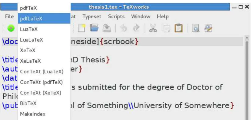
1.1 Selecting pdfLaTeX from the Drop-Down Menu. . . 3

1.2 Selecting BibTeX from the Drop-Down Menu . . . 4

1.3 Adding Makeglossaries to the list of tools in TeXworks . . . . 4

1.4 TeXwork’s Preferences Dialog Box . . . 6

1.5 Adding LaTeXmk in the TeXWorks Tool Configuration Dialog 6 1.6 LaTeXmk Tool Selected in TeXworks . . . 8

1.7 Arara Installer . . . 9

1.8 Adding Arara in the TeXWorks Tool Configuration Dialog . . 10

1.9 Using Arara in TeXworks . . . 11

4.1 Page Header and Footer Elements . . . 22

4.2 Sample Title Page . . . 26

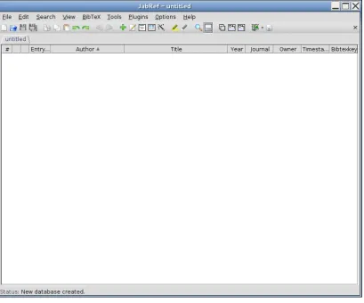
5.1 JabRef . . . 48

5.2 JabRef Preferences . . . 48

5.3 JabRef Database Properties . . . 49

5.4 JabRef (Select Entry Type) . . . 49

5.5 JabRef (New Entry) . . . 50

5.6 JabRef (Entering the Required Fields) . . . 51

5.7 JabRef (Entering Optional Fields) . . . 52

5.8 JabRef (Adding an Article) . . . 53

5.9 JabRef (Adding a Conference Paper) . . . 55

5.10 JabRef (Adding Editor List) . . . 56

5.11 Importing a Plain Text Reference . . . 57

5.12 Importing a Plain Text Reference (Selecting a Field) . . . 58

5.13 Importing a Plain Text Reference (Field Selected). . . 58

5.14 JabRef Advanced Preferences . . . 67

5.15 JabRef in BibLaTeX Mode . . . 67

5.16 JabRef in BibLaTeX Mode (Select Entry Type) . . . 68

5.17 JabRef in BibLaTeX Mode (Setting the Publication Date). . . . 69

(6)

List of Tables

4.1 Theorem Styles . . . 39

5.1 Name Formats for Bibliographic Data . . . 53

5.2 Standard BiBTeX entry types . . . 59

5.3 Standard BiBTeX fields . . . 60

5.4 Required and Optional Fields. . . 61

(7)

1 Getting Started . . . 14

2 Splitting a Large Document into Several Files (thesis.tex). 18 3 Splitting a Large Document into Several Files (intro.tex) . 19 4 Splitting a Large Document into Several Files (techintro.tex) 19 5 Splitting a Large Document into Several Files (method.tex). 19 6 Splitting a Large Document into Several Files (results.tex) 19 7 Splitting a Large Document into Several Files (conc.tex) . . 20

8 Changing the Page Style . . . 23

9 Double-Spacing . . . 24

10 Changing the Title Page . . . 24

11 Listings and Other Verbatim Text . . . 29

12 The amsthm Package . . . 35

13 The ntheorem Package. . . 40

14 Algorithms . . . 43

15 BibTeX. . . 63

16 Author–Year Citations . . . 65

17 Biblatex . . . 71

18 Creating an Index (makeidx package) . . . 74

19 Creating an Index (makeidx package) . . . 78

20 Creating Glossaries, Lists of Symbols or Acronyms (glossaries package) . . . 89

21 Using LA_{TEX to Sort and Collate Indexes or Glossaries (}_datagidx package) . . . 96

(8)

Abstract

This book is aimed at PhD students who want to use LA_{TEX to typeset their}

PhD thesis. If you are unfamiliar with LA_{TEX I recommend that you first}

read Volume 1: LA_{TEX for Complete Novices} [15].

(9)

Introduction

Many PhD students in the sciences are encouraged to produce their PhD thesis in LA_{TEX, particularly if their work involves a lot of mathematics. In}

addition, these days, LA_{TEX is no longer the sole province of mathematicians}

and computer scientists and is now starting to be used in the arts and so-cial sciences (see, for example, some of the topics listed in the TEX online catalogue [3]). This book is intended as a brief guide on how to typeset the various components that are usually required for a thesis. If you have never used LA_{TEX before, I recommend that you first read Volume 1:} _LA_TEX

for Complete Novices [15], as this book assumes you have a basic knowl-edge of LA_{TEX. As with Volume 1, I’ll be using PDFL}A_{TEX and TeXWorks. If}

you are creating a DVI file or you are using a different editor, you’ll have to

adapt the instructions.

B

If you are unfamiliar with terms such as “preamble”, read Volume 1[15, §2]. If you don’t know how to find package documentation, readVolume 1[15, §1.1].

Throughout this document there are pointers to related topics in theUK List of TEX Frequently Asked Questions1.1 _{(UK FAQ). These are displayed}

in the margin in square brackets, as illustrated on the right. You may find [FAQ: What is LaTeX?] these resources useful in answering related questions that are not covered

in this book.

On-line versions of this book, along with associated files, are available at: http://www.dickimaw-books.com/latex/thesis/. The links in this docu-ment are colour-coded: internal links are blue, external links are magenta.

To refresh your memory or for those who haven’t read Volume 1, through-out this book source code is illustrated in a typewriter font with the word Input placed in the margin, and the corresponding output (how it will appear in the PDF document) is typeset with the word Output in the margin.

Example:

A single line of code is displayed like this:

This is an \textbf{example}. Input

The corresponding output is illustrated like this:

This is an example. Output

Segments of code that are longer than one line are bounded above and below, illustrated as follows:

1.1_{http://www.tex.ac.uk/faq}

(10)

↑ Input

Line one\par

Line two\par

Line three.

↓ Input

with corresponding output:

↑ Output Line one

Line two Line three.

↓ Output

(Commands typeset in blue, such as \par, indicate a hyperlink to the com-mand definition in the summary.)

Command definitions are shown in a typewriter font in the form:

\documentclass[⟨options_⟩]{_⟨class őle_⟩} Definition

In this case the command being defined is called \documentclass and text

typed _⟨like this_⟩ (such as _⟨options_⟩ and _⟨class file_⟩) indicates the type of

thing you need to substitute. (Don’t type the angle brackets!) For example, if you want thescrbookclass file you would substitute_⟨class file_⟩withscrbook

and if you want theletterpaperoption you would substitute _⟨options_⟩with

letterpaper, like this:

\documentclass[letterpaper]{scrbook} Input When it’s important to indicate a space, the visible space symbol ␣ is used. For example:

A␣sentence␣consisting␣of␣six␣words. Input When you type up the code, replace any occurrences of ␣ with a space.

Note:

B

Be careful of the dangers of obsolete code propagation. It often happens that students pass on their LA_{TEX code to new students who, in their turn,}

pass it on to the next lot of students, and so on. You’re told “use this magic bit of code to format your thesis” without knowing what it does. Ancient buggy code that’s 20 years out-of-date festers in university departments refusing to die. But if it worked for previous students, what’s the problem? The problem is that it may stop working a week before your submission date and when you go for help, you may be told you’re using obsolete packages and there’s nothing for it but to rewrite your thesis using the modern alternatives.

How do you know if a package is obsolete? Some of the obsolete pack-ages and commands are listed in l2tabu [18], or you can check to see if a package is listed in _{the Comprehensive TEX Archive Network}1.2 _(CTAN)’s

obsolete tree (http://mirror.ctan.org/obsolete/). Stefan Kottwitz also has a list of obsolete classes and packages in his TeXblog. The other thing

(11)

to do is check the package’s entry on CTAN [2] to see if it has been depre-cated. For example, suppose someone tells you to use the glossary package. If you go to http://ctan.org/pkg/glossary it will tell you that the glossary package is no longer supported and that it’s been replaced by the glossaries package. Similarly, if you go tohttp://ctan.org/pkg/epsfigit will tell you that the epsfig package is obsolete and you should use graphicx instead.

1.1

Building Your Document

To “typeset”, “build”, “compile” or “LaTeX” your document means to run the

pdflatex (or latex) executable on your document source code. If you are

using a front-end, such as TeXworks, WinEdt, TeXstudio, or TeXnicCenter, this usually just means clicking on the appropriate button or selecting the appropriate menu item. (See Volume 1[15, §3] for further details.)

It’s important to remember that a front-end is an interface. It’s not, for example, TeXworks that is creating your PDF. When you click on the “typeset” button, TeXworks tells the operating system to run the required executable. This is usually pdflatex, but there are other executables that

may need to be used to help create your document, such as bibtex or biber (discussed in Chapter 5 (Generating a Bibliography)) and makeindex

or xindy (discussed inChapter 6 (Generating Indexes and Glossaries)).

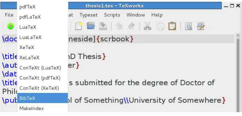
For example, if your document has a bibliography and you are using TeXworks, you first need to make sure the drop-down menu is set to “pdfLa-TeX” (seeFigure 1.1) and click on the green “Typeset” button. Then you need to select “BibTeX” from the drop-down menu (see Figure 1.2) and click on the green “Typeset” button. Then again select “pdfLaTeX” (Figure 1.1) and click the “Typeset” button. Finally, to ensure your cross-references are all up-to-date, you need to click on the “Typeset” button again. If you are using

biberinstead ofbibtex(seeSection 5.3), then you have to replace the above

“BibTeX” step with “Biber” instead.

(12)

Figure 1.2 Selecting BibTeX from the Drop-Down Menu

If the tool you require isn’t listed in the drop-down box, you will have to add it. For example, to add makeglossaries to the list of available tools

in TeXworks, you need to select EditÏPreferences, which will open the “TeX-works Preferences” dialog. Make sure the “Typesetting” tab is selected and click on the lower button next to the “Processing tools” list. This will open the “Tool Configuration” dialog. Set the “Name” field to the name of the application, as you want it to appear in the tool list (for example “MakeGlos-saries”). Then click on the “Browse” button to find the application on your computer. Next you need to click on the button next to the “Arguments” list. Set the argument to $basename. Since makeglossaries doesn’t modify

the PDF, uncheck the “View PDF after running” box (see Figure 1.3).

Figure 1.3 Adding Makeglossaries to the list of tools in TeXworks

(13)

even more so when you have glossaries and an index in your document as well as a bibliography. Fortunately there are ways of automating this process so that you only need one button press to perform all those dif-ferent steps. There are several applications available to do this for you, and I strongly recommend you try one of them, if possible, to reduce the complexity involved in building a document.

Volume 1 [15, §5.5] mentioned latexmk, which is available on CTAN [2].

This is a Perl script, so it will run on any operating system that has Perl installed (see Volume 1 [15, §2.20]). Since Volume 1 was published, a Java alternative called arara has arrived on CTAN [2]. Java applications will run

on any operating system that has the Java Runtime Environment installed, so both latexmk and arara are multi-platform solutions to automated

doc-ument compilation. Section 1.1.1 gives a brief introduction to latexmk, and

Section 1.1.2 gives a brief introduction to arara.

1.1.1

LaTeXmk

As mentioned above, latexmk is a Perl script that automates the process of

building a LA_{TEX document. In order to use} _latexmk_{, you must have Perl}

installed (see Volume 1 [15, §2.20]). Both TeX Live and MikTeX come with

latexmk but, if for some reason you don’t have it installed, you can use

the TeX Live or MikTeX update manager to install it. Alternatively, you can downloadhttp://mirror.ctan.org/support/latexmk.zip and install it manually.

Oncelatexmk is installed, you then need to add it to the list of available

tools in TeXworks1.3_{. This is done via the} _Edit_Ï_Preferences _{menu item. This}

opens TeXwork’s Preferences dialog box. Make sure the “Typesetting” tab is selected (Figure 1.4).

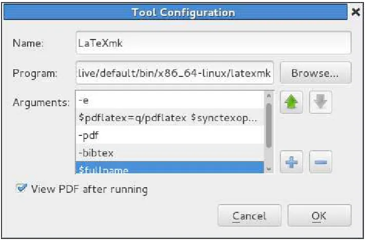
To add a new tool, click on the lower button next to the list of pro-cessing tools. This opens the tool configuration dialog box (Figure 1.5).

Type “LaTeXmk” in the “Name” box, then use the “Browse” button to locate latexmk on your computer. Next you need to click on the button

to add each argument. The argument list should consist of the following (in the order listed):

-e

$pdflatex=q/pdflatex $synctexoption %O %S/ -pdf

-bibtex $fullname

Once you’ve done this, click “Okay” to close the tool configuration dialog, and click “Okay” to close the Preferences dialog box. LaTeXmk should now be listed in the drop-down menu next to the green “Typeset” button. Now, if you have LaTeXmk selected and you click on the “Typeset” buttonpdflatex

and bibtex/biber will be run as necessary to create an up-to-date PDF.

(14)

Figure 1.4 TeXwork’s Preferences Dialog Box

(15)

Unfortunately, addingmakeindex,texindyormakeglossariesto LaTeXmk’s

set of rules is more complicated. For this you need to create a configura-tion/initialisation (RC) file1.4_{. The name and location of this file depends on}

your operating system. For example, on a Unix-like operating system, this may be $HOME/.latexmkrc. You will need to consult thelatexmk manual [1]

for further details.

Once you’ve found out the name and location of the RC file for your operating system, you can use the text editor of your choice to create this file. To add makeglossaries, you need to type the following in the RC file:

add_cus_dep(’glo’, ’gls’, 0, ’makeglossaries’); add_cus_dep(’acn’, ’acr’, 0, ’makeglossaries’); sub makeglossaries{

system( "makeglossaries \"$_[0]\"" ); }

To add makeindex, you need to type the following:

add_cus_dep(’idx’, ’ind’, 0, ’makeindex’); sub makeindex{

system("makeindex \"$_[0].idx\""); }

If you prefer to use texindy instead of makeindex, you will need to

re-place the above lines with (change the language as appropriate):

add_cus_dep(’idx’, ’ind’, 0, ’texindy’); sub texindy{

system("texindy -L english \"$_[0].idx\""); }

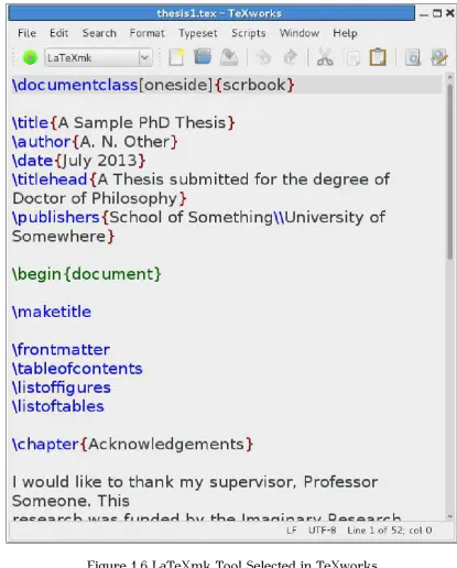
Now select “LaTeXmk” from the drop-down menu next to the green “Typeset” button in TeXworks (Figure 1.6), and you’re ready to build your documents.

1.1.2 Arara

As mentioned in Section 1.1, arara is a Java application that automates the

process of building a LA_{TEX document. In order to use}_arara_{, you must have}

the Java Runtime Environment installed. The latest TeX Live distribution includes arara, so you can install it via the TeX Live package manager.

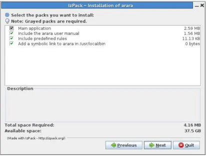
Alternative, you can installarara manually as follows: fetch the installer

arara-3.0-installer.jar (or arara-3.0-installer.exe) from https:// github.com/cereda/arara/tree/master/releases. On Windows, run

arara-3.0-installer.exe. On other operating systems run arara-3.0-installer.jar in privileged mode. For example, on a

Unix-based system:

(16)

(17)

Figure 1.7 Arara Installer

(If you are doing a manual install make sure you check the box to add the predefined rules, as shown in Figure 1.7.)

Oncearara has been installed, you can add it to the list of tools in

TeX-works. As before, open the TeXwork’s Preferences dialog box usingEditÏ Preferences and select the “Typesetting” tab (Figure 1.4).

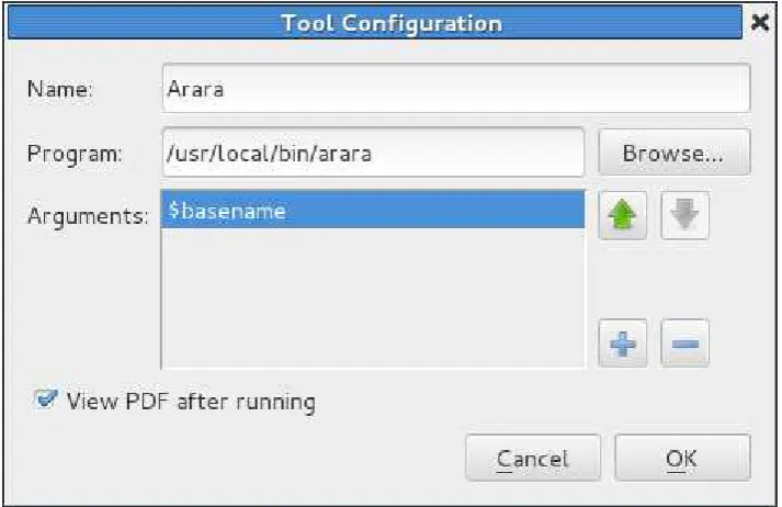
To add a new tool, click on the lower button next to the list of process-ing tools. This opens the tool configuration dialog box (Figure 1.8). Type “Arara” in the “Name” box and use the “Browse” button to find the arara

application on your computer. Use the button to add $basename to the

list of arguments, as shown in Figure 1.8.

Unlike latexmk, arara doesn’t read the log file to determine what

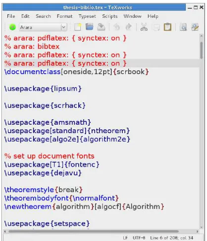
appli-cations need to be run. Instead, you tell arara how to build your document

by placing special comments in your source code. For example, if your document contains the following:

↑ Input % arara: pdflatex: { synctex: on }

% arara: bibtex

% arara: pdflatex: { synctex: on } % arara: pdflatex: { synctex: on } \documentclass{scrbook}

↓ Input

1.4_{There are some example RC files available at:} _{http://mirror.ctan.org/support/}

(18)

Figure 1.8 Adding Arara in the TeXWorks Tool Configuration Dialog

Then running arara on the document will run pdflatex, bibtex, pdflatex

and pdflatex on your document. Arara knows the rules “pdflatex” and

“bibtex”. It also knows the rules “biber”, “makeglossaries” and “makeindex”. So, if your document has a bibliography, an index and glossaries, you need to put the following comments in your source code (replace bibtex with biber if required):

% arara: bibtex

% arara: makeglossaries

% arara: makeindex

% arara: pdflatex: { synctex: on } % arara: pdflatex: { synctex: on } \documentclass{scrbook}

↓ Input

Now you just need to select “Arara” from the drop-down list in TeXworks (Figure 1.9) and click the green “Typeset” button, and arara will do all the

work for you.

Note:

B

If you don’t add these arara comments to your source code, nothing will happen when you run arara on your document! You must remember to

provide arara with the rules to build your document.

Unfortunately arara (v3.0) doesn’t have a rule for texindy, but you can

add one by creating a file called texindy.yamlthat contains the following:1.5

!config

# TeXindy rule for arara

(19)

(20)

# requires arara 3.0+ identifier: texindy name: TeXindy

command: <arara> texindy @{german} @{language} @{codepage} @{module}

Î˒

@{input} @{options} "@{getBasename(file)}.idx" arguments:

- identifier: german

flag: <arara> @{isTrue(parameters.german,"-g")} - identifier: language

flag: <arara> -L @{parameters.language} - identifier: codepage

flag: <arara> -C @{parameters.codepage} - identifier: module

flag: <arara> -M @{parameters.module} - identifier: input

flag: <arara> -I @{parameters.input} - identifier: options

flag: <arara> @{parameters.options}

(The symbolÎ˒ above indicates a line wrap. Don’t insert a line break at that point.) This file should be saved in the rules subdirectory of the arara

in-stallation directory. (For example, on Unix-like systems/usr/local/arara/ rules/texindy.yaml.)

So if you’d rather usetexindy instead of makeindexyou can replace the

% arara: makeindex

directive with

% arara: texindy: { language: english, codepage: latin1 }

(21)

Getting Started

There are many different thesis designs, varying according to university or discipline [5]. If you have been told to use a particular class file, use that one. If not, there are a selection of thesis class files available on CTAN [2] and listed in the _{OnLine TEX Catalogue’s Topic Index} [3]. Since there are so many to choose from, I’m just going to follow on from Volume 1 of this series and use one of the KOMA-Script class files. But which one? The scrreprt class is the one usually recommended for a report or thesis. It defaults to one-sided and has an abstract environment, but it doesn’t define

\frontmatter, \mainmatter or \backmatter. The scrbook class does define those commands, but it doesn’t provide anabstractenvironment and defaults

to two-sided layout. So, you can either do:

↑ Input \documentclass{scrreprt}

\title{A Sample Thesis} \author{A.N. Other}

\begin{document} \maketitle

\pagenumbering{roman} \tableofcontents

\chapter*{Acknowledgements}

\begin{abstract}

This is the abstract

\end{abstract}

\pagenumbering{arabic}

\chapter{Introduction}

...

\end{document}

↓ Input

or you can do:

(22)

↑ Input \documentclass[oneside]{scrbook}

\title{A Sample Thesis} \author{A.N. Other}

\frontmatter \tableofcontents

\chapter{Acknowledgements}

\chapter{Abstract}

This is the abstract

\mainmatter

\chapter{Introduction}

...

\end{document}

↓ Input

I’m going to use the second approach simply out of personal preference. The KOMA-Script options mentioned in this book are available for both scrreprt and scrbook, so choose whichever class file you feel best suits your thesis.

Unless you have been told otherwise, I recommend that you start out with a skeletal document that looks something like the following:

Listing 1

↑ Input

\documentclass[oneside]{scrbook}

\title{A Sample Thesis} \author{A.N. Other} \date{July 2013}

\titlehead{A Thesis submitted for the degree of Doctor of Philosophy} \publishers{School of Something\\University of Somewhere}

(23)

I would like to thank my supervisor, Professor Someone. This research was funded by the Imaginary Research Council.

\chapter{Abstract}

A brief summary of the project goes here.

% A glossary and list of acronyms may go here

% or may go in the back matter.

\mainmatter

\chapter{Introduction} \label{ch:intro}

\chapter{Technical Introduction} \label{ch:techintro}

\chapter{Method} \label{ch:method}

\chapter{Results} \label{ch:results}

\chapter{Conclusions} \label{ch:conc}

\backmatter

% A glossary and list of acronyms may go here

% or may go in the front matter after the abstract.

% The bibliography will go here

\end{document}

↓ Input

If you do this, it will help ensure that your document has the correct structure before you begin with the actual contents of the document. (Note that the chapter titles will naturally vary depending on your subject or in-stitution, and you may need a different paper size if you are not in Europe. I have based the above on my own PhD thesis which I wrote in the early to mid 1990s in the Department of Electronic Systems Engineering at the University of Essex, and it may well not fit your own requirements.)

(24)

which can give you a sense of achievement that can help give you sufficient momentum to get started (but of course, it’s not guaranteed to work with everyone). Remember that if you want to use arara (see Section 1.1.2) you

must add the build rules to the document:

% arara: pdflatex: { synctex: on } \documentclass[oneside]{scrbook}

↓ Input

(I’ll add the arara rules to sample listings, in the event that you want to use arara. Since they are comments, they will be ignored if you use pdflatex

explicitly or if you use another automation method, such as latexmk.)

Now think about other requirements. What font size have you been told to use?

10pt Use the 10ptclass option:

\documentclass[oneside,10pt]{scrbook} Input

11pt Use the11pt class option:

12pt Use the 12pt class option:

Have you been told to have a blank line between paragraphs and no para-graph indentation? If so, use the parskip=full class option:

\documentclass[oneside,12pt,parskip=full]{scrbook} Input

Have you been told to have certain sized margins? If so, you can use the [FAQ: Changing the margins in LA_TEX_]

geometry package. For example, if you have been told you must have 1 inch margins, you can do

(25)

Splitting a Large Document

into Several Files

Some people prefer to place each chapter of a large document in a separate file and then input the file into the main document.

There are two basic ways of including the contents of an external file:

\input{_⟨őlename_⟩} Definition

and

\include{_⟨őlename_⟩} Definition

where _⟨őlename_⟩ is the name of the file. (The .tex extension may be

omitted in both cases.) The differences between the two commands are as follows:

\input acts as though the contents of the file were typed where the\input command was. For example, suppose my main file contained the fol-lowing:

↑ Input

Here is a short paragraph.

\input{myfile}

↓ Input

and suppose the file myfile.tex contained the following lines:

↑ Input

Here is some sample text.

↓ Input

then the \input command behaves as though you had simply typed the following in your main document file:

↑ Input

(26)

Here is a short paragraph.

Here is some sample text.

↓ Input

\include does more than just input the contents of the file. It also starts a new page (using \clearpage) and creates an auxiliary file associated with the included file. It also issues another \clearpage once the file has been read in. Using this approach, you can also govern which files to include using

\includeonly{_⟨őle list_⟩} Definition

in the preamble, where _⟨őle list_⟩ is a comma-separated list of files you want included. This way, if you only want to work on one or two chapters, you can only include those chapters, which will speed up the document build. LA_{TEX will still read in all the cross-referencing}

information for the missing chapters, but won’t include those chapters in the PDF file. There is a definite advantage to this if you have, say, a large number of images in your results chapter, which you don’t need when you’re working on, say, the technical introduction. You can still reference all the figures in the omitted chapter, as long as you have previouslyLA_{TEXed the document}_{without the} _\includeonly_command. The excludeonly package provides the logically opposite command:

\excludeonly{_⟨őle list_⟩} Definition

The previous example can now be split into various files:

Listing 2 (thesis.tex)

↑ Input

% arara: pdflatex: { synctex: on } % arara: pdflatex: { synctex: on } \documentclass[oneside]{scrbook}

\title{A Sample Thesis} \author{A.N. Other} \date{July 2013}

\titlehead{A Thesis submitted for the degree of Doctor of Philosophy} \publishers{School of Something\\University of Somewhere}

(27)

\listoftables

I would like to thank my supervisor, Professor Someone. This research was funded by the Imaginary Research Council.

\chapter{Abstract}

A brief summary of the project goes here.

\mainmatter

\include{intro}

\include{techintro}

\include{method}

\include{results}

\include{conc}

\backmatter

\end{document}

↓ Input

Listing 3 (intro.tex)

↑ Input \chapter{Introduction}

\label{ch:intro}

↓ Input

Listing 4 (techintro.tex)

↑ Input \chapter{Technical Introduction}

\label{ch:techintro}

↓ Input

Listing 5 (method.tex)

↑ Input \chapter{Method}

\label{ch:method}

↓ Input

Listing 6 (results.tex)

↑ Input \chapter{Results}

\label{ch:results}

(28)

Listing 7 (conc.tex)

↑ Input \chapter{Conclusions}

\label{ch:conc}

↓ Input

If you only want to work on, say, the Method and Results chapters, you can place the following command in the preamble:

(29)

Formatting

It used to be that in order to change the format of chapter and section headings, you needed to have some understanding of the internal workings of classes such as report or book. Modern classes, such as memoir and the KOMA-Script classes, provide a much easier interface. However, I recom-mend that you first write your thesis, and then worry about changing the document style. The ability to separate content from style is one of the ad-vantages of using LA_{TEX over a word processor. Remember that writing your}

thesis is more important than the layout. Whilst it may be that your school or department insists on a certain style, it should not take precedence over the actual task of writing.

4.1 Changing the Document Style

If you are using a custom thesis class file provided by your department or school, then you should stick to the styles set up in that class. If not, you may need to change the default style of your chosen class to fit the requirements.

Volume 1 [15, §5.3] described how to change the fonts used by chapter and section headings for the KOMA-Script classes. For example, if the chapter headings must be set in a large, bold, serif font you can do:

\addtokomafont{\large\bfseries\rmfamily} Input

The headings in the KOMA-Script classes default to ragged-right justification (recall \raggedright from §2.12 of Volume 1) which is done via

\raggedsection Definition

This can be redefined as required. For example, suppose you are required to have centred headings, then you can do:

\renewcommand*{\raggedsection}{\centering} Input

4.2 Changing the Page Style

Volume 1 [15, §5.7] described the command

\pagestyle{_⟨style_⟩} Definition

which can be used to set the page style. The scrbook class defaults to the

headings page style, but if this isn’t appropriate, you can use the scrpage2

(30)

package, which comes with the KOMA-Script bundle. This package pro-vides its own versions of theplainandheadingspage styles, calledscrplain

and scrheadings.

For simplicity, I’m assuming that your thesis is a one-sided document. If this isn’t the case and your odd and even page styles need to be different, you’ll need to consult the KOMA-Script documentation [8].

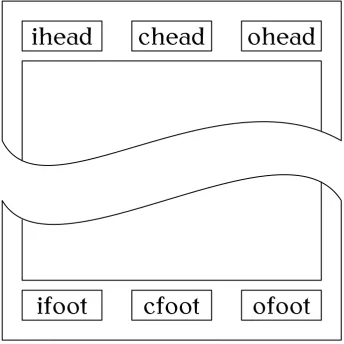
With the scrheadings page style, the page header and footer are both

divided into three areas (Figure 4.1): the inner (left) head/foot, the centre head/foot and the outer (right) head/foot.

ihead

chead

ohead

ifoot

cfoot

ofoot

Figure 4.1 Page Header and Footer Elements

These elements can be set using:

\ihead[_⟨scrplain inner head_⟩]{_⟨scrheadings inner head_⟩} \chead[_⟨scrplain centre head_⟩]{_⟨scrheadings centre head_⟩} \ohead[_⟨scrplain outer head_⟩]{_⟨scrheadings outer head_⟩} \ifoot[_⟨scrplain inner foot_⟩]{_⟨scrheadings inner foot_⟩} \cfoot[_⟨scrplain centre foot_⟩]{_⟨scrheadings centre foot_⟩} \ofoot[_⟨scrplain outer foot_⟩]{_⟨scrheadings outer foot_⟩}

Definition

In each case, the optional argument indicates what to do if the scrplain

page style is in use and the mandatory argument indicates what to do if the

(31)

modification is made to thescrplainstyle.) Within both types of argument,

you can use

\pagemark Definition

to insert the current page number and

\headmark Definition

to insert the running heading. For example, suppose you are required to put your registration number on the bottom left of each page and the page number on the bottom right, and you are also required to put the current chapter or section heading at the top left of each page, unless it’s the first page of a chapter. Then you can do:

Listing 8

↑ Input \usepackage{scrpage2}

\pagestyle{scrheadings}

\newcommand{\myregnum}{123456789}% registration number

\ihead{} \chead{}

\ohead[]{\headmark}

\ifoot[\myregnum]{\myregnum}% registration number

\cfoot[]{}

\ofoot[\pagemark]{\pagemark}

↓ Input

Note that the above don’t use any font changing commands. If you want to change the font for the header and footer, you need to redefine \headfont. The page number style is given by \pnumfont. So for italic headers and footers with bold page numbers, you can redefine these com-mands as follows:

↑ Input \renewcommand*{\headfont}{\normalfont\itshape}

\renewcommand*{\pnumfont}{\normalfont\bfseries}

↓ Input

4.3 Double-Spacing

Whilst double-spacing is usually frowned upon in the world of modern type-setting, it is usually a requirement for anything that may need hand-written annotations, which can include theses. This extra space gives the examiners room to write comments.4.1

4.1_{Despite the current digital age, many people still use hand-written annotations on}

(32)

Double-spacing can be achieved via thesetspacepackage. You can either set the spacing using the package options singlespacing, onehalfspacing

or doublespacing, or you can switch via the declarations:

\singlespacing \onehalfspacing \doublespacing

Definition

So, if your thesis has to be double-spaced, you can do:

Listing 9

↑ Input \usepackage[doublespacing]{setspace}

↓ Input

4.4

Changing the Title Page

Volume 1[15, §5.1] described how to lay out the title page using\maketitle. If this layout isn’t appropriate for your school or department’s specifications, you can lay out the title page manually using thetitlepageenvironment instead

of\maketitle. Within this environment, you can use\hspace{_⟨length_⟩}and \vspace{_⟨length_⟩} to insert horizontal and vertical spacing. (The unstarred versions are ignored if they occur at the start of a line or page, respectively. The starred versions will insert the given spacing, regardless of their lo-cation.) You can also use \hfill and \vfill, which will expand to fill the available space horizontally or vertically, respectively.

Example:

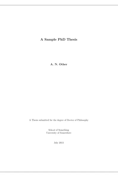
Listing 10

↑ Input \begin{titlepage}

\centering \vspace*{1in}

\begin{Large}\bfseries

A Sample PhD Thesis\par \end{Large}

\vspace{1.5in}

\begin{large}\bfseries

A. N. Other\par \end{large} \vfill

A Thesis submitted for the degree of Doctor of Philosophy

\par

\vspace{0.5in}

School of Something

\par

University of Somewhere

\par

(33)

July 2013

\par

\end{titlepage}

↓ Input

The result is shown in Figure 4.2. (If you require double-spacing, you may need to wait until after the title page before switching to double-spacing.)

4.5

Listings and Other Verbatim Text

[FAQ: Code listings in LA_TEX_] There may be times when you want to include text exactly as you have

typed it into your source code. For example, you may want to include a short segment of computer code. This can be done using the verbatim

environment.

Example:

Note how I don’t need to worry about special characters, such as #, within

the verbatim environment:

↑ Input \begin{verbatim}

#include <stdio.h> /* needed for printf */

int main() {

printf("Hello World\n");

return 1; }

\end{verbatim}

↓ Input

This just produces:

↑ Output

int main() {

return 1; }

↓ Output

A more sophisticated approach is to use the listings package. With this package, you first need to specify the programming language. For example, the above code is in C, so I need to specify this using:

\lstset{language=C} Input

(34)

A Sample PhD Thesis

A. N. Other

A Thesis submitted for the degree of Doctor of Philosophy

School of Something University of Somewhere

July 2013

(35)

↑ Input \begin{lstlisting}

int main() {

return 1; }

\end{lstlisting}

↓ Input

The resulting output looks like:

↑ Output #include <s t d i o . h> / ∗ needed f o r p r i n t f ∗ /

i n t main ( ) {

p r i n t f ( " Hello World\n " ) ;

return 1 ;

}

↓ Output

I can also have inline code snippets using:

\lstinline[_⟨options_⟩]_⟨char_⟩⟨code_⟩⟨char_⟩ Definition

This is different syntax to the usual forms of command argument. You can chose any character _⟨char_⟩ that isn’t the open square bracket [ and that doesn’t occur in _⟨code_⟩ to delimit the code, but the start and end _⟨char_⟩ must match. (The optional argument is discussed below.) So the following are all equivalent:

1. _⟨char_⟩ is the exclamation mark character:

\lstinline!#include <stdio.h>! Input

2. _⟨char_⟩ is the vertical bar character:

\lstinline|#include <stdio.h>| Input

3. _⟨char_⟩ is the double-quote character:

\lstinline"#include <stdio.h>" Input

4. ⟨char_⟩ is the plus symbol:

\lstinline+#include <stdio.h>+ Input

(36)

↑ Input

The stdio header file (required for the \lstinline+printf+ function) is loaded using the directive \lstinline!#include <stdio.h>! on the first line.

↓ Input

Result:

↑ Output The stdio header file (required for the printf function) is loaded using

the directive #include <stdio.h> on the first line.

↓ Output

Another alternative is to input the code from an external file. For ex-ample, suppose my C code is contained in the filehelloworld.c, then I can

input it using:

\lstinputlisting[_⟨options_⟩]{helloworld.c} Input (Remember to use a forward slash / as the directory divider, even if you

are using Windows.)

All the above (\lstinline, \lstinputlisting and the lstlisting

environ-ment) have an optional argument _⟨options_⟩ that can be used to override the default settings. These are ⟨key_⟩=⟨value_⟩ options. There are a lot of options available, but I’m only going to cover a few. If you want more detail, have a look at the listings documentation [6].

title={_⟨text_⟩} is used to set an unnumbered and unlabelled title. If _⟨text_⟩ contains a comma or equal sign, make sure you enclose⟨text_⟩in curly braces { and }.

caption={[_⟨short_⟩]_⟨text_⟩} is used to set a numbered caption. The optional part_⟨short_⟩is an alternative short caption for the list of listings, which can be produced using

\lstlistoflistings Definition

As above, if the caption contains a comma or equal sign, make sure you enclose it in curly braces { and }.

label={_⟨text_⟩} is used to assign a label to this listing so the number can be referenced via \ref.

numbers={_⟨setting_⟩} The value_⟨setting_⟩may be one of: none(no line

num-bers), left (line numbers on the left) or right (line numbers on the

right).

mathescape This is a boolean key that can either be true (dollar $ charac-ter acts as the usual math mode shift) or false (deactivates the usual

behaviour of $).

basicstyle={_⟨declaration_⟩} The value (one or more declarations) is used at the start of the listing to set the basic font style. For example,

(37)

Note:

B

If you setbasicstyleto\ttfamilyand you want bold keywords, make sure you are using a typewriter font that supports bold, as not all of them do. (Recall fromVolume 1[15, §4.5.3] how to change the font family.) This book uses txtt (see Volume 1[15, §8.2]). Other possibilities include beramono, tgcur-sor, courier, DejaVuSansMono (or dejavu to load the serif and sans-serif DejaVu fonts as well), lmodern and luximono.

KOMA and listings

B

If you want to use the listingspackage with one of the KOMA-Script classes, you need to load scrhack before listings, otherwise you will get a warning that looks like:

Class scrbook Warning: Usage of deprecated \float@listhead!

(scrbook) You should use the features of package ‘tocbasic’ (scrbook) instead of \float@listhead.

(scrbook) Definition of \float@listhead my be removed from (scrbook) ‘scrbook’ soon, so it should not be used on input line 57.

Example:

Listing 11

↑ Input

\begin{lstlisting}[language=C,basicstyle=\ttfamily, mathescape=true]

#include <stdio.h> /* needed for printf */ #include <math.h> /* needed for sqrt */

int main() {

double x = sqrt(2.0); /* $x = \sqrt{2}$ */

printf("x = %f\n", x);

return 1; }

\end{lstlisting}

↓ Input

Result:

↑ Output

# include < stdio .h > /* needed for printf */

# include <math .h > /* needed for sqrt */

int main () {

(38)

printf ("x␣=␣%f\n" , x );

return 1; }

↓ Output

If you are using double-spacing, you may need to temporarily switch it off in the listings. You can do this by adding \singlespacingto thebasicstyle

setting.

\lstset{basicstyle={\ttfamily\singlespacing}} Input (Check with your supervisor to find out if listings should be double- or single-spaced.)

Note:

It is not usually appropriate to have reams of listings in your thesis. It can annoy an examiner if you have included every single piece of code you have written during your PhD, as it comes across as padding to make it look as though your thesis is a lot larger than it really is. (Examiners are not easily fooled, and it’s best not to irritate them as it is likely to make them less sympathetic towards you.) If you want to include listings in your thesis, check with your supervisor first to find out whether or not it is appropriate.

B

Be careful when you use verbatim-like environments or commands, such

asverbatim,lstlisting,\lstinlineand\lstinputlisting. In general, they can’t

be used in the argument of another command. [FAQ: Why

doesn’t verbatim work within . . . ?]

4.6 T

abbing

The tabbing environment lets you create tab stops so that you can tab to

a particular distance from the left margin. Within the tabbing environment, you can use the command \= to set a tab stop, \> to jump to the next tab stop, \< to go back a tab stop, \+ to shift the left border by one tab stop to the right, \- to shift the left border by one tab stop to the left. In addition, \\ will start a new line and\kill will set any tabs stops defined in that line, but will not typeset the line itself.

Note:

B

You may recall two of the above commands from Volume 1: \- was de-scribed as a discretionary hyphen in §2.14 and \= was described as the macron accent command in §4.3. These two commands take on

differ-ent meanings when they are used in the tabbing environment. If you want [FAQ: Accents misbehave in

tabbing] accents in your tabbing environment, either use the inputenc package (see

Volume 1 [15, §4.3.1]) or use \a_⟨accent symbol_⟩{_⟨c_⟩}, for example \a"{u}

(39)

Example:

↑ Input \begin{tabbing}

Zero \=One \=Two \=Three\\ \>First tab stop\\

\>A\>\>B\\

\>\>Second tab stop

\end{tabbing}

↓ Input

This produces the following output:

↑ Output

Zero One Two Three First tab stop

A B

Second tab stop

↓ Output

Another Example:

This example sets up four tab stops, but ignores the first line:

↑ Input \begin{tabbing}

AAA \=BBBB \=XX \=YYYYYY \=Z \kill \>\>\>Third tab stop\\

\>a \>b \> \>c

\end{tabbing}

↓ Input

This produces the following output:

↑ Output

Third tab stop

a b c

(40)

4.7

Theorems

A PhD thesis can often contain theorems, lemmas, definitions etc. The LA_TEX

kernel comes with the command:

\newtheorem{_⟨name_⟩}[_⟨counter_⟩]{_⟨title_⟩}[_⟨outer counter_⟩] Definition

which can be used to create an environment called _⟨name_⟩ that has an optional argument. Each instance of the environment starts with ⟨title_⟩ followed by the associated counter value. If _⟨counter_⟩ is present, the new environment uses that counter instead of having a new counter defined for it. If ⟨outer counter_⟩ is present, the environment counter is reset every time _⟨outer counter_⟩ is incremented. The optional arguments are mutually exclusive.

In the example below, I’ve use\newtheoremto define a new environment called theorem, which has an associated counter, also called theorem, that is dependant on the chapter counter.

↑ Input % in the preamble:

\newtheorem{theorem}{Theorem}[chapter]

% later in the document:

\begin{theorem}

If proposition $P$ is a tautology then $\sim P$ is a contradiction, and conversely.

\end{theorem}

↓ Input

Resulting output:

↑ Output

Theorem 4.1 If proposition 𝑃 is a tautology then _∼𝑃 is a contradiction, and conversely.

↓ Output

The optional argument to the new environment can be used to add a caption. Modifying the above example (changes shown like this):

\newtheorem{theorem}{Theorem}[chapter]

\begin{theorem}[Tautologies and Contradictions]

\end{theorem}

(41)

Resulting output:

↑ Output

Theorem 4.2 (Tautologies and Contradictions) If proposition 𝑃 is a ta

u-tology then ∼ 𝑃 is a contradiction, and conversely.

↓ Output

Here’s an example that uses the first optional argument of \newtheorem:

\newtheorem{exercise}{Exercise}

\newtheorem{suppexercise}[exercise]{Supplementary Exercise}

\begin{exercise}

This is an example of how to create a theorem-like environment.

\end{exercise}

\begin{suppexercise}

This is another example of how to create a theorem-like environment.

\end{suppexercise}

↓ Input

Result:

↑ Output

Exercise 1 This is an example of how to create a theorem-like environ-ment.

Supplementary Exercise 2 This is another example of how to create a theorem-like environment.

↓ Output

Unfortunately there isn’t a great deal of flexibility with the environment

appearance. However there are various packages available that provide en- [FAQ: Theorem bodies printed in a roman font] hancements to this basic command, allowing you to adjust the appearance

to suit your requirements. There seem to be two main contenders: amsthm and ntheorem. Both have advantages and disadvantages. For example, nthe-orem is more flexible but amsthm is more robust. Therefore I’m going to describe both, and you will have to decide which one you prefer.

Note:

B

If you are using either packages with amsmath, you must load amsmath first:

↑ Input \usepackage{amsmath}

\usepackage{ntheorem}

↓ Input

(42)

↑ Input \usepackage{amsmath}

\usepackage{amsthm}

↓ Input

With bothamsthm and ntheorem, you can still define new theorem-like en-vironments using \newtheorem, but there is also a starred version of that command, which can be used to define unnumbered theorem-like environ-ments.

Example:

Suppose I want to have an unnumbered remark environment, I can define the environment like this:

\newtheorem*{note}{Note}

\begin{note}

This is a note about something.

\end{note}

↓ Input

Result:

↑ Output Note This is a note about something.

↓ Output

4.7.1 The

amsthm

Package

Theamsthmpackage provides three predefined theorem styles: plain,definition

andremark. When you define a new theorem-like environment with\newtheorem, it is given the style currently in effect. You can change the current style with:

\theoremstyle{_⟨style name_⟩} Definition

where _⟨style name_⟩ is the name of the theorem style.

Example:

(43)

↑ Input \theoremstyle{plain}

\newtheorem{theorem}{Theorem} \newtheorem{lemma}{Lemma}

\theoremstyle{definition} \newtheorem{defn}{Definition} \newtheorem{conj}{Conjecture}

\theoremstyle{remark} \newtheorem*{note}{Note} \newtheorem{remark}{Remark}

↓ Input

The amsthm package also provides the proof environment, which can be

used for typesetting proofs.

\begin{proof}[_⟨title_⟩] Definition

The optional argument _⟨title_⟩ is a replacement for the default title. This environment automatically inserts a QED symbol at the end of it, but if the default location isn’t appropriate (which can happen if the proof ends with an equation) then use

\qedhere Definition

where you want the QED symbol to appear. The symbol is given by

\qedsymbol Definition

This defaults to an unfilled square , but you can redefine \qedsymbol to something else if you prefer. (Recall redefining commands from Vol-ume 1 [15, §8.2].)

Listing 12

↑ Input

% in the preamble:

\usepackage{amsthm} \theoremstyle{plain}

\newtheorem{theorem}{Theorem}

\theoremstyle{definition} \newtheorem{defn}{Definition}

\newtheorem{xmpl}{Example}[chapter]

\theoremstyle{remark}

\newtheorem{remark}{Remark}

(44)

\begin{defn}[Tautology]\label{def:tautology}

A \emph{tautology} is a proposition that is always true for any value of its variables.

\end{defn}

\begin{defn}[Contradiction]\label{def:contradiction}

A \emph{contradiction} is a proposition that is always false for any value of its variables.

\end{defn}

\begin{theorem}

\begin{proof}

If $P$ is a tautology, then all elements of its truth table are true (by Definition~\ref{def:tautology}), so all elements of the truth table for $\sim P$ are false, therefore $\sim P$ is a contradiction (by Definition~\ref{def:contradiction}).

\end{proof} \end{theorem}

\begin{xmpl}\label{ex:rain}

‘‘It is raining or it is not raining’’ is a tautology, but ‘‘it is not raining and it is raining’’ is a contradiction.

\end{xmpl}

\begin{remark}

Example~\ref{ex:rain} used De Morgan’s Law $\sim (p \vee q)

\equiv \sim p \wedge \sim q$.

\end{remark}

↓ Input

Result:

↑ Output Definition 1 (Tautology). A tautology is a proposition that is always true

for any of its variables.

Definition 2(Contradiction). A contradictionis a proposition that is always false for any value of its variables.

Theorem 4.3. If proposition 𝑃 is a tautology then ∼ 𝑃 is a contradiction, and conversely.

𝑃roof. If 𝑃 is a tautology, then all elements of its true table are true (by Definition 1), so all elements of the truth table for ∼ 𝑃 are false, therefore ∼ 𝑃 is a contradiction (by Definition 2).

Example 1. “It is raining or it is not raining” is a tautology, but “it is not

(45)

Remark 1. Example 1 used De Morgan’s Law ∼(𝑝∨𝑞)≡∼𝑝∧ ∼𝑞.

↓ Output

A new theorem style can be created using

\newtheoremstyle{_⟨name_⟩}{_⟨space above_⟩}{_⟨space below_⟩}{_⟨body font_⟩}{_⟨indent_⟩}{_⟨head font_⟩}{_⟨post head punctuation_⟩}{_⟨post head space_⟩}{_⟨head spec_⟩}

Definition

This defines a new theorem style called_⟨name_⟩, which can later be set using \theoremstyle. The other arguments are as follows:

⟨space above_⟩ the amount of space above the theorem-like en-vironment

⟨space below_⟩ the amount of space below the theorem-like en-vironment

⟨body font_⟩ the font to be used in the main theorem body

⟨indent_⟩ the amount of indentation (empty means no in-dent or use \parindentfor normal paragraph in-dentation)

⟨head font_⟩ the font to be used in the theorem header

⟨post head punctuation_⟩ the punctuation to be inserted after the theorem head

⟨post head space_⟩ the space to put after the theorem head (use {␣} for a normal interword space or \newline for a linebreak)

⟨head spec_⟩ the theorem head spec

Example:

This example creates a new style called note that inserts a space of 2ex

above the theorem and 2ex below.4.2 _{The body font is just the normal font.}

There is no indent, the theorem header is in small caps, a full stop is put after the theorem head and a line break is inserted between the theorem head and body:

↑ Input \newtheoremstyle{note}% style name

{2ex}% above space

{2ex}% below space

{}% body font

{}% indent amount

{\scshape}% head font

{.}% post head punctuation

{\newline}% post head punctuation

(46)

↓ Input

Once you have defined the style, you can now use it. For example (in the preamble):

↑ Input \theoremstyle{note}

\newtheorem{scnote}{Note}

↓ Input

This defines a theorem-like environment called scnote. You can now use it later in the document:

↑ Input \begin{scnote}

This is an example of a theorem-like environment.

\end{scnote}

↓ Input

This produces:

↑ Output N_{ote 1.}

This is an example of a theorem-like environment.

↓ Output

4.7.2

The

ntheorem

Package

The ntheorempackage provides nine predefined theorem styles, listed in Ta-ble 4.1. The default is plain. When you define a new theorem-like

envi-ronment with\newtheorem, it is given the style currently in effect. You can change the current style with:

\theoremstyle{_⟨style name_⟩} Definition

where _⟨style name_⟩ is the name of the theorem style. In addition to these styles, you can also use

\theoremheaderfont{_⟨declarations_⟩} Definition

to set the header font to _⟨declarations_⟩, which should consist of font decla-ration commands such as \normalfont,

\theorembodyfont{_⟨declarations_⟩} Definition

to set the body font to ⟨declarations_⟩, and

\theoremnumbering{_⟨style_⟩} Definition

(47)

Table 4.1 Predefined Theorem Styles Provided by ntheorem

plain Like the original LA_{TEX style}

break Header is followed by a line break

change Like plain but header and number interchanged changebreak Combination of change and break

margin Number is set in the margin

marginbreak Like margin but header followed by a line break nonumberplain Like plain but without the number

nonumberbreak Like break but without the number

empty No number and no name. Only the optional

argu-ment is used in the header.

to set the appearance of the theorem number, where _⟨style_⟩ may be one of: arabic, roman, Roman, alph, Alph,greek, Greek or fnsymbol. Remember

that the above commands all need to be used before the new theorem-like environment is defined. For additional commands that affect the style of the theorems, see the ntheorem documentation [10].

Example:

\theoremstyle{marginbreak} \theorembodyfont{\normalfont} \newtheorem{note}{Note}[chapter]

\begin{note}

This is a sample note. The number is in the margin.

\end{note}

↓ Input

Result:

↑ Output

4.1 Note

This is a sample note. The number is in the margin.

↓ Output

If you use the standard package option to ntheorem, it will automatically define the following environments: Theorem, Lemma, Proposition, Corollary, Satz, Korollar, Definition, Example, Beispiel, Anmerkung, Bemerkung, Remark, Proof and

Be-weis.

B

Unlike amsthm’s proof environment, ntheorem’s Proof environment appends its optional argument in parentheses, if present, to the proof title. (Recall from earlier thatamsthm’sproof environment uses its optional argument as a

(48)

Example:

Listing 13

↑ Input

% in the preamble:

\usepackage[standard]{ntheorem}

\begin{Definition}[Tautology]\label{def:tautology}

A \emph{tautology} is a proposition that is always true for any value of its variables.

\end{Definition}

\begin{Definition}[Contradiction]\label{def:contradiction}

A \emph{contradiction} is a proposition that is always false for any value of its variables.

\end{Definition}

\begin{Theorem}

\begin{Proof}

If $P$ is a tautology, then all elements of its truth table are true (by Definition~\ref{def:tautology}), so all elements of the truth table for $\sim P$ are false, therefore $\sim P$ is a contradiction (by Definition~\ref{def:contradiction}).

\end{Proof} \end{Theorem}

\begin{Example}\label{ex:rain}

‘‘It is raining or it is not raining’’ is a tautology, but ‘‘it is not raining and it is raining’’ is a contradiction.

\end{Example}

\begin{Remark}

Example~\ref{ex:rain} used De Morgan’s Law $\sim (p \vee q)

\equiv \sim p \wedge \sim q$.

\end{Remark}

↓ Input

Result:

↑ Output Definition 3 (Tautology) A tautology is a proposition that is always true

for any value of its variables.

(49)

Theorem 4.4 If proposition 𝑃 is a tautology then ∼ 𝑃 is a contradiction, and conversely.

Proof _If 𝑃 _{is a} tautology, then all elements of its truth table are true (by Definition 3), so all elements of the truth table for ∼ 𝑃 are false, therefore ∼ 𝑃 is a contradiction (by Definition 4).

Example 2 “It is raining or it is not raining” is a tautology, but “it is not

raining and it is raining” is a contradiction.

Remark 2 Example 2 used De Morgan’s Law∼₍𝑝∨𝑞)≡∼𝑝∧ ∼𝑞.

↓ Output

4.8 Algorithms

If you want to display an algorithm, such as pseudo-code, you can use a com-bination of thetabbingenvironment (described inSection 4.6) and a

theorem-like environment (described above in Section 4.7).

Example:

\theoremstyle{break}

\theorembodyfont{\normalfont} \newtheorem{algorithm}{Algorithm}

\begin{algorithm}[Gauss-Seidel Algorithm] \begin{tabbing}

1. \=For $k=1$ to maximum number of iterations\\ \>2. For \=$i=1$ to $n$\\

\>\>Set

\begin{math}

x_i^{(k)} =

\frac{b_i-\sum_{j=1}^{i-1}a_{ij}x_j^{(k)}

-\sum_{j=i+1}^{n}a_{ij}x_j^{(k-1)}}% {a_{ii}}

\end{math} \\

\>3. If $\lvert\vec{x}^{(k)}-\vec{x}^{(k-1)}\rvert < \epsilon$, where $\epsilon$ is a specified stopping criteria, stop.

\end{tabbing} \end{algorithm}

↓ Input

(50)

↑ Output

Algorithm 1 (Gauss-Seidel Algorithm)

1. For_𝑘 =1 to maximum number of iterations 2. For 𝑖 = 1 to 𝑛

Set 𝑥_𝑖(𝑘) = 𝑏𝑖−∑︀𝑖−𝑗=11𝑎𝑖𝑗𝑥(𝑗𝑘)− ∑︀𝑛

𝑗=𝑖+1𝑎𝑖𝑗𝑥𝑗(𝑘−1)

𝑎𝑖𝑖

3. If ♣𝑥⃗(𝑘)₋_𝑥_⃗(𝑘−1)_♣_{< 𝜖}_{, where} _𝜖 _{is a specified stopping criteria, stop.}

↓ Output

(See Volume 1 [15, §9.4.11] to find out how to redefine \vec to display its argument in bold.)

If you want a more sophisticated approach, there are some packages available on CTAN [2], such as alg, algorithm2e, algorithms and algorithmicx. I’m going to briefly introduce thealgorithm2epackage here. This provides the

al-gorithmfloating environment. Like thefigureandtableenvironments described

inVolume 1[15, §7], thealgorithmenvironment has an optional argument that

specifies the placement.

\begin{algorithm}[_⟨placement_⟩] Definition

If you are using a class or package that already defines analgorithm environ-ment, you can use the algo2e package option:

\usepackage[algo2e]{algorithm2e} Input This will define an environment calledalgorithm2einstead ofalgorithmto avoid

conflict.

Within the body of the environment, you must mark the end of each line with \; regardless of whether you want a semi-colon to appear. To suppress the default end-of-line semi-colon, use

\DontPrintSemicolon Definition

To switch it back on again, use

\PrintSemicolon Definition

There are a variety of commands that may be used within thealgorithm

envi-ronment. Some of the commands are described below, but for a complete list you should consult the algorithm2e documentation [4].

First there are the commands for the algorithm input, output and data:

\KwIn{_⟨input_⟩} \KwOut{_⟨output_⟩} \KwData{_⟨input_⟩} \KwResult{_⟨output_⟩}

Definition

Next there are commands for basic keywords:

\KwTo

\KwRet{_⟨value_⟩} \Return{_⟨value_⟩}

(51)

There are a lot of conditionals, but here’s a selection:

\If{_⟨condition_⟩}{_⟨then block_⟩}

\uIf{_⟨condition_⟩}{_⟨then block without end_⟩} \ElseIf{_⟨else-if block_⟩}

\uElseIf{_⟨else-if block without end_⟩} \Else{_⟨else block_⟩}

Definition

Similarly there are a lot of loops, but here’s a selection:

\For{_⟨condition_⟩}{_⟨body_⟩}

\While{_⟨condition_⟩}{_⟨body_⟩} Definition

Example:

The above algorithm can be written using the algorithm2e environment as

follows (this document has used the algo2e package option):

Listing 14

↑ Input \begin{algorithm2e}

\caption{Gauss-Seidel Algorithm}\label{alg:gauss-seidel} \KwIn

{%

scalar $\epsilon$,

matrix $\mathbf{A} = (a_{ij})$, vector $\vec{b}$

and initial vector $\vec{x}^{(0)}$ }

\For{$k\leftarrow 1$ \KwTo maximum iterations} {

\For{$i\leftarrow 1$ \KwTo $n$} {

$

x_i^{(k)} =

\frac {

b_i-\sum_{j=1}^{i-1}a_{ij}x_j^{(k)}

-\sum_{j=i+1}^{n}a_{ij}x_j^{(k-1)} }%

{a_{ii}} $\; }

\If{$\lvert\vec{x}^{(k)}-\vec{x}^{(k-1)}\rvert < \epsilon$} {Stop}

}

\end{algorithm2e}

↓ Input

The result is shown in Algorithm 2.

The algorithm environment (as defined by algorithm2e without the algo2e

(52)

Input: Scalar 𝜖, matrix A _{= (}_𝑎𝑖𝑗), vector 𝑏⃗ and initial vector 𝑥⃗(0) for𝑘 Î1 to maximum iterations do

for 𝑖Î 1 to 𝑛 do 𝑥_𝑖(𝑘)= 𝑏𝑖−∑︀𝑖−𝑗=11𝑎𝑖𝑗𝑥𝑗(𝑘)−

∑︀𝑛

𝑗=𝑖+1𝑎𝑖𝑗𝑥(𝑗𝑘−1)

𝑎𝑖𝑖 ;

end

if ♣𝑥⃗(𝑘)−𝑥⃗(𝑘−1)♣< 𝜖 then

Stop

end end

Algorithm 2:Gauss-Seidel Algorithm

the algocf counter. So in this document, to ensure that thealgorithm environ-ment defined with \newtheorem used the same counter as algorithm2e, I had

the following in my preamble:

↑ Input \usepackage{ntheorem}

\usepackage[algo2e]{algorithm2e}

\theoremstyle{break}

\theorembodyfont{\normalfont}

\newtheorem{algorithm}[algocf]{Algorithm}

↓ Input

4.9 Formatting SI Units

If you need to typeset numbers and units then I strongly recommend that you use thesiunitxpackage. This section just provides a brief introduction to that package. You will need to read the siunitx package documentation [20] if you want further details.

\num{_⟨number_⟩} Definition

This command typesets ⟨number_⟩, adding appropriate spacing between number groups where necessary. It also adds a leading zero if omitted before the decimal point and identifies exponents. Note that the command recognises both “.” and “,” as the decimal marker. If you want one of

these characters between number groups (instead of the default space) you can change the settings, but it’s best to stick to the default settings unless instructed to do otherwise.

Example:

↑ Input

Out of \num{12890} experiments, \num{1289} of them had a mean squared error of \num{.346} and \num{128} of them had a mean squared error of \num{1.23e-6}.

(53)

Result:

↑ Output

Out of 12 890 experiments, 1289 of them had a mean squared error of

0.346 and 128 of them had a mean squared error of 1.23×10−6_.

↓ Output

\ang{_⟨angle_⟩} Definition

This command typesets an angle. The argument _⟨angle_⟩ may be a single number or three (some possibly empty) values separated by semi-colons.