Statistical Methods for Health Sciences

(1)

S E C O N D E D I T I O N

Statistical

(2)

S E C O N D E D I T I O N

Statistical

Methods for

Health Sciences

M.M. Shoukri, Ph.D.

University of Guelph

Ontario, Canada

C.A. Pause, Ph.D.

University of Western Ontario

(3)

Library of Congress Cataloging-in-Publication Data

Shoukri, M.M. (Mohamed M.)

Statistical methods for health sciences / Mohamed M. Shoukri, Cheryl A. Pause. — 2nd ed. p. cm.

Includes bibliographical references and index. ISBN 0-8493-1095-4 (alk. paper)

1. Epidemiology — statistical methods. I. Pause, Cheryl A. II. Title. RA652.2.M3S53 1998

610′.7’27—dc21

98-40852 CIP This book contains information obtained from authentic and highly regarded sources. Reprinted material is quoted with permission, and sources are indicated. A wide variety of references are listed. Reasonable efforts have been made to publish reliable data and information, but the author and the publisher cannot assume responsibility for the validity of all materials or for the consequences of their use.

Neither this book nor any part may be reproduced or transmitted in any form or by any means, electronic or mechanical, including photocopying, microfilming, and recording, or by any information storage or retrieval system, without prior permission in writing from the publisher.

The consent of CRC Press LLC does not extend to copying for general distribution, for promotion, for creating new works, or for resale. Specific permission must be obtained in writing from CRC Press LLC for such copying.

Direct all inquiries to CRC Press LLC, 2000 Corporate Blvd., N.W., Boca Raton, Florida 33431.

Trademark Notice: Product or corporate names may be trademarks or registered trademarks, and are only used for identification and explanation, without intent to infringe.

(4)

THE AUTHORS

MOHAMED M. SHOUKRI

Received his BSc and MSc in applied statistics from Faculty of Economics and Political Sciences, Cairo University, Cairo, Egypt. He received his MScand PhD from the Department of Mathematics and Statistics, University of Calgary, Alberta, Canada. He taught applied statistics at Simon Fraser University, the University of British Columbia, and the University of Windsor. He has published in the Journal of the Royal Statistical Society ( series C ), Biometrics, Journal of Statistical Planning and Inference, The Canadian Journal of Statistics, Statistics in Medicine, and other journals. He is a Fellow of the Royal Statistical Society of London, and an elected member of the International Statistical Institute. Presently, he is Professor of Biostatistics in the Department of Population Medicine at the University of Guelph, Ontario, Canada.

CHERYL A. PAUSE

(5)

PREFACE TO THE FIRST EDITION

A substantial portion of epidemiologic studies, particularly in community medicine, veterinary herd health, field trials, and repeated measures from clinical investigations, produce data that are clustered and quite heterogeneous. Such clustering will inevitably produce highly correlated observations; thus, standard statistical techniques in non-specialized biostatistics textbooks are no longer appropriate in the analysis of such data. For this reason it was our mandate to introduce to our audience the recent advances in statistical modeling of clustered or correlated data that exhibit extra variation or heterogeneity.

This book reflects our teaching experiences of a biostatistics course in the University of Guelph’s Department of Population Medicine. The course is attended predominantly by epidemiology graduate students; to a lesser degree we have students from Animal Science and researchers from disciplines which involve the collection of clustered and over-time data. The material in this text assumes that the reader is familiar with basic applied statistics, principles of linear regression and experimental design, but stops short of requiring a cognizance of the details of the likelihood theory and asymptotic inference. We emphasize the “how to” rather than the theoretical aspect; however, on several occasions the theory behind certain topics could not be omitted, but is presented in a simplified form.

The book is structured as follows: Chapter 1 serves as an introduction in which the reader is familiarized with the effect of violating the assumptions of homogeneity and independence on the ANOVA problem. Chapter 2 discusses the problem of assessing measurement reliability. The computation of the intraclass correlation as a measure of reliability allowed us to introduce this measure as an index of clustering in subsequent chapters. The analysis of binary data summarized in 2x2 tables is taken up in Chapter 3. This chapter deals with several topics including, for instance, measures of association between binary variables, measures of agreement and statistical analysis of medical screening test. Methods of cluster adjustment proposed by Donald and Donner (1987), Rao and Scott (1992) are explained. Chapter 4 concerns the use of logistic regression models in studying the effects of covariates on the risk of disease. In addition to the methods of Donald and Donner, and Rao and Scott to adjust for clustering, we explain the Generalized Estimating Equations, (GEE) approach proposed by Liang and Zeger (1986). A general background on time series models is introduced in Chapter 5. Finally, in Chapter 6 we show how repeated measures data are analyzed under the linear additive model for continuously distributed data and also for other types of data using the GEE.

(6)

course “Statistics for the Health Sciences”; special thanks to Dr. J. Sargeant for being so generous with her data and to Mr. P. Page for his invaluable computing expertise. Finally, we would like to thank J. Tremblay for her patience and enthusiasm in the production of this manuscript.

M. M. Shoukri V. L. Edge Guelph, Ontario

(7)

PREFACE TO THE SECOND EDITION

The main structure of the book has been kept similar to the first edition. To keep pace with the recent advances in the science of statistics, more topics have been covered. In Chapter 2 we introduced the coefficient of variation as a measure of reproducibility, and comparing two dependent reliability coefficients. Testing for trend using Cochran-Armitage chi-square, under cluster randomization has been introduced in Chapter 4. In this chapter we discussed the application of the PROC GENMOD in SAS, which implements the GEE approach, and “Multi-level analysis” of clustered binary data under the “Generalized Linear Mixed Effect Models,” using Schall’s algorithm, and GLIMMIX SAS macro. In Chapter 5 we added two new sections on modeling seasonal time series; one uses combination of polynomials to describe the trend component and trigonometric functions to describe seasonality, while the other is devoted to modeling seasonality using the more sophisticated ARIMA models. Chapter 6 has been expanded to include analysis of repeated measures experiment under the “Linear Mixed Effects Models,” using PROC MIXED in SAS. We added Chapter 7 to cover the topic of survival analysis. We included a brief discussion on the analysis of correlated survival data in this chapter.

An important feature of the second edition is that all the examples are solved using the SAS package. We also provided all the SAS programs that are needed to understand the material in each chapter.

(8)

TABLE OF CONTENTS

Chapter 1

COMPARING GROUP MEANS WHEN THE STANDARD ASSUMPTIONS ARE

VIOLATED

..

I INTRODUCTION

A. NON-NORMALITY

B. HETEROGENEITY OF VARIANCES

C. NON-INDEPENDENCE

Chapter 2

STATISTICAL ANALYSIS OF MEASUREMENTS RELIABILITY "The case of interval scale measurements"

I. INTRODUCTION

II. MODELS FOR RELIABILITY STUDIES

A. CASE 1: THE ONE-WAY RANDOM EFFECTS MODEL

B. CASE 2: THE TWO-WAY RANDOM EFFECTS MODEL

C. CASE 3: THE TWO-WAY MIXED EFFECTS MODEL

D. COVARIATE ADJUSTMENT IN THE ONE-WAY RANDOM

EFFECTS MODEL

III. COMPARING THE PRECISIONS OF TWO METHODS

IV. CONCORDANCE CORRELATION AS A MEASURE OF

REPRODUCIBILITY

V. ASSESSING REPRODUCIBILITY USING THE COEFFICIENT OF

VARIATION

Chapter 3

STATISTICAL ANALYSIS OF CROSS CLASSIFIED DATA

I. INTRODUCTION

II. MEASURES OF ASSOCIATION IN 2x2 TABLES

A. CROSS SECTIONAL SAMPLING

B. COHORT AND CASE-CONTROL STUDIES

III. STATISTICAL INFERENCE ON ODDS RATIO A. SIGNIFICANCE TESTS

B. INTERVAL ESTIMATION

C. ANALYSIS OF SEVERAL 2x2 CONTINGENCY TABLES

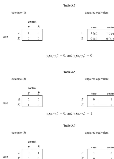
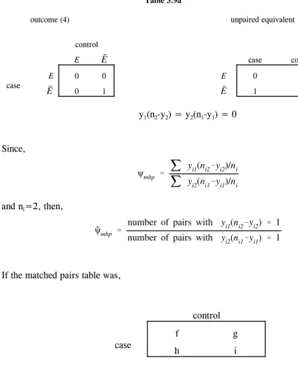
IV. ANALYSIS OF MATCHED PAIRS (ONE CASE AND ONE

CONTROL)

(9)

B. TESTING THE EQUALITY OF MARGINAL DISTRIBUTIONS

V. STATISTICAL ANALYSIS OF CLUSTERED BINARY DATA

A. TESTING HOMOGENEITY

B. INFERENCE ON THE COMMON ODDS RATIO

VI. MEASURE OF INTERCLINICIAN AGREEMENT FOR

CATEGORICAL DATA

A. AGREEMENT IN 2x2 TABLES (TWO CLINICIANS AND TWO CATEGORIES)

B. CONFIDENCE INTERVAL ON KAPPA IN 2x2 TABLE C. AGREEMENT BETWEEN TWO RATERS WITH MULTIPLE

A. GROUP TESTING

B. EVALUATING THE PERFORMANCE OF MEDICAL SCREENING TESTS IN THE ABSENCE OF A GOLD STANDARD (Latent Class Models)

Chapter 4

LOGISTIC REGRESSION

I. INTRODUCTION

II. THE LOGISTIC TRANSFORMATION

III. CODING CATEGORICAL EXPLANATORY VARIABLES AND INTERPRETATION OF COEFFICIENTS

IV. INTERACTION AND CONFOUNDING

V. THE GOODNESS OF FIT AND MODEL COMPARISONS

A. PEARSON'S _!2_{- STATISTIC}

B. THE LIKELIHOOD RATIO CRITERION (Deviance)

VI. LOGISTIC REGRESSION OF CLUSTERED BINARY DATA

A. INTRODUCTION

B. INTRACLUSTER EFFECTS

(10)

D. FULL LIKELIHOOD MODELS

E. ESTIMATING EQUATIONS APPROACH

VII. LOGISTIC REGRESSION FOR CASE-CONTROL STUDIES A. COHORT VERSUS CASE-CONTROL MODELS B. MATCHED ANALYSIS

C. CONDITIONAL LIKELIHOOD

D. FITTING MATCHED CASE-CONTROL STUDY DATA IN SAS

Chapter 5

THE ANALYSIS OF TIME SERIES

I. INTRODUCTION

A. SIMPLE DESCRIPTIVE METHODS

II. FUNDAMENTAL CONCEPTS IN THE ANALYSIS OF TIME SERIES

A. STOCHASTIC PROCESSES B. STATIONARY SERIES

C. THE AUTOCOVARIANCE AND AUTOCORRELATION FUNCTIONS

III. MODELS FOR STATIONARY TIME SERIES A. AUTOREGRESSIVE PROCESSES B. MOVING AVERAGE PROCESSES

C. THE MIXED AUTOREGRESSIVE MOVING AVERAGE PROCESS

IV. MODELS FOR NONSTATIONARY TIME SERIES

A. NONSTATIONARITY IN THE MEAN B. DIFFERENCING

C. ARIMA MODELS

D. NONSTATIONARITY IN THE VARIANCE

V. MODEL SPECIFICATION AND PARAMETER

ESTIMATION

A. SPECIFICATION B. ESTIMATION

VI. FORECASTING

VII. MODELLING SEASONALITY WITH ARIMA: The condemnation rate series revisited

VIII. THE ONE-WAY AND TWO-WAY ANALYSIS OF VARIANCE WITH TIME SERIES DATA

A. INTRODUCTION

(11)

Chapter 6

REPEATED MEASURES ANALYSIS

I. INTRODUCTION

II. EXAMPLES

A. "EFFECT OF MYCOBACTERIUM INOCULATION ON WEIGHT" B. VARIATION IN TEENAGE PREGNANCY RATES (TAPR)

IN CANADA

III. METHODS FOR THE ANALYSIS OF REPEATED MEASURES EXPERIMENTS

A. BASIC MODELS

B. HYPOTHESIS TESTING

C. RECOMMENDED ANALYSIS FOR EXAMPLE A D. RECOMMENDED ANALYSIS FOR EXAMPLE B

IV. MISSING OBSERVATIONS

V. MIXED LINEAR REGRESSION MODELS

A. FORMULATION OF THE MODELS

B. MAXIMUM LIKELIHOOD (ML) AND RESTRICTED

MAXIMUM LIKELIHOOD (REML) ESTIMATION

C. MODEL SELECTION

VI. THE GENERALIZED ESTIMATING EQUATIONS APPROACH

Chapter 7

SURVIVAL DATA ANALYSIS

I. INTRODUCTION

II. EXAMPLES

A. VENTILATING TUBE DATA B. CYSTIC OVARY DATA C. BREAST CANCER DATA

III. THE ANALYSIS OF SURVIVAL DATA A. NON-PARAMETRIC METHODS

B. NON-PARAMETRIC SURVIVAL COMPARISONS BETWEEN GROUPS

C. PARAMETRIC METHODS D. SEMI-PARAMETRIC METHODS

IV. CORRELATED SURVIVAL DATA

A. MARGINAL METHODS B. FRAILTY MODELS

(12)

Chapter 1

COMPARING GROUP MEANS WHEN THE STANDARD ASSUMPTIONS ARE VIOLATED

I. INTRODUCTION

A great deal of statistical experiments are conducted so as to compare two or more groups. It is understood that the word 'group' is a generic term used by statisticians to label and distinguish the individuals who share a set of experimental conditions. For example, diets, breeds, age intervals, methods of evaluations etc. are groups. In this chapter we will be concerned with comparing group means. When we have two groups, that is when we are concerned with comparing two means µ₁, and µ2, the familiar Student t-statistic is the tool that is commonly used by most data analysts. If we are interested in comparing several group means; that is if the null hypothesis is H0:µ1=µ2=...=µk, a problem known as the "Analysis of Variance", we use the F-ratio to seek the evidence in the data and see whether it is sufficient to justify the above hypothesis.

In performing an "Analysis of Variance" (ANOVA) experiment, we are always reminded of three basic assumptions:

Assumption (1): That the observations in each group are a random sample from a normally distributed population with mean µi and variance σi

2_{(i=1,2,...k).}

Assumption (2): The variances σ₁2,...σ_k2 are all equal. This is known as the variance homogeneity assumption.

Assumption (3): The observations within each group should be independent.

The following sections will address the effect of the violation of each of these three assumptions on the ANOVA procedure, how it manifests itself, and possible corrective steps which can be taken.

A. NON-NORMALITY

(13)

b₁ _! 1

n !

n

j!1

(y_j_"y¯)3 _/ 1

n !

n

j!1

(y_j_"y¯)2 3/2

b₂ _! 1

n !

n

j!1

(y_j_"y¯)4 / 1

n !

n

j!1

(y_j_"y¯)2 2

.

u _! b₁ (n#1)(n#3)

6(n_"2) 1/2

,

we need some notation to facilitate the presentation. Let yij denote the jth observation in the ith group, where j=1,2,...ni and i=1,2,...k. Moreover suppose that yij = µi+eij, where it is assumed that e_ij are identically, independently and normally distributed random variables with E(e_ij)=0 and variance (eij)=σ

2_{(or e}

ij! iid N(0,σ

2_{)). Hence, y}

ij! iid N (µi,σ

2_{), and the assumption of normality of the data} yij needs to be verified before using the ANOVA F-statistic.

Miller (1986, p.82) recommended that a test of normality should be performed for each group. One should avoid omnibus tests that utilize the combined groups such as a combined goodness-of-fit

χ2_{test or a multiple sample Kolmogorov-Smirnov. A review of these tests is given in D'Agostino and} Stephens (1986, chapter 9). They showed that the χ2 test and Kolmogorov test have poor power properties and should not be used when testing for normality.

Unfortunately, the preceeding results are not widely known to nonstatisticians. Major statistical packages, such as SAS, perform the Shapiro-Wilk, W test for group size up to 50. For larger group size, SAS provides us with the poor power Kolmogorov test. This package also produces measures of skewness and kurtosis, though strictly speaking these are not the actual measures of skewness !b1 and kurtosis b2 defined as

In a recent article by D'Agostino et al. (1990) the relationship between b₁ and b₂ and the measures of skewness and kurtosis produced by SAS is established. Also provided is a simple SAS macro which produces an excellent, informative analysis for investigating normality. They recommended that, as descriptive statistics, values of !b1 and b2 close to 0 and 3 respectively, indicate normality. More precisely, the expected values of these are 0 and 3(n-1)/(n+1) under normality.

To test for skewness, the null hypothesis, H0: underlying population is normal is tested as follows (D'Agostino and Pearson 1973):

(14)

β₂( b₁) _! 3(n

2_#₂₇_n_"₇₀₎₍_n_#₁₎₍_n_#₃₎ (n_"2)(n_#5)(n_#7)(n_#9)

w2 _!"1 _# 2β₂( b₁)_"1 1/2 ,

δ _! (ln w)"1/2 _, _and _α _! _2/(_w2_"₁₎ 1/2 _.

Z( b₁) _! δ ln (u/α _# "(u/α)2 _#₁#1/2_{) .}

E(b₂) _! 3(n"1)

n_#1

Var(b₂) _! 24n(n"2)(n"3) (n_#1)2(n_#3)(n_#5)

x _! (b2"E(b2)) Var(b₂)

3. Compute

Z(_!b₁) has approximately standard normal distribution, under the null hypothesis.

To test for kurtosis, a two-sided test (for β2"3) or one-sided test (for β2>3 or β2<3) can be constructed:

1. Compute b2 from the data.

2. Compute

and

(15)

β₁(b₂) _! 6(n

2_"₅_n_#₂₎ (n_#7)(n_#9)

6(n_#3)(n_#5)

n(n_"2)(n_"3)

A _! 6_# 8

β₁(b₂) 2

β₁(b₂) #

1_# 4

β₁(b₂)

Z(b₂) _! 2/(9A)"1/2 ₁_" 2 9A "

1_"2/A

1#x 2/(A_"4) 1/3

.

K2 _! (Z( b₁))2 # (Z(b₂))2 (1.1)

b₁ _! (n"2) n(n_"1)

g₁ _(1.2)

b₂ ! (n"2)(n"3)

(n_#1)(n_"1) g2 #

3(n_"1)

n_#1 . (1.3)

4. Compute

and

5. Compute

Z(b2) has approximately standard normal distribution, under the null hypothesis.

D'Agostino and Pearson (1973) constructed a test based on both _!b₁ and b₂ to test for skewness and kurtosis. This test is given by

and has approximately a chi-square distribution with 2 degrees of freedom.

For routine evaluation of the statistic K2, the SAS package produces measures of skewness (g₁) and kurtosis (g₂) that are different from _!b₁ and b₂. After obtaining g₁ and g₂ from PROC UNIVARIATE in SAS, we evaluate !b1 as

and

One then should proceed to compute Z(!b1) and Z(!b2) and hence K 2_. Note that when n is large, _!b₁# g₂ and b₂# g₂.

(16)

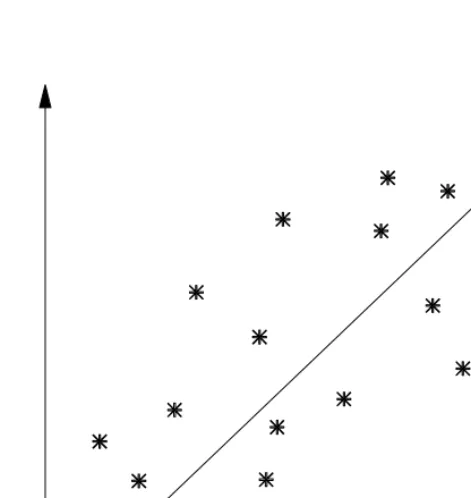
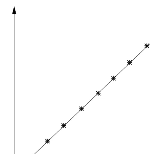
of the data. A very effective technique is the empirical quantile-quantile plot (Wilk and Gnanadesikan, 1968). It is constructed by plotting the quantiles of the empirical distribution against the corresponding quantiles of the normal distribution. If the quantiles plot is a straight line, it indicates that the data is drawn from a normal population.

A good complete normality test would consist of the use of the statistic K2_{and the normal} quantile plot.

Note that if the empirical quantile-quantile plot follows a straight line one can be certain, to some extent, that the data is drawn from a normal population. Moreover, the quantile-quantile plot provides a succinct summary of the data. For example if the plot is curved this may suggest that a logarithmic transformation of the data points could bring them closer to normality. The plot also provides us with a useful tool for detecting outlying observations.

In addition to the quantile-quantile plot, a box plot (Tukey, 1977) should be provided for the data. In the box plot the 75th and 25th percentiles of the data are portrayed by the top and bottom of a rectangle, and the median is portrayed by a horizontal line segment within the rectangle. Dashed lines extend from the ends of the box to the adjacent values which are defined as follows. First the inter-quantile range IQR is computed as:

IQR = 75th percentile - 25th percentile.

The upper adjacent value is defined to be the largest observation that is less than or equal to the 75th percentile plus (1.5) IQR. The lower adjacent value is defined to be the smallest observation that is greater or equal to the 25th percentile minus (1.5) IQR. If any data point falls outside the range of the two adjacent values, it is called an outside value (not necessarily an outlier) and is plotted as an individual point.

The box-plot displays certain characteristics of the data. The median shows the center of the distribution; and the lengths of the dashed lines relative to the box show how far the tails of the distribution extend. The individual outside values give us the opportunity to examine them more closely and subsequently identify them as possible outliers.

Example 1.1 120 observations representing the average milk production per day/herd in kilograms were collected from 10 Ontario farms (see; Appendix 1). All plots are produced by SAS.

(17)

Table 1.1

Output of the SAS UNIVARIATE PROCEDURE on the Original Data.

Variable = Milk

Moments

N Mean Std Dev Skewness USS CV T:Mean=0 Sgn Rank Num ^= 0 W:Normal

120 26.74183 3.705186 -0.54127 87448.76 13.85539 79.06274 3630 120 0.970445

Sum Wgts Sum Variance Kurtosis CSS Std Mean Prob>|T| Prob>|S|

Prob<W

120 3209.02 13.7284 0.345688 1633.68 0.338236 0.001 0.001

0.1038

The result of D'Agostino et al (1990) procedure is summarized in Table 1.2.

Table 1.2

Results of a Normality Test on the Original Data Using a SAS Macro Written by D'Agostino et al (1990)

SKEWNESS g1=-0.54127 b1=-0.53448 Z(!b1)=-2.39068 p=0.0168 KURTOSIS g₂=0.34569 b₂=3.28186 Z(_!b₂)=0.90171 p=0.3672

OMNIBUS TEST K2_{=6.52846 (against chisq 2df)} _p=0.0382

The value of the omnibus test (6.528), when compared to a chi squared value with 2 degrees of freedom (5.84) is found to be significant. Thus, based on this test, we can say that the data are not normally distributed.

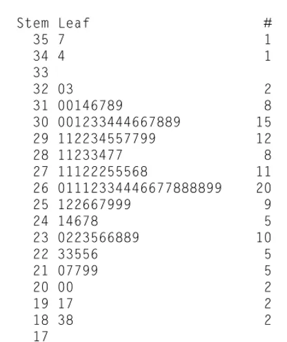
In attempting to improve the normality of the data, it was found that the best results were obtained through squaring the milk yield values. This solved the skewness problem and resulted in a non significant K2_{value (}_{Table 1.3}_{). Combined with the normal probability plot (}_{Figure 1.3}₎ produced by the D'Agostino et al. (1990) macro, one can see that the data has been normalized.

Table 1.3

Results of a Normality Test on the Transformed Data (Milk2

)

SKEWNESS g1 = -0.11814 b1 = 0.11666 Z = -0.54876 p = 0.5832 KURTOSIS g2 = -0.03602 b2 = 2.91587 Z = 0.00295 p = 0.9976

OMNIBUS TEST

(18)

Stem Leaf # Boxplot

35 7 1 |

34 4 1 |

33 |

32 03 2 |

31 00146789 8 |

30 001233444667889 15 |

29 112234557799 12 +---+

28 11233477 8 | |

27 11122255568 11 | |

26 01112334446677888899 20 *--+--*

25 122667999 9 | |

24 14678 5 +---+

23 0223566889 10 |

22 33556 5 |

21 07799 5 |

20 00 2 |

19 17 2 |

18 38 2 |

17

16 3 1 0

15 4 1 0

(19)

1388.79 + | | | SQMILK |

| * |

| | 1196.95 +

| * |

| | | |

| * | ** 1005.12 + *** | * | *** | ** | ** | ** | ** | *** | * 813.28 + * | ** | * | ** | ** | *** | *** | ** | * 621.45 + ** | * | * | ** | ** | ** | * | ** | * 429.61 +

| * | * | * | * * |

| |

| * 237.78 + *

(20)

B _! M / C (1.4)

M _! ν log s2 _" !

k

i!1

ν_i log s_i2 ,

ν_i _! n_i_"1 , ν _! !

k

i!1

ν_i , s2 _! 1

ν !

k

i!1

ν_i s_i2 ,

s_i2 _! 1

!_i ! n_i

j!1

(y_ij_"y_i)2 , y_i _! 1

n_i !

n_i

j!1

y_ij

C _! 1_# 1

3(k"1) !

k

i!1 1

ν_i "

1

ν .

B. HETEROGENEITY OF VARIANCES

The effect of unequal variances on the F-test of the ANOVA problem had been investigated by Box (1954a). He showed that in balanced experiments (i.e. when n1=n2=...=nk) the effect

of heterogeneity is not too serious. When we have unbalanced experiments then the effect can be more serious, particularly if the large "i2 are associated with the small ni. The recommendation

is to balance the experiment whenever possible, for then unequal variances have the least effect.

Detecting heterogeneity or testing the hypothesis H0:"1 2_="

2

2_=...=" k

2_{, is a problem that}

has applications in the field of measurement errors, particularly reproducibility and reliability studies as will be seen in the next chapter. In this section we introduce some of the widely used tests of heterogeneity.

1. Bartlett's Test

Bartlett (1937) modified the likelihood ratio statistic on H0:"12="22=..."k2 by introducing

a test statistic widely known as Bartlett's test on homogeneity of variances. This test statistic is given as

where

(21)

L_ij _! $ y_ij_"y¯_i $ , (i_!1,2,...k) .

WL _! 1

k_"1 !

k

i!1

w_i y¯_i _" y 2

c₁ (1.5)

One of the disadvantages of Bartlett's test is that it is quite sensitive to departure from normality. In fact, if the distributions from which we sample are not normal, this test can have an actual size several times larger than its nominal level of significance.

2. Levene's Test (1960)

The second test was proposed by Levene (1960). It entails doing a one-way ANOVA on the variables

If the F-test is significant, homogeneity of the variances is in doubt. Brown and Forsythe (1974a) conducted extensive simulation studies to compare between tests on homogeneity of variances and reported the following.

(i) If the data are nearly normal, as evidenced by the previously outlined test of normality, then we should use Bartlett's test which is equally suitable for balanced and unbalanced data.

(ii) If the data are not normal, Levene's test should be used. Moreover, if during the step of detecting normality we find that the value of !b1 is large, that is if the data tend to be very skewed, then Levene's test can be improved by replacing ¯yi by ˜yi, where ˜yi is the median of the ith group. Therefore ˜Lij = $yij-˜yi$, and an ANOVA is done on ˜Lij. The conclusion would be either to accept or reject H₀:σ₁2_=...=_σ

k

2_{. If the hypothesis is accepted, then the main hypothesis of equality of several means} can be tested using the familiar ANOVA.

If the heterogeneity of variances is established, then it is possible to take remedial action by employing transformation on the data. As a general guideline in finding an appropriate transformation, first plot the k pairs (¯yi, si

2_{) i=1,2...k as a means to detect the nature of the} relation-ship between ¯yi and si

2_{. For example if the plot exhibits a relationship that is approximately linear we} may try log yij. If the plot shows a curved relationship we suggest the square root transformation. Whatever transformation is selected, it is important to test the variance heterogeneity on the tranformed data to ascertain if the transformation has in fact stabilized the variance.

If attempts to stabilize the variances through transformation are unsuccessful, several approximately valid procedures to compare between group means in the presence of variance heterogeneity, have been proposed. The most commonly used are:

(22)

c₁ _! 1_# 2(k"1) (k2_"1) !

k

i!1

(n_i_"1)"1 ₁_"wi

w

2

w_i _! n_i/s_i2 , w _! !

k

i!1

w_i , and

y _! !

k

i!1

w_i y_i / w

f₁ _! 3

(k2"1) !

k

i!1

(n_i_"1)"1 ₁_"wi

w

2"1

(1.6)

BF _! !

k

i!1

n_i y_i_"y2 / c₂ (1.7)

c₂ _! !

k

i!1

1"ni

N s

2

i

y _! 1

N !

k

i!1 !

n_i

j!1

y_ij , and N _! n₁_#n₂_#..._#n_k .

f₂ _! !

k

i!1

(n_i_"1)"1 a_i2

"1

When all population means are equal (even if the variances are unequal), WL is approximately distributed as an F-statistic with k-1 and f1 degrees of freedom,

where

4. Brown and Forsythe Statistic (1974b) for Testing Equality of Group Means:

where

(23)

a_i _! 1"ni

N s

2

i / c2

G _! !

k

i!1

w_i (y_i_"µ)2 _(1.8)

! !

k

i!1

w_i y¯2_i _" (!

k

i!1

w_i y¯_i)2 _/ _w _(1.9)

ˆ

G _! !

k

i!1

w_i (y_i_"y)2

Remarks:

1. The approximations WL and BF are valid when each group has at least 10 observations and are not unreasonable for WL when the group size is as small as five observations per group.

2. The choice between WL and BF depends upon whether extreme means are thought to have extreme variance in which case BF should be used. If extreme means have smaller variance, then WL is preferred. Considering the structure of BF, Brown and Forsythe recommend the use of their statistic if some sample variances appear unusually low.

5. Cochran's (1937) Method of Weighting for Testing Equality of Group Means:

To test the hypothesis H0:µ1=µ2=...=µk=µ, where µ is a specified value, Cochran suggested the weighted sum of squares

as a test statistic on the above hypothesis.

The quantity G follows (approximately) a χ_k2 distribution. However, if we do not wish to specify the value of µ it can be replaced by !y and then G becomes

It can be shown that, under the null hypothesis of equality of means, !_{is approximately distributed}

as χ2k-1; the loss of 1 degree of freedom is due to the replacement by µ by !

y. Large values of ˆG

indicate evidence against the equality of the means.

(24)

Table 1.4

Summary Statistics for Each of the Ten Farms

Farm Mean ni Std. Dev. si2

1 30.446 12 1.7480 3.0555

2 29.041 12 2.9314 8.5931

3 24.108 12 3.3302 11.0902

4 27.961 12 3.2875 10.8077

5 29.235 12 1.7646 3.1138

6 27.533 12 2.1148 4.4724

7 28.427 12 1.9874 3.9498

8 24.473 12 1.8912 3.5766

9 24.892 12 1.7900 3.2041

10 21.303 12 3.8132 14.5405

The value of the Bartlett's statistic is B=18.67, and from the table of chi-square at 9 degrees of freedom, the p-value 0.028. Therefore there is evidence of variance heterogeneity.%

However, after employing the square transformation on the data (see summary statistics in Table 1.5) the Bartlett's statistic is B=14.62 with p-value 0.102.%

Hence, by squaring the data we achieve two objectives; first the data were transformed to normality; second, the variances were stabilized.

Table 1.5

Summary Statistics on the Transformed Data (Milk2_{) for Each of the Ten Farms}

Farm Mean ni Std. Dev. s2

1 929.75 12 109.020 11885.36

2 851.25 12 160.810 25.859.86

3 591.34 12 158.850 25233.32

4 791.72 12 195.020 38032.80

5 857.54 12 102.630 10532.92

6 762.18 12 116.020 13460.64

7 811.74 12 113.140 12800.66

8 602.22 12 92.774 8607.02

9 622.53 12 88.385 7811.91

(25)

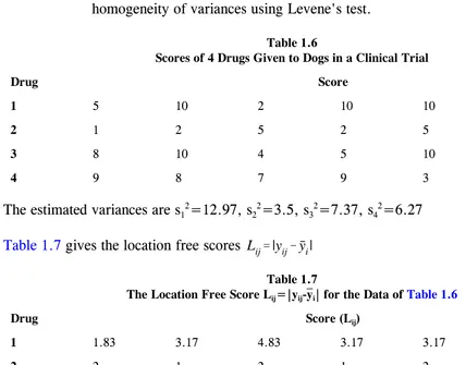
Example 1.3 The following data are the results of a clinical trial involving 4 groups of dogs assigned at random to each of 4 therapeutic drugs believed to treat compulsive behaviour. The scores given in Table 1.6 are measures of the severity of the disorder after 21 days of treatment. Before comparing the mean scores, we test the homogeneity of variances using Levene's test.

Table 1.6

Scores of 4 Drugs Given to Dogs in a Clinical Trial

Drug Score

1 5 10 2 10 10 4

2 1 2 5 2 5

3 8 10 4 5 10 10

4 9 8 7 9 3 10

The estimated variances are s12=12.97, s22=3.5, s32=7.37, s42=6.27

Table 1.7 gives the location free scores L_ij_!|y_ij_"y¯_i|

Table 1.7

The Location Free Score Lij= $$$$yij-¯yi $$$$ for the Data of Table 1.6

Drug Score (Lij)

1 1.83 3.17 4.83 3.17 3.17 2.83

2 2 1 2 1 2

3 0.17 2.170 3.83 2.13 2.17 2.17

4 1.33 0.33 0.67 1.33 4.67 2.33

In Table 1.8 we provide the result of the ANOVA on Lij; the F-statistic = 2.11 with P-value =

0.133. This indicates that there is no significant difference between the variances of the 4 groups even though visually the estimated variances seem quite different from each other.

Table 1.8 ANOVA of Lij

Source df Sum Square Mean Square F Value Pr>F

Model 3 8.47824 2.82608 2.11 0.1326

Error 19 25.4350 1.33868

(26)

var (y) _! σ 2

n 1#2ρ ,

Levene's test could not detect this heterogeneity because the sample sizes and the number of groups are small. This lack of power is a common feature of many nonparametric tests such as Levene's.

C. NON-INDEPENDENCE

A fundamental assumption in the analysis of group means is that the samples must be independent, as are the observations within each sample. For now, we shall analyze the effect of within sample dependency with emphasis on the assumption that the samples or the groups are independent of each other.

Two types of dependency and their effect on the problem of comparing means will be discussed in this section. The first type is caused by a sequence effect. The observations in each group may be taken serially over time in which case observations that are separated by shorter time intervals may be correlated because the experimental conditions are not expected to change, or because the present observation may directly affect the succeeding one. The second type of correlation is caused by blocking effect. The ni data points yi1...y_ini may have been collected as

clusters. For example the y's may be collected from litters of animals, or from "herds". The possibility that animals or subjects belonging to the same cluster may respond in a similar manner (herd or cluster effect) creates a correlation that should be accounted for. The cluster effect can be significantly large if there are positive correlations between animals within clusters or if there is a trend between clusters. This within herd correlation is known as the intracluster correlation and will be denoted by #.

Before we examine the effect of serial correlation on comparing group means, we shall review its effect on the problem of testing one mean, that is its effect on the t-statistic.

The simplest time sequence effect is of a serial correlation of lag 1. Higher order lags are discussed in Albers (1978). Denoting y1...yn as the sample values drawn from a population with

mean µ and variance "2_{, we assume that}

Cov ( yi ,yi+j ) = ρjσ2 j=0,1

$₀ _otherwise

(27)

ˆ

σ2 _! s2 _! 1

n_"1 !

n

i!1

(y_i _" y)2

ˆ

ρ _! 1

n_"1 !

n"1

i!1

(y_i _"y) (y_i_#₁ _" y) / s2 .

(1.10)

v_i _! varˆ (y_i) _! s 2

i

n_i 1 # 2ˆρi

and since the parameters "2_{and # are unknown we may replace them by their moment estimators}

and

Note that the var (¯y) in the presence of serial correlation is inflated by the factor d=1+2ρ. This means that if we ignore the effect of ρ the variance of the sample mean would be under estimated. The t-statistic thus becomes

t _! n (y"µ) s 1_#2ˆρ

. _(1.11)

To illustrate the unpleasant effect of ˆρ on the p-value, let us consider the following hypothetical example. Suppose that we would like to test H0:µ=30 versus H1:¯y>30. The sample information is, ¯y=32, n=100, s=10, and ˆρ=0.30. Therefore, from equation (1.11), t=1.58, and the p-value 0.06.#

If the effect of ˆρ were ignored, then t=2.0 and the p-value 0.02.#

This means that significance will be spuriously declared if the effect of ˆρ is ignored.

Remark: It was recommended by Miller (1986) that a preliminary test of ρ=0 is unnecessary, and that it is only the size of ˆρ that is important.

We now return to the problem of comparing group means. If the observations within each group are collected in time sequence, we compute the serial correlations ˆρ_i (i=1,2,...k). Few papers researching the effect of serial correlation on the ANOVA F statistic are available.We shall report on their quantitative merits in Chapter 6, which is devoted to the analysis of repeated measurements. However, the effect of correlation can be salvaged by using the serial correlation estimates together with one of the available approximate techniques. As an illustration; let yi1,yi2,...y_ini be the observations from the ith group and let ¯yi, and si

2_{be the sample means and variances} respectively. If the data in each sample are taken serially, the serial correlation estimates are ˆρ₁

ˆ

(28)

y _! !

k

i!1

w_i y_i / w , w _! !

k

i!1

w_i .

ˆ

G _! !

k

i!1

w_i (y_i _" y)2 then wi=vi

-1_{can be used to construct a pooled estimate for the group means under the hypothesis} H0:µ1=...=µk. This estimate is

The hypothesis is thus rejected for values of

exceeding χ2k-1 at the α-level of significance.

To account for the effect of intraclass correlation a similar approach may be followed. Procedures for estimating the intraclass correlation will be discussed in Chapter 2.

Example 1.4 The data are the average milk production per cow per day, in kilograms, for 3 herds over a period of 10 months (Table 19). For illustrative purposes we would like to use Cochran's statistic ! to compare between the herd means. Because the data were collected in serial order one should account for the effect of the serial correlation.

Table 1.9

Milk Production Per Cow Per Day in Kilograms for 3 Herds Over a Period of 10 Months.

Farm Months

1 2 3 4 5 6 7 8 9 10

1 25.1 23.7 24.5 21 19 29.7 28.3 27.3 25.4 24.2

2 23.2 24.2 22.8 22.8 20.2 21.7 24.8 25.9 25.9 25.9

3 21.8 22.0 22.1 19 18 17 24 24 25 19

The estimated variances and serial correlations of the 3 herds are: s12=9.27, s22=3.41, s32=6.95,

ˆ

#₁=0.275, ˆ#₂=.593, and ˆ#₃=0.26. Therefore v1=1.36, v2=0.75, and v3=1.06. Since =6.13,Gˆ

(29)

Remarks on SAS programming:

We can test the homogeneity of variances (HOVTEST) of the groups defined by the MEANS effect within PROC GLM. This can be done using either Bartlett’s test (1.4) or Levene’s test

L

ij

by adding

the following options to the MEANS statement :

MEANS group | HOVTEST = BARTLETT; or

(30)

Chapter 2

STATISTICAL ANALYSIS OF MEASUREMENTS RELIABILITY

"The case of interval scale measurements"

I. INTRODUCTION

The verification of scientific hypotheses is only possible by the process of experimentation, which in turn often requires the availability of suitable instruments to measure materials of interest with high precision.

The concepts of "precision" and "accuracy" are often misunderstood. To correctly understand such concepts, modern statistics provides a quantitative technology for experimental science by first defining what is meant by these two terms, and second, developing the appropriate statistical methods for estimating indices of accuracy of such measurements. The quality of measuring devices is often described by reliability, repeatability (reproducibility) and generalizability, so the accuracy of the device is obviously an integral part of the experimental protocol.

The reader should be aware that the term "device" refers to the means by which the measurements are made, such as the instrument, the clinician or the interviewer. In medical research, terms such as patient reliability, interclinician agreement, and repeatability are synonymous with a group of statistical estimators which are used as indices of the accuracy and precision of biomedical measurements. To conduct a study which would measure the reliability of a device, the common approach is to assume that each measurement consists of two parts, the true unknown level of the characteristic measured (blood pressure, arm girth, weight etc.) plus an error of measurement. In practice it is important to know how large or small the error variance, or the imprecision, is in relation to the variance of the characteristic being measured. This relationship between variances lays the ground rules for assessing reliability. For example, the ratio of the error variance to the sum of the error variance plus the variance of the characteristic gives, under certain conditions, a special estimate of reliability which is widely known as the intraclass correlation (denoted by !). There are numerous versions of the intraclass correlation, the appropriate form for the specific situation being defined by the conceptual intent of the reliability study.

(31)

y_ij _! µ _" g_i _" e_ij _(2.1)

ρ _! cov(yij,yil)

var(y_ij), var(y_il)

! σ

2 g

σ2_g _" σ2_e .

II. MODELS FOR RELIABILITY STUDIES

An often encountered study for estimating ! assumes that each of a random sample of k patients is evaluated by n clinicians.

Three different cases of this kind of study will be investigated. For each of these, a description of the specific mathematical models that are constructed to evaluate the reliability of measurements is given.

A. CASE 1: THE ONE-WAY RANDOM EFFECTS MODEL

This model has each patient or subject being measured (evaluated) by the same device.

Let yij denote the jth rating on the ith patient (i=1,2,...k ; j=1,2,...n). It is quite possible

that each patient need not be measured a fixed number of times n, in which case we would have unbalanced data where j=1,2,...ni. In general we assume the following model for yij

where µ is the overall population mean of the measurements; gi is the true score of the ith patient;

and eij is the residual error. It is assumed that gi is normally distributed with mean zero and

variance "_g2_{and independent of e}

ij. The error eij is also assumed to be normally distributed with

mean zero and variance "_e2_{. The variance of y}

ij is then given by "y2 = "g2+"e2.

Since

Cov (yij, yil) = "g

2_{i=1,2,...k ; j}_!_l=1,2,...n i

the correlation between any pair of measurements on the same patient is

This model is known as the components of variance model, since interest is often focused on estimation of the variance components "_g2_and_"

e2. The ANOVA corresponding to (2.1) is shown

(32)

N _! _!

k

i!1

n_i , y_i _! 1

n_i !

n_i

j!1

y_ij , and y _! 1

N !

k

i !

n_i

j

y_ij ,

n_o _! 1

k_#1 N # !

k

i!1

n_i2 / N .

r₁ ! σˆ2_g / ( ˆσ_g2 _" σˆ2_e) ! MSB#MSW

MSB_"(n_o_#1)MSW . (2.2)

and

Since unbiased estimators of "_e2_and_" g

2_{are given respectively by ˆ}_" e

2_{= MSW and}

ˆ

"_g2_{= (MSB-MSW)/n}

o, it is natural to define the ANOVA estimator of ! as

This estimator of reliability is biased.

Table 2.1

The ANOVA Table Under the One-way Random Effects Model.

Source of Variation

D.F. S.S. M.S. E(M.S.)

Between Patients

K-1

SSB_!_!

K

i!1

n_i(y_i_#y)2 MSB=SSB/(K-1) (1+(n0-1)!)"y2

Within Patients

N-K

SSW_!_!

K

i!1 ! n_i

j!1

(y_ij_#y_i)2 MSW=SSW/(N-K) (1-!)"y2

Total N-1

SST_!_!

K

i!1 ! n_i

j!1

(y_ij_#y)2

(33)

v(r₁) ! 2(1#ρ)2

n_o2

[1"ρ(n_o#1)]2

N#k "

(k#1)(1#ρ)[1"ρ(2n_o#1)]"ρ2λ(n_i)

(k#1)2 (2.3)

λ(n_i) _! _!n_i2 _# 2N#1 _!n_i3 _" N#2 _!n_i2 2 .

r₁ _# Z_α

/2 vˆ(r1) , r1 " Zα/2 vˆ(r1)

y_ij _! µ " g_i _" c_j _" e_ij . _(2.4)

var(y_ij) _! σ2_g _" σ2_c _" σ2_e , where

Donner and Wells (1985) showed that an accurate approximation of the confidence limits on ! for moderately large k, is given by:

where ˆv(r1) is defined in (2.3), with r1 replacing !, and Z#/2 is the two-sided critical value of the

standard normal distribution corresponding to the #-level.

Note that the results of this section apply only to the estimate of reliability obtained from the one-way random effects model.

B. CASE 2: THE TWO-WAY RANDOM EFFECTS MODEL

In this model, a random sample of n clinicians is selected from a larger population and each clinician evaluates each patient.

When the n raters, clinicians or devices that took part in the reliability study are a sample from a larger population, the one-way random effects model should be extended to include a rater's effect, so that

This is the so-called two-way random effects model, where the quantity cj, which characterizes

the additive effect of a randomly selected rater, is assumed to vary normally about a mean of zero with variance "_c2_{. The three random variables g,c, and e are assumed mutually independent. The}

variance of yij is

and the covariance between two measurements on the same patient, taken by the lth_{and j}th_raters

(34)

R ! σ 2 g σ2_g " σ2_c " σ2_e

. _(2.5)

n_!(¯y_i_.#y¯)2

σ2_e"nσ2_g σ2_e"nσ2_g

k_!(¯y_._j#y¯)2

σ2e"kσ 2

c _σ2

e"

k

n#1!

n i!1

d_i2

σ2_e σ2_e

! !(y_ij#y¯)2

ˆ

σ2_g ! PMS#MSW

n

ˆ

σ2_c ! CMS#MSW

k

Hence the intraclass correlation to be used as an appropriate measure of reliability under this model is,

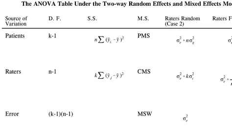
Table 2.2

The ANOVA Table Under the Two-way Random Effects and Mixed Effects Models

Source of

Variation D. F. S.S. M.S. Raters Random(Case 2) Raters Fixed (Case 3)

Patients k-1 PMS

Raters n-1 CMS

Error (k-1)(n-1) MSW

Total

The unbiased variance components estimates of "g2, "c2, and "e2 are given respectively as

(35)

r₂ _! k(PMS#MSW)

k(PMS) " n(CMS) " (nk_#n_#k)MSW (2.6)

y_ij _! µ _" g_i _" d_j _"e_ij _(2.7)

! n

t!1

d_t _! 0 .

r₃ ! k(PMS#MSW)

k(PMS) _" (n_#1)CMS _" (n_#1)(k_#1)MSW (2.8)

An estimator of reliability is then

a formula that was derived by Bartko (1966).

C. CASE 3: THE TWO-WAY MIXED EFFECTS MODEL

What typifies this model is that each patient is measured by each of the same n raters, who are the only available raters. Furthermore, under this model, the raters taking part in the study are the only raters about whom inferences will be made. In the terminology of the analysis of variance, the raters effect is assumed fixed. The main distinction between Case 2 (where clinicians are considered random) and Case 3 (where clinicians are considered fixed) is that under Case 2 we wish to generalize the findings to other raters within a larger group of raters, whereas in the Case 3 situation we are only interested in the group that took part in the study.

Following Fleiss (1986), yij is written as

Here, d1, d2,...dn are no longer random, rather they are assumed to be a set of fixed constants, and

The assumptions on gi and eij are the same as those of Cases 1 and 2. The ANOVA for this case

is provided by Table 2.2.

Under this model, the appropriate measure of reliability from Fleiss (1986), is given as

Fleiss (1986) describes the following sequential approach to estimating r3.

1- Test for clinician to clinician variation to see if clinicians differ significantly from one another. To test this hypothesis (H0: d1 = d2 = ..=dn = 0) one would compare the ratio

(36)

L _! y_.j _# 1

n#1 (y.1 "...y.j#1 " y.j"1 "..." y.n)

SE(L) _! n MSW

k(n_#1 ) 1/2

.

estimate the reliability using (equation 2.8). If F>F(n-1),(n-1)(k-1),# then the null hypothesis is rejected indicating that differential measurement bias exists.

2- When the above hypothesis is rejected, the clinician or the rater responsible for most of the significance of the differences among the raters should be determined. There is no doubt that the estimated reliability will be higher if this rater is removed.

For example, if the jth_{rater is the one in doubt we form the following contrast}

with a standard error

The jth_{rater is considered non-conforming if} _exceeds_"_t

(n-1)(k-1),#/2", in which case

L SE(L)

a recommended strategy is to drop this rater, construct a new ANOVA, and estimate reliability using (2.8).

Example 2.1

In this example, the following data will be analyzed as Case 1, Case 2 and Case 3 situations. An analytical chemist wishes to estimate with high accuracy the critical weight of chemical compound. She has 10 batches and 4 different scales. Each batch is weighed once using each of the scales. A SAS program which outlines how to create the output for the data described in Table 2.3 is given below.

Table 2.3

Critical Weights of a Chemical Component Using 4 Scales and 10 Batches.

Scale 1 2 3 4 5 6 7 8 9 10

1 55 44.5 35 45 50 37.5 50 45 65 58.5

2 56 44.5 33 45 52 40 53 50 66 56.5

3 65 62 40 37 59 50 65 50 75 65

(37)

EXAMPLE SAS PROGRAM

data chemist; input scale batch y; cards;

1 1 55 1 2 44.5 1 3 35 ....

4 7 48 4 8 47 4 9 79 4 10 57 ;

/** one way **/

proc glm data=chemist; class batch;

model y=batch; run;

/** two way - random mixed **/ proc glm data=chemist; class batch scale; model y=batch scale; run;

/** two way dropping scale 3 **/ data drop3;

set chemist;

if scale=3 then delete;

proc glm data=drop3; class batch scale; model y=batch scale; run;

As a Case 1 Situation:

Treating this as a Case 1 situation by ignoring the scale effect (which means that the order of the measurements of weights 'within' a batch does not matter), the measurement reliability is computed as r1 (see equation 2.2).

Extracts from the ANOVA tables in the SAS OUTPUT are given here:

Source DF Sum Squares Mean Square F value Pr>F

Model 9 3913.881250 434.875694 14.60 0.0001

Error 30 893.562500 29.785417

(38)

L _! y¯_.3 _# 1

3 ( ¯y.1"y¯.2"y¯.4)

SE(L) ! (n)(MSW) k(n#1)

1 2

Therefore, r1 = [434.875694 - 29.785417]/[434.875694 + (4-1)(29.785417)]

= 0.773

This is an extremely good reliability score based on the 'standard values' of comparison which are: excellent (>.75), good (.40, .75) and poor (< .40).

The ANOVA OUTPUT for the two-way random effects model that results is,

Source DF Sum Squares Mean Square F Value Pr>F

Model 12 4333.0000 361.083333 20.55 0.0001

BATCH 9 3913.88125 434.875694 24.75 0.0001

SCALE 3 419.11875 139.706250 7.95 0.0006

Error 27 474.118750 17.571991

C Total 39 4807.44375

Therefore, r2 (equation 2.6) is computed as,

r2 = 10[434.8757 - 17.572] /[(10)(434.8757) + (4-1)(139.70625) + (4-1)(10-1)(17.571991)]

= 0.796

Again, this value indicates an excellent measure of reliability, but note that the scale effect is highly significant (p=0.0006).

First of all we can test whether Scale 3 is significantly 'deviant', by using the contrast,

with standard error,

Thus, L = 7.35, SE(L) = 1.5307 and L/SE(L) = 4.802.

Since 4.802 exeeds the value of t = 2.052 (27 df at # = 0.05), there is reason to remove this 'deviant' scale.

(39)

y_ij _! µ _" g_i _" β(x_ij_#x) _" e_ij

x _! 1

N !

k

i !

n_i

j

x_ij i_!1,2,...k

j_!1,2,...n_i

N _! _!

k

i!1

n_i .

The ANOVA for the two-way mixed effects model that results is,

Source DF Sum Squares Mean Square F Value Pr>F

Model 11 2865.45833 260.496212 22.85 0.0001

BATCH 9 3913.88125 434.875694 27.79 0.0001

SCALE 2 13.9500 6.975000 0.61 0.5533

Error 18 205.216667 11.400926

C Total 29 3070.6750

Note that after removing scale 3 the F-value of the scale effect is no longer significant. In calculating r3 (equation 2.8),

r₃!10 [ 316.834#11.4009 ] / [ ( 10 ) ( 316.8343"( 3#1 ) ( 6.975 )"( 10#1 ) ( 3#1 ) ( 11.4009 ) ]!0.911

We can see that the removal of the 3rd scale has resulted in a considerable improvement in the reliability score, thus, if the scales are considered a fixed effect, it would be wise to drop the third scale.

D. COVARIATE ADJUSTMENT IN THE ONE-WAY RANDOM EFFECTS MODEL

Suppose that each of k patients is measured ni times. In a practical sense, not all

measurements on each patient are taken simultaneously, but at different time points. Since the measurements may be affected by the time point at which they are taken, one should account for the possibility of a time effect. In general, let xij denote the covariate measurement of the ith

patient at the jth_{rating. The one-way analysis of covariance random effects model is given by}

where

(40)

x_i _! 1 n_i !j

x_ij , y_i _! 1 n_i !j

y_ij

y _! 1

N !i !j

y_ij ,

E_yy _! _!

i !j

(y_ij_#y_i)2 ,

E_xx _! _!

i !j

(x_ij_#x_i)2

E_xy ! _!

i !j

(y_ij#y_i)(x_ij#x_i)

T_yy ! _!

i !j

(y_ij#y)2

T_xx _! _{! !} (x_ij_#x)2

T_xy _! _{! !}(y_ij_#y)(x_ij_#x)

Note that the assumptions for gi and eij as described in section A are still in effect. This model is

useful when an estimate of the reliability , while controlling for a potentially confoundingρ variable, such as time, is desired.

Define:

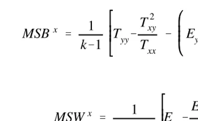
From Snedecor and Cochran (1980), the mean squares between patients and within patients, MSBx

(41)

MSBx ! 1

k_#1 Tyy#

T_xy2

T_xx # Eyy# E_xy2 E_xx

MSWx ! 1

N_#k_#1 Eyy#

E_xy2 E_xx

r₁x _! MSB

x _# _MSWx

MSBx _" (m_o_#1)MSWx

m₀ _! 1

k_#1 N#

!n_i2

N #

!n_i2(x_i_#x)2

T_xx .

Stanish and Taylor (1983) showed that the estimated intraclass correlation which controls for the confounder x is given as

where

III. COMPARING THE PRECISIONS OF TWO METHODS (GRUBBS, 1948 and SHUKLA, 1973)

In this section we will be concerned with the comparison of the performance of two measuring methods, where every sample is measured twice by both methods. This means that each patient will provide four measurements. The data layout is given in Table 2.4; the

replications from the two methods are obtained from the same patient. This produces estimates of variance components and indices of reliability that are correlated, and hence, statistical inference procedures need to be developed to deal with this situation.

Table 2.4

Measurements from Two Methods Using k Patients

Patient

1 2 . . . k

Method(1) x₁₁ x₂₁ . . . x_k1

x12 x22 . . . xk2

(42)

x_i _! xi1"xi2

2 , and yi !

y_i1_"y_i2

2 .

s_xx _! 1

k_#1 !

k

i!1

(x_i_#x)2 ,

s_yy _! 1

k_#1 !

k

i!1

(y_i_#y)2 ,

s_xy _! 1

k_#1 !

k

i!1

(x_i_#x)(y_i_#y) .

var(x_i) ! σ2 _" 1 2 σ

2 ξ

var(y_i) ! σ2 _" 1 2 σ

2 η

cov(x_i,y_i) ! σ2 .

Let x_ij_!α_"µ_i_"ξ_ij i=1,2,...k

j=1,2

y_ij_!α_"µ_i_"η_ij

where xij is the j

th_{replication on the i}th_{patient obtained by the first method and y}

ij is the j

th_replication on the ith_{patient obtained by the second method.}

Let

Here, µ_i is the effect of the ith_patient,_ξ _and _{are the measurement errors.} ij ηij

Define the estimates of the variances and covariance as,

and

Assume that µi#N(0,σ 2_),_ξ

ij#N(0,σξ

2_{), and}_η

ij#N(0,ση

2_{) and that µ}

i, ξij and ηij are mutually independent. Thus,

and

(43)

ˆ

σ2 _! s_xy

ˆ

σ2_ξ _! 2s_xx_#s_xy

ˆ

σ2_η _! 2s_yy_#s_xy .

r _! sxx#syy

s_xx_"s_yy_#2s_xy s_xx_"s_yy_"2s_xy 1/2

. _(2.9)

t_o_!r k#2

1#r2 (2.10)

If we let ui = xi + yi vi = xi - yi

then the Pearson's correlation between ui and vi is

The null hypothesis by which one can test if the two methods are equally precise is H0:σξ 2₌

σ_η2, versus the alternative H₁:σ_ξ2!σ_η2.

Shukla (1973) showed that H0 is rejected whenever

exceeds "tα/2" where tα/2 is the cut-off point found in the t-table at (1-α/2) 100% confidence, and (k-2) degrees of freedom.

Note that we can obtain estimates of reliability for method (1) and method (2) using the one-way ANOVA. Clearly such estimates are correlated since the same group of subjects is evaluated by both methods. A test of the equality of the intraclass correlations !1 and !2 must account for the correlation between ρˆ₁and ρˆ₂.

Alsawalmeh and Feldt (1994) developed a test statistic on the null hypothesis H_o:ρ₁_!ρ₂.

(44)

T_! 1#ρˆ1

1#ρˆ₂ ,

d₂! 2M

M#1, d1!

2d₂3#4d₂2

(d₂#2 )2₍_d

2#4 )V#2d 2 2

M!E1

E₂"

E₁

E₂3

V₂# C12

E₂2

E_j_! νj

ν_j_#2 #

( 1#ρ_j)

(k_#1 ) j!1,2

V_j! 2v

2

j (Cj"vj#2 )

C_j(v_j#2 )2(v_j#4 )#

2 ( 1#ρ_j)

k#1

v_j_!2 (k#1 )

1"ρ2_j

, C_j_!(k_#1 ) , C₁₂_! 2

(k_#1 )ρ 2 12, where ρˆ_j is the one way ANOVA of !_j.

The statistic T, is approximately distributed as an F random variable with d1 and d2 degrees of freedom, where,

(45)

V! E1

E₂

2

V₁

E₁2

" V2

E₂2

# 2C12

E₁E₂

ˆ

ρ₁₂_! σˆ

2

( ˆσ2_"σˆ2_ξ)( ˆσ2_"σˆ2_η 1/2

The parameter ρ₁₂ is the correlation between individual measurements x_j and y_j from the two methods. An estimate of ρ₁₂ is given by,

Unfortunately, the test is only valid when k>50.

Example 2.2 Comparing the precision of two methods:

The following data (Table 2.5) were provided by Drs. Viel and J. Allen of the Ontario Veterinary College in investigating the reliability of readings of bacterial contents from 15 samples of nasal swabs taken from 15 animals with respiratory infection.