For further information, see
www.cacr.math.uwaterloo.ca/hac
CRC Press has granted the following specific permissions for the electronic version of this
book:
Permission is granted to retrieve, print and store a single copy of this chapter for
personal use. This permission does not extend to binding multiple chapters of
the book, photocopying or producing copies for other than personal use of the
person creating the copy, or making electronic copies available for retrieval by
others without prior permission in writing from CRC Press.
Except where over-ridden by the specific permission above, the standard copyright notice
from CRC Press applies to this electronic version:
Neither this book nor any part may be reproduced or transmitted in any form or
by any means, electronic or mechanical, including photocopying, microfilming,
and recording, or by any information storage or retrieval system, without prior
permission in writing from the publisher.
The consent of CRC Press does not extend to copying for general distribution,
for promotion, for creating new works, or for resale. Specific permission must be
obtained in writing from CRC Press for such copying.
c
Chapter
4Public-Key Parameters
Contents in Brief
4.1 Introduction. . . 133
4.2 Probabilistic primality tests. . . 135
4.3 (True) Primality tests . . . 142
4.4 Prime number generation. . . 145
4.5 Irreducible polynomials overZp . . . 154
4.6 Generators and elements of high order. . . 160
4.7 Notes and further references . . . 165
4.1 Introduction
The efficient generation of public-key parameters is a prerequisite in public-key systems. A specific example is the requirement of a prime numberpto define a finite fieldZpfor use in the Diffie-Hellman key agreement protocol and its derivatives (§12.6). In this case, an element of high order inZ∗p is also required. Another example is the requirement of primespandqfor an RSA modulusn = pq(§8.2). In this case, the prime must be of sufficient size, and be “random” in the sense that the probability of any particular prime being selected must be sufficiently small to preclude an adversary from gaining advantage through optimizing a search strategy based on such probability. Prime numbers may be required to have certain additional properties, in order that they do not make the associated cryptosystems susceptible to specialized attacks. A third example is the requirement of an irreducible polynomialf(x)of degreemover the finite fieldZpfor constructing the finite fieldFpm. In this case, an element of high order inF∗pmis also required.
Chapter outline
4.1.1 Approaches to generating large prime numbers
To motivate the organization of this chapter and introduce many of the relevant concepts, the problem of generating large prime numbers is first considered. The most natural method is to generate a random numbernof appropriate size, and check if it is prime. This can be done by checking whethernis divisible by any of the prime numbers≤ √n. While more efficient methods are required in practice, to motivate further discussion consider the following approach:
1. Generate ascandidatea random odd numbernof appropriate size. 2. Testnfor primality.
3. Ifnis composite, return to the first step.
A slight modification is to consider candidates restricted to somesearch sequence start-ing fromn; a trivial search sequence which may be used isn, n+ 2, n+ 4, n+ 6, . . .. Us-ing specific search sequences may allow one to increase the expectation that a candidate is prime, and to find primes possessing certain additional desirable propertiesa priori.
In step 2, the test for primality might be either a test whichprovesthat the candidate is prime (in which case the outcome of the generator is called aprovable prime), or a test which establishes a weaker result, such as thatnis “probably prime” (in which case the out-come of the generator is called aprobable prime). In the latter case, careful consideration must be given to the exact meaning of this expression. Most so-calledprobabilistic primal-ity testsare absolutely correct when they declare candidatesnto be composite, but do not provide a mathematical proof thatnis prime in the case when such a number is declared to be “probably” so. In the latter case, however, when used properly one may often be able to draw conclusions more than adequate for the purpose at hand. For this reason, such tests are more properly calledcompositeness teststhan probabilistic primality tests. True primality tests, which allow one to conclude with mathematical certainty that a number is prime, also exist, but generally require considerably greater computational resources.
While (true) primality tests can determine (with mathematical certainty) whether a typ-ically random candidate number is prime, other techniques exist whereby candidatesnare specially constructed such that it can be established by mathematical reasoning whether a candidate actually is prime. These are calledconstructive prime generationtechniques.
A final distinction between different techniques for prime number generation is the use of randomness. Candidates are typically generated as a function of a random input. The technique used to judge the primality of the candidate, however, may or may not itself use random numbers. If it does not, the technique isdeterministic, and the result is reproducible; if it does, the technique is said to berandomized. Both deterministic and randomized prob-abilistic primality tests exist.
In some cases, prime numbers are required which have additional properties. For ex-ample, to make the extraction of discrete logarithms inZ∗presistant to an algorithm due to Pohlig and Hellman (§3.6.4), it is a requirement thatp−1have a large prime divisor. Thus techniques for generating public-key parameters, such as prime numbers, of special form need to be considered.
4.1.2 Distribution of prime numbers
Letπ(x)denote the number of primes in the interval[2, x]. The prime number theorem (Fact 2.95) states thatπ(x)∼ x
lnx.1 In other words, the number of primes in the interval
1Iff(x)andg(x)are two functions, thenf(x)∼g(x)means thatlim
§4.2 Probabilistic primality tests 135
[2, x]is approximately equal tolnxx. The prime numbers are quite uniformly distributed, as the following three results illustrate.
4.1 Fact (Dirichlet theorem) Ifgcd(a, n) = 1, then there are infinitely many primes congruent toamodulon.
A more explicit version of Dirichlet’s theorem is the following.
4.2 Fact Letπ(x, n, a)denote the number of primes in the interval[2, x]which are congruent toamodulon, wheregcd(a, n) = 1. Then
π(x, n, a)∼ x
φ(n) lnx.
In other words, the prime numbers are roughly uniformly distributed among theφ(n) con-gruence classes inZ∗n, for any value ofn.
4.3 Fact (approximation for thenth prime number) Letpndenote thenth prime number. Then
pn∼nlnn. More explicitly,
nlnn < pn < n(lnn+ ln lnn) forn≥6.
4.2 Probabilistic primality tests
The algorithms in this section are methods by which arbitrary positive integers are tested to provide partial information regarding their primality. More specifically, probabilistic pri-mality tests have the following framework. For each odd positive integern, a setW(n)⊂
Znis defined such that the following properties hold:
(i) givena∈Zn, it can be checked in deterministic polynomial time whethera∈W(n); (ii) ifnis prime, thenW(n) =∅(the empty set); and
(iii) ifnis composite, then#W(n)≥ n
2.
4.4 Definition Ifnis composite, the elements ofW(n)are calledwitnessesto the compos-iteness ofn, and the elements of the complementary setL(n) = Zn −W(n)are called
liars.
A probabilistic primality test utilizes these properties of the setsW(n)in the following manner. Suppose thatnis an integer whose primality is to be determined. An integera∈ Znis chosen at random, and it is checked ifa ∈ W(n). The test outputs “composite” if
a∈W(n), and outputs “prime” ifa ∈W(n). If indeeda∈W(n), thennis said tofail the primality test for the basea; in this case,nis surely composite. Ifa ∈W(n), thennis said topass the primality test for the basea; in this case, no conclusion with absolute certainty can be drawn about the primality ofn, and the declaration “prime” may be incorrect.2
Any single execution of this test which declares “composite” establishes this with cer-tainty. On the other hand, successive independent runs of the test all of which return the an-swer “prime” allow the confidence that the input is indeed prime to be increased to whatever level is desired — the cumulative probability of error is multiplicative over independent tri-als. If the test is runttimes independently on the composite numbern, the probability that
nis declared “prime” allttimes (i.e., the probability of error) is at most(1 2)t.
4.5 Definition An integernwhich is believed to be prime on the basis of a probabilistic pri-mality test is called aprobable prime.
Two probabilistic primality tests are covered in this section: the Solovay-Strassen test (§4.2.2) and the Miller-Rabin test (§4.2.3). For historical reasons, the Fermat test is first discussed in§4.2.1; this test is not truly a probabilistic primality test since it usually fails to distinguish between prime numbers and special composite integers called Carmichael numbers.
4.2.1 Fermat’s test
Fermat’s theorem (Fact 2.127) asserts that ifnis a prime andais any integer,1≤a≤n−1, thenan−1≡1 (modn). Therefore, given an integernwhose primality is under question,
finding any integerain this interval such that this equivalence is not true suffices to prove thatnis composite.
4.6 Definition Letnbe an odd composite integer. An integera,1≤ a≤ n−1, such that
an−1 ≡1 (modn)is called aFermat witness(to compositeness) forn.
Conversely, finding an integerabetween1andn−1such thatan−1 ≡1 (mod n)
makesnappear to be a prime in the sense that it satisfies Fermat’s theorem for the basea. This motivates the following definition and Algorithm 4.9.
4.7 Definition Letnbe an odd composite integer and letabe an integer,1 ≤ a ≤ n−1. Thennis said to be apseudoprime to the baseaifan−1 ≡ 1 (modn). The integerais
called aFermat liar(to primality) forn.
4.8 Example (pseudoprime) The composite integern= 341(= 11×31) is a pseudoprime
to the base2since2340≡1 (mod 341).
4.9 AlgorithmFermat primality test
FERMAT(n,t)
INPUT: an odd integern≥3and security parametert≥1.
OUTPUT: an answer “prime” or “composite” to the question: “Isnprime?” 1. Forifrom1totdo the following:
1.1 Choose a random integera,2≤a≤n−2. 1.2 Computer=an−1modnusing Algorithm 2.143.
1.3 Ifr= 1then return(“composite”). 2. Return(“prime”).
§4.2 Probabilistic primality tests 137
4.10 Definition ACarmichael numbernis a composite integer such thatan−1≡1 (mod n)
for all integersawhich satisfygcd(a, n) = 1.
Ifnis a Carmichael number, then the only Fermat witnesses fornare those integers
a,1≤a≤n−1, for whichgcd(a, n)>1. Thus, if the prime factors ofnare all large, then with high probability the Fermat test declares thatnis “prime”, even if the number of iterationstis large. This deficiency in the Fermat test is removed in the Solovay-Strassen and Miller-Rabin probabilistic primality tests by relying on criteria which are stronger than Fermat’s theorem.
This subsection is concluded with some facts about Carmichael numbers. If the prime factorization ofnis known, then Fact 4.11 can be used to easily determine whethernis a Carmichael number.
4.11 Fact (necessary and sufficient conditions for Carmichael numbers) A composite integer
nis a Carmichael number if and only if the following two conditions are satisfied: (i) nis square-free, i.e.,nis not divisible by the square of any prime; and (ii) p−1dividesn−1for every prime divisorpofn.
A consequence of Fact 4.11 is the following.
4.12 Fact Every Carmichael number is the product of at least three distinct primes.
4.13 Fact (bounds for the number of Carmichael numbers)
(i) There are an infinite number of Carmichael numbers. In fact, there are more than
n2/7Carmichael numbers in the interval[2, n], oncenis sufficiently large.
(ii) The best upper bound known forC(n), the number of Carmichael numbers≤n, is:
C(n)≤n1−{1+o(1)}ln ln lnn/ln lnn forn→ ∞.
The smallest Carmichael number isn = 561 = 3×11×17. Carmichael numbers are relatively scarce; there are only105212Carmichael numbers≤1015.
4.2.2 Solovay-Strassen test
The Solovay-Strassen probabilistic primality test was the first such test popularized by the advent of public-key cryptography, in particular the RSA cryptosystem. There is no longer any reason to use this test, because an alternative is available (the Miller-Rabin test) which is both more efficient and always at least as correct (see Note 4.33). Discussion is nonethe-less included for historical completeness and to clarify this exact point, since many people continue to reference this test.
Recall (§2.4.5) thata n
denotes the Jacobi symbol, and is equivalent to the Legendre symbol ifnis prime. The Solovay-Strassen test is based on the following fact.
4.14 Fact (Euler’s criterion) Letnbe an odd prime. Thena(n−1)/2 ≡ a n
(modn)for all integersawhich satisfygcd(a, n) = 1.
Fact 4.14 motivates the following definitions.
4.15 Definition Letnbe an odd composite integer and letabe an integer,1≤a≤n−1. (i) If eithergcd(a, n)>1ora(n−1)/2 ≡a
n
(modn), thenais called anEuler witness
(ii) Otherwise, i.e., ifgcd(a, n) = 1anda(n−1)/2 ≡a n
(modn), thennis said to be anEuler pseudoprime to the basea. (That is,nacts like a prime in that it satisfies Euler’s criterion for the particular basea.) The integerais called anEuler liar(to primality) forn.
4.16 Example (Euler pseudoprime) The composite integer91(= 7×13) is an Euler pseudo-prime to the base9since945≡1 (mod 91)and9
91
= 1.
Euler’s criterion (Fact 4.14) can be used as a basis for a probabilistic primality test be-cause of the following result.
4.17 Fact Letnbe an odd composite integer. Then at mostφ(n)/2of all the numbersa,1≤
a≤n−1, are Euler liars forn(Definition 4.15). Here,φis the Euler phi function (Defi-nition 2.100).
4.18 AlgorithmSolovay-Strassen probabilistic primality test
SOLOVAY-STRASSEN(n,t)
INPUT: an odd integern≥3and security parametert≥1.
OUTPUT: an answer “prime” or “composite” to the question: “Isnprime?” 1. Forifrom1totdo the following:
1.1 Choose a random integera,2≤a≤n−2.
1.2 Computer=a(n−1)/2modnusing Algorithm 2.143.
1.3 Ifr= 1andr=n−1then return(“composite”). 1.4 Compute the Jacobi symbols=a
n
using Algorithm 2.149. 1.5 Ifr ≡s (modn)then return (“composite”).
2. Return(“prime”).
Ifgcd(a, n) =d, thendis a divisor ofr=a(n−1)/2modn. Hence, testing whether r = 1is step 1.3, eliminates the necessity of testing whethergcd(a, n) = 1. If Algo-rithm 4.18 declares “composite”, thennis certainly composite because prime numbers do not violate Euler’s criterion (Fact 4.14). Equivalently, ifnis actually prime, then the algo-rithm always declares “prime”. On the other hand, ifnis actually composite, then since the basesain step 1.1 are chosen independently during each iteration of step 1, Fact 4.17 can be used to deduce the following probability of the algorithm erroneously declaring “prime”.
4.19 Fact (Solovay-Strassen error-probability bound) Letnbe an odd composite integer. The probability that SOLOVAY-STRASSEN(n,t) declaresnto be “prime” is less than(1
2)t.
4.2.3 Miller-Rabin test
The probabilistic primality test used most in practice is the Miller-Rabin test, also known as thestrong pseudoprime test. The test is based on the following fact.
4.20 Fact Letnbe an odd prime, and letn−1 = 2srwhereris odd. Letabe any integer such thatgcd(a, n) = 1. Then eitherar ≡1 (modn)ora2jr
≡ −1 (mod n)for some
j,0≤j ≤s−1.
§4.2 Probabilistic primality tests 139
4.21 Definition Letnbe an odd composite integer and letn−1 = 2srwhereris odd. Leta be an integer in the interval[1, n−1].
(i) Ifar ≡1 (mod n)and ifa2jr
≡ −1 (mod n)for allj,0≤j ≤s−1, thenais called astrong witness(to compositeness) forn.
(ii) Otherwise, i.e., if eitherar≡1 (mod n)ora2jr
≡ −1 (modn)for somej,0≤
j ≤s−1, thennis said to be astrong pseudoprime to the basea. (That is,nacts like a prime in that it satisfies Fact 4.20 for the particular basea.) The integerais called astrong liar(to primality) forn.
4.22 Example (strong pseudoprime) Consider the composite integern= 91(= 7×13). Since 91−1 = 90 = 2×45,s= 1andr= 45. Since9r= 945≡1 (mod 91),91is a strong
pseudoprime to the base9. The set of all strong liars for91is:
{1,9,10,12,16,17,22,29,38,53,62,69,74,75,79,81,82,90}.
Notice that the number of strong liars for91is18 = φ(91)/4, whereφis the Euler phi
function (cf. Fact 4.23).
Fact 4.20 can be used as a basis for a probabilistic primality test due to the following result.
4.23 Fact Ifnis an odd composite integer, then at most 14of all the numbersa,1≤a≤n−1, are strong liars forn. In fact, ifn= 9, the number of strong liars fornis at mostφ(n)/4, whereφis the Euler phi function (Definition 2.100).
4.24 AlgorithmMiller-Rabin probabilistic primality test
MILLER-RABIN(n,t)
INPUT: an odd integern≥3and security parametert≥1.
OUTPUT: an answer “prime” or “composite” to the question: “Isnprime?” 1. Writen−1 = 2srsuch thatris odd.
2. Forifrom1totdo the following:
2.1 Choose a random integera,2≤a≤n−2. 2.2 Computey=armodnusing Algorithm 2.143. 2.3 Ify= 1andy=n−1then do the following:
j←1.
Whilej≤s−1andy=n−1do the following: Computey←y2modn.
Ify= 1then return(“composite”).
j←j+ 1.
Ify=n−1then return (“composite”). 3. Return(“prime”).
Algorithm 4.24 tests whether each baseasatisfies the conditions of Definition 4.21(i). In the fifth line of step 2.3, ify= 1, thena2jr
≡1 (modn). Since it is also the case that
a2j−1r
≡ ±1 (mod n), it follows from Fact 3.18 thatnis composite (in factgcd(a2j−1r
4.25 Fact (Miller-Rabin error-probability bound) For any odd composite integern, the proba-bility that MILLER-RABIN(n,t) declaresnto be “prime” is less than(1
4)t.
4.26 Remark (number of strong liars) For most composite integersn, the number of strong liars fornis actually much smaller than the upper bound ofφ(n)/4given in Fact 4.23. Consequently, the Miller-Rabin error-probability bound is much smaller than(14)tfor most positive integersn.
4.27 Example (some composite integers have very few strong liars) The only strong liars for the composite integern= 105(= 3×5×7) are1and104. More generally, ifk≥2and
nis the product of the firstkodd primes, there are only2strong liars forn, namely1and
n−1.
4.28 Remark (fixed bases in Miller-Rabin) Ifa1 anda2 are strong liars forn, their product a1a2is very likely, but not certain, to also be a strong liar forn. A strategy that is
some-times employed is to fix the basesain the Miller-Rabin algorithm to be the first few primes (composite bases are ignored because of the preceding statement), instead of choosing them at random.
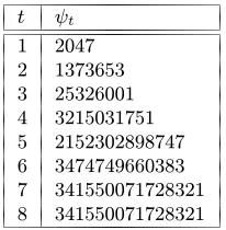
4.29 Definition Letp1, p2, . . . , ptdenote the firsttprimes. Thenψtis defined to be the small-est positive composite integer which is a strong pseudoprime to all the basesp1, p2, . . . , pt.
The numbersψtcan be interpreted as follows: to determine the primality of any integer
n < ψt, it is sufficient to apply the Miller-Rabin algorithm tonwith the basesabeing the firsttprime numbers. With this choice of bases, the answer returned by Miller-Rabin is always correct. Table 4.1 gives the value ofψtfor1≤t≤8.
t ψt
1 2047 2 1373653 3 25326001 4 3215031751 5 2152302898747 6 3474749660383 7 341550071728321 8 341550071728321
Table 4.1:Smallest strong pseudoprimes. The table lists values ofψt, the smallest positive composite
integer that is a strong pseudoprime to each of the firsttprime bases, for1≤t≤8.
4.2.4 Comparison: Fermat, Solovay-Strassen, and Miller-Rabin
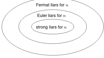
Fact 4.30 describes the relationships between Fermat liars, Euler liars, and strong liars (see Definitions 4.7, 4.15, and 4.21).
4.30 Fact Letnbe an odd composite integer.
§4.2 Probabilistic primality tests 141
4.31 Example (Fermat, Euler, strong liars) Consider the composite integern = 65(= 5× 13). The Fermat liars for65are{1,8,12,14,18,21,27,31,34,38,44,47,51,53,57,64}. The Euler liars for65are {1,8,14,18,47,51,57,64}, while the strong liars for65 are
{1,8,18,47,57,64}.
For a fixed composite candidaten, the situation is depicted in Figure 4.1. This
set-strong liars forn
Fermat liars forn
Euler liars forn
Figure 4.1:Relationships between Fermat, Euler, and strong liars for a composite integern.
tles the question of the relative accuracy of the Fermat, Solovay-Strassen, and Miller-Rabin tests, not only in the sense of the relative correctness of each test on a fixed candidaten, but also in the sense that givenn, the specified containments hold foreachrandomly chosen basea. Thus, from a correctness point of view, the Miller-Rabin test is never worse than the Solovay-Strassen test, which in turn is never worse than the Fermat test. As the following result shows, there are, however, some composite integersnfor which the Solovay-Strassen and Miller-Rabin tests are equally good.
4.32 Fact Ifn≡3 (mod 4), thenais an Euler liar fornif and only if it is a strong liar forn.
What remains is a comparison of the computational costs. While the Miller-Rabin test may appear more complex, it actually requires, at worst, the same amount of computation as Fermat’s test in terms of modular multiplications; thus the Miller-Rabin test is better than Fermat’s test in all regards. At worst, the sequence of computations defined in MILLER-RABIN(n,1) requires the equivalent of computinga(n−1)/2modn. It is also the case that
MILLER-RABIN(n,1) requires less computation than SOLOVAY-STRASSEN(n,1), the latter requiring the computation ofa(n−1)/2modnand possibly a further Jacobi symbol
computation. For this reason, the Solovay-Strassen test is both computationally and con-ceptually more complex.
4.33 Note (Miller-Rabin is better than Solovay-Strassen) In summary, both the Miller-Rabin and Solovay-Strassen tests are correct in the event that either their input is actually prime, or that they declare their input composite. There is, however, no reason to use the Solovay-Strassen test (nor the Fermat test) over the Miller-Rabin test. The reasons for this are sum-marized below.
(i) The Solovay-Strassen test is computationally more expensive.
(ii) The Solovay-Strassen test is harder to implement since it also involves Jacobi symbol computations.
(iv) Any strong liar fornis also an Euler liar forn. Hence, from a correctness point of view, the Miller-Rabin test is never worse than the Solovay-Strassen test.
4.3 (True) Primality tests
The primality tests in this section are methods by which positive integers can beproven
to be prime, and are often referred to asprimality proving algorithms. These primality tests are generally more computationally intensive than the probabilistic primality tests of §4.2. Consequently, before applying one of these tests to a candidate primen, the candidate should be subjected to a probabilistic primality test such as Miller-Rabin (Algorithm 4.24).
4.34 Definition An integernwhich is determined to be prime on the basis of a primality prov-ing algorithm is called aprovable prime.
4.3.1 Testing Mersenne numbers
Efficient algorithms are known for testing primality of some special classes of numbers, such as Mersenne numbers and Fermat numbers. Mersenne primesnare useful because the arithmetic in the fieldZnfor suchncan be implemented very efficiently (see§14.3.4). The Lucas-Lehmer test for Mersenne numbers (Algorithm 4.37) is such an algorithm.
4.35 Definition Lets≥2be an integer. AMersenne numberis an integer of the form2s−1. If2s−1is prime, then it is called aMersenne prime.
The following are necessary and sufficient conditions for a Mersenne number to be prime.
4.36 Fact Lets≥3. The Mersenne numbern= 2s−1is prime if and only if the following two conditions are satisfied:
(i) sis prime; and
(ii) the sequence of integers defined byu0 = 4anduk+1= (u2k−2) modnfork≥0 satisfiesus−2= 0.
Fact 4.36 leads to the following deterministic polynomial-time algorithm for determin-ing (with certainty) whether a Mersenne number is prime.
4.37 AlgorithmLucas-Lehmer primality test for Mersenne numbers
INPUT: a Mersenne numbern= 2s−1withs≥3.
OUTPUT: an answer “prime” or “composite” to the question: “Isnprime?”
1. Use trial division to check ifshas any factors between2and⌊√s⌋. If it does, then return(“composite”).
2. Setu←4.
3. Forkfrom 1 tos−2do the following: computeu←(u2−2) modn.
4. Ifu= 0then return(“prime”). Otherwise, return(“composite”).
§4.3 (True) Primality tests 143
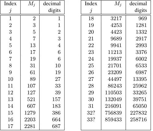
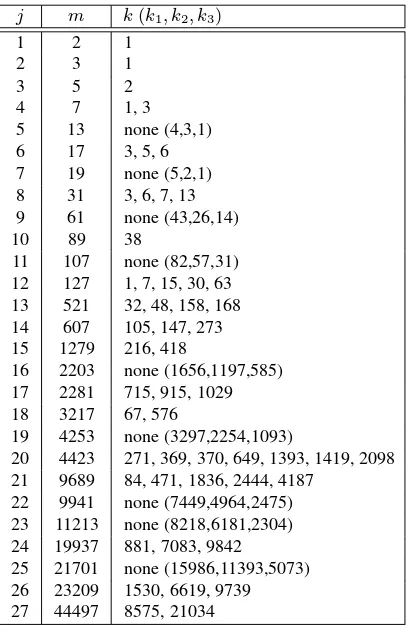
Table 4.2:Known Mersenne primes. The table shows the33known exponentsMj,1≤j≤33, for
which2Mj−1is a Mersenne prime, and also the number of decimal digits in2Mj−1. The question
marks afterj= 32andj= 33indicate that it is not known whether there are any other exponentss
betweenM31and these numbers for which2s−1is prime.
4.3.2 Primality testing using the factorization of
n
−
1
This section presents results which can be used to prove that an integernis prime, provided that the factorization or a partial factorization ofn−1is known. It may seem odd to consider a technique which requires the factorization ofn−1as a subproblem — if integers of this size can be factored, the primality ofnitself could be determined by factoringn. However, the factorization ofn−1may be easier to compute ifnhas a special form, such as aFermat numbern = 22k
+ 1. Another situation where the factorization ofn−1may be easy to compute is when the candidatenis “constructed” by specific methods (see§4.4.4).
4.38 Fact Letn ≥ 3be an integer. Thennis prime if and only if there exists an integera
satisfying:
(i) an−1≡1 (mod n); and
(ii) a(n−1)/q ≡1 (modn)for each prime divisorqofn−1.
This result follows from the fact thatZ∗nhas an element of ordern−1(Definition 2.128) if and only ifnis prime; an elementasatisfying conditions (i) and (ii) has ordern−1.
4.39 Note (primality test based on Fact 4.38) Ifnis a prime, the number of elements of order
n≥ 5(Fact 2.102). Thus, if such anais not found after a “reasonable” number (for ex-ample,12 ln lnn) of iterations, thennis probably composite and should again be subjected to a probabilistic primality test such as Miller-Rabin (Algorithm 4.24).3This method is, in effect, a probabilistic compositeness test.
The next result gives a method for proving primality which requires knowledge of only apartialfactorization ofn−1.
4.40 Fact (Pocklington’s theorem) Letn≥3be an integer, and letn=RF+ 1(i.e.Fdivides
n−1) where the prime factorization ofF isF = t j=1q
ej
j . If there exists an integera satisfying:
(i) an−1≡1 (mod n); and
(ii) gcd(a(n−1)/qj−1, n) = 1for eachj,1≤j≤t,
then every prime divisorpofnis congruent to 1 moduloF. It follows that ifF >√n−1, thennis prime.
Ifnis indeed prime, then the following result establishes that most integersasatisfy conditions (i) and (ii) of Fact 4.40, provided that the prime divisors ofF > √n−1are sufficiently large.
4.41 Fact Letn=RF + 1be an odd prime withF > √n−1andgcd(R, F) = 1. Let the distinct prime factors ofFbeq1,q2, . . . , qt. Then the probability that a randomly selected basea,1≤a ≤n−1, satisfies both: (i)an−1 ≡1 (modn); and (ii)gcd(a(n−1)/qj −
1, n) = 1for eachj,1≤j ≤t, ist
j=1(1−1/qj)≥1−
t j=11/qj.
Thus, if the factorization of a divisorF >√n−1ofn−1is known then to testnfor primality, one may simply choose random integersain the interval[2, n−2]until one is found satisfying conditions (i) and (ii) of Fact 4.40, implying thatnis prime. If such ana
is not found after a “reasonable” number of iterations,4thennis probably composite and this could be established by subjecting it to a probabilistic primality test (footnote 3 also applies here). This method is, in effect, a probabilistic compositeness test.
The next result gives a method for proving primality which only requires the factoriza-tion of a divisorFofn−1that is greater than√3
n. For an example of the use of Fact 4.42, see Note 4.63.
4.42 Fact Letn ≥ 3be an odd integer. Letn = 2RF + 1, and suppose that there exists an integerasatisfying both: (i)an−1 ≡ 1 (modn); and (ii)gcd(a(n−1)/q−1, n) = 1for each prime divisorqofF. Letx≥0andybe defined by2R=xF +yand0≤y < F. IfF ≥√3
nand ify2−4xis neither0nor a perfect square, thennis prime.
4.3.3 Jacobi sum test
TheJacobi sum test is another true primality test. The basic idea is to test a set of con-gruences which are analogues of Fermat’s theorem (Fact 2.127(i)) in certaincyclotomic rings. The running time of the Jacobi sum test for determining the primality of an integer
nisO((lnn)cln ln lnn)bit operations for some constantc. This is “almost” a polynomial-time algorithm since the exponentln ln lnnacts like a constant for the range of values for
3Another approach is to run both algorithms in parallel (with an unlimited number of iterations), until one of
them stops with a definite conclusion “prime” or “composite”.
4The number of iterations may be taken to beTwherePT≤(1
2)100, and whereP = 1−
t
§4.4 Prime number generation 145
nof interest. For example, ifn ≤ 2512, thenln ln lnn < 1.78. The version of the
Ja-cobi sum primality test used in practice is a randomized algorithm which terminates within
O(k(lnn)cln ln lnn)steps with probability at least1−(1
2)k for everyk ≥1, and always
gives a correct answer. One drawback of the algorithm is that it does not produce a “certifi-cate” which would enable the answer to be verified in much shorter time than running the algorithm itself.
The Jacobi sum test is, indeed, practical in the sense that the primality of numbers that are several hundred decimal digits long can be handled in just a few minutes on a com-puter. However, the test is not as easy to program as the probabilistic Miller-Rabin test (Algorithm 4.24), and the resulting code is not as compact. The details of the algorithm are complicated and are not given here; pointers to the literature are given in the chapter notes on page 166.
4.3.4 Tests using elliptic curves
Elliptic curve primality proving algorithms are based on an elliptic curve analogue of Pock-lington’s theorem (Fact 4.40). The version of the algorithm used in practice is usually re-ferred to asAtkin’s testor theElliptic Curve Primality Proving algorithm(ECPP). Under heuristic arguments, the expected running time of this algorithm for proving the primality of an integernhas been shown to beO((lnn)6+ǫ)bit operations for anyǫ >0. Atkin’s test has the advantage over the Jacobi sum test (§4.3.3) that it produces a shortcertificate of primalitywhich can be used to efficiently verify the primality of the number. Atkin’s test has been used to prove the primality of numbers more than 1000 decimal digits long.
The details of the algorithm are complicated and are not presented here; pointers to the literature are given in the chapter notes on page 166.
4.4 Prime number generation
This section considers algorithms for the generation of prime numbers for cryptographic purposes. Four algorithms are presented: Algorithm 4.44 for generatingprobableprimes (see Definition 4.5), Algorithm 4.53 for generatingstrongprimes (see Definition 4.52), Al-gorithm 4.56 for generatingprobableprimespandqsuitable for use in the Digital Signature Algorithm (DSA), and Algorithm 4.62 for generatingprovableprimes (see Definition 4.34).
4.43 Note (prime generation vs. primality testing) Prime numbergenerationdiffers from pri-malitytestingas described in§4.2 and§4.3, but may and typically does involve the latter. The former allows the construction of candidates of a fixed form which may lead to more efficient testing than possible for random candidates.
4.4.1 Random search for probable primes
by MILLER-RABIN(n,t) (Algorithm 4.24) for an appropriate value of the security param-etert(discussed below).
If a randomk-bit odd integernis divisible by a small prime, it is less computationally expensive to rule out the candidatenby trial division than by using the Miller-Rabin test. Since the probability that a random integernhas a small prime divisor is relatively large, before applying the Miller-Rabin test, the candidatenshould be tested for small divisors below a pre-determined boundB. This can be done by dividingnby all the primes below
B, or by computing greatest common divisors ofnand (pre-computed) products of several of the primes≤ B. The proportion of candidate odd integersnnot ruled out by this trial division is
3≤p≤B(1−1p)which, by Mertens’s theorem, is approximately1.12/lnB(here
pranges over prime values). For example, ifB = 256, then only 20% of candidate odd integersnpass the trial division stage, i.e., 80% are discarded before the more costly Miller-Rabin test is performed.
4.44 AlgorithmRandom search for a prime using the Miller-Rabin test
RANDOM-SEARCH(k,t)
INPUT: an integerk, and a security parametert(cf. Note 4.49). OUTPUT: a randomk-bit probable prime.
1. Generate an oddk-bit integernat random.
2. Use trial division to determine whethernis divisible by any odd prime≤ B (see Note 4.45 for guidance on selectingB). If it is then go to step 1.
3. If MILLER-RABIN(n,t) (Algorithm 4.24) outputs “prime” then return(n). Otherwise, go to step 1.
4.45 Note (optimal trial division boundB) LetEdenote the time for a fullk-bit modular ex-ponentiation, and letDdenote the time required for ruling out one small prime as divisor of ak-bit integer. (The valuesEandDdepend on the particular implementation of long-integer arithmetic.) Then the trial division boundBthat minimizes the expected running time of Algorithm 4.44 for generating ak-bit prime is roughlyB =E/D. A more accurate estimate of the optimum choice forBcan be obtained experimentally. The odd primes up toBcan be precomputed and stored in a table. If memory is scarce, a value ofB that is smaller than the optimum value may be used.
Since the Miller-Rabin test does not provide a mathematical proof that a number is in-deed prime, the numbernreturned by Algorithm 4.44 is a probable prime (Definition 4.5). It is important, therefore, to have an estimate of the probability thatnis in fact composite.
4.46 Definition The probability that RANDOM-SEARCH(k,t) (Algorithm 4.44) returns a composite number is denoted bypk,t.
4.47 Note (remarks on estimatingpk,t) It is tempting to conclude directly from Fact 4.25 that
pk,t≤(14)t. This reasoning is flawed (although typically the conclusion will be correct in practice) since it does not take into account the distribution of the primes. (For example, if all candidatesnwere chosen from a setSof composite numbers, the probability of error is 1.) The following discussion elaborates on this point. LetX represent the event thatnis composite, and letYtdenote the event than MILLER-RABIN(n,t) declaresnto be prime. Then Fact 4.25 states thatP(Yt|X)≤(14)t. What is relevant, however, to the estimation of
§4.4 Prime number generation 147
from a setSof odd numbers, and supposepis the probability thatnis prime (this depends on the candidate setS). Assume also that0< p <1. Then by Bayes’ theorem (Fact 2.10):
P(X|Yt) = P(X)P(Yt|X) small. However, the error-probability of Miller-Rabin is usually far smaller than(1
4)t(see
Remark 4.26). Using better estimates forP(Yt|X)and estimates on the number ofk-bit prime numbers, it has been shown thatpk,tis, in fact, smaller than(14)tfor all sufficiently largek. A more concrete result is the following: if candidatesnare chosen at random from the set of odd numbers in the interval[3, x], thenP(X|Yt)≤(14)tfor allx≥1060.
Further refinements forP(Yt|X)allow the following explicit upper bounds onpk,tfor various values ofkandt.5
4.48 Fact (some upper bounds onpk,tin Algorithm 4.44)
(i) pk,1< k242−
words, the probability that RANDOM-SEARCH(512,6) returns a 512-bit composite integer is less than(1
2)88. Using more advanced techniques, the upper bounds onpk,tgiven by
Fact 4.48 have been improved. These upper bounds arise from complicated formulae which are not given here. Table 4.3 lists some improved upper bounds onpk,tfor some sample values ofkandt. As an example, the probability that RANDOM-SEARCH(500,6) returns a composite number is≤ (1
Table 4.3:Upper bounds onpk,tfor sample values ofkandt. An entryjcorresponding tokandt
impliespk,t≤(12)j.
5The estimates ofp
k,tpresented in the remainder of this subsection were derived for the situation where
Al-gorithm 4.44 does not use trial division by small primes to rule out some candidatesn. Since trial division never rules out a prime, it can only give a better chance of rejecting composites. Thus the error probabilitypk,tmight
4.49 Note (controlling the error probability) In practice, one is usually willing to tolerate an er-ror probability of(1
2)80when using Algorithm 4.44 to generate probable primes. For
sam-ple values ofk, Table 4.4 lists the smallest value oftthat can be derived from Fact 4.48 for whichpk,t≤(12)80. For example, when generating 1000-bit probable primes,
Miller-Rabin witht = 3repetitions suffices. Algorithm 4.44 rules out most candidatesneither by trial division (in step 2) or by performing just one iteration of the Miller-Rabin test (in step 3). For this reason, the only effect of selecting a larger security parameterton the run-ning time of the algorithm will likely be to increase the time required in the final stage when the (probable) prime is chosen.
4.50 Remark (Miller-Rabin test with basea = 2) The Miller-Rabin test involves exponenti-ating the basea; this may be performed using the repeated square-and-multiply algorithm (Algorithm 2.143). Ifa= 2, then multiplication byais a simple procedure relative to mul-tiplying byain general. One optimization of Algorithm 4.44 is, therefore, to fix the base
a= 2when first performing the Miller-Rabin test in step 3. Since most composite numbers will fail the Miller-Rabin test with basea = 2, this modification will lower the expected running time of Algorithm 4.44.
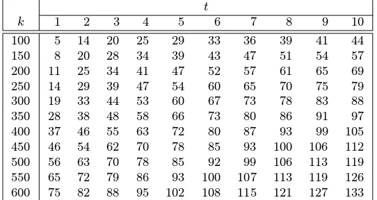
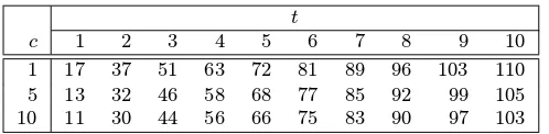
4.51 Note (incremental search)
(i) An alternative technique to generating candidates nat random in step 1 of Algo-rithm 4.44 is to first select a randomk-bit odd numbern0, and then test thesnumbers n=n0, n0+ 2, n0+ 4, . . . , n0+ 2(s−1)for primality. If all thesescandidates are
found to be composite, the algorithm is said to havefailed. Ifs=c·ln 2kwherecis a constant, the probabilityqk,t,sthat this incremental search variant of Algorithm 4.44 returns a composite number has been shown to be less thanδk32−√kfor some con-stantδ. Table 4.5 gives some explicit bounds on this error probability fork= 500and
t≤10. Under reasonable number-theoretic assumptions, the probability of the algo-rithm failing has been shown to be less than2e−2cfor largek(here,e≈2.71828). (ii) Incremental search has the advantage that fewer random bits are required.
Further-more, the trial division by small primes in step 2 of Algorithm 4.44 can be accom-plished very efficiently as follows. First the valuesR[p] = n0modpare computed
for each odd primep≤B. Each time2is added to the current candidate, the values in the tableRare updated asR[p]←(R[p] + 2) modp. The candidate passes the trial division stage if and only if none of theR[p]values equal0.
(iii) IfBis large, an alternative method for doing the trial division is to initialize a table
S[i]←0for0≤ i ≤ (s−1); the entryS[i]corresponds to the candidaten0+ 2i.
§4.4 Prime number generation 149
t
c 1 2 3 4 5 6 7 8 9 10
1 17 37 51 63 72 81 89 96 103 110 5 13 32 46 58 68 77 85 92 99 105 10 11 30 44 56 66 75 83 90 97 103
Table 4.5:Upper bounds on the error probability of incremental search (Note 4.51) fork = 500 and sample values ofcandt. An entryjcorresponding tocandtimpliesq500,t,s ≤(12)j, where
s=c·ln 2500.
which(n0+ 2j)≡0 (modp). ThenS[j]and eachpthentry after it are set to1. A
candidaten0+ 2ithen passes the trial division stage if and only ifS[i] = 0. Note
that the estimate for the optimal trial division boundBgiven in Note 4.45 does not apply here (nor in (ii)) since the cost of division is amortized over all candidates.
4.4.2 Strong primes
The RSA cryptosystem (§8.2) uses a modulus of the formn=pq, wherepandqare dis-tinct odd primes. The primespandqmust be of sufficient size that factorization of their product is beyond computational reach. Moreover, they should be random primes in the sense that they be chosen as a function of a random input through a process defining a pool of candidates of sufficient cardinality that an exhaustive attack is infeasible. In practice, the resulting primes must also be of a pre-determined bitlength, to meet system specifications. The discovery of the RSA cryptosystem led to the consideration of several additional con-straints on the choice ofpandqwhich are necessary to ensure the resulting RSA system safe from cryptanalytic attack, and the notion of a strong prime (Definition 4.52) was defined. These attacks are described at length in Note 8.8(iii); as noted there, it is now believed that strong primes offer little protection beyond that offered by random primes, since randomly selected primes of the sizes typically used in RSA moduli today will satisfy the constraints with high probability. On the other hand, they are no less secure, and require only minimal additional running time to compute; thus, there is little real additional cost in using them.
4.52 Definition A prime numberpis said to be astrong primeif integersr,s, andtexist such that the following three conditions are satisfied:
(i) p−1has a large prime factor, denotedr; (ii) p+ 1has a large prime factor, denoteds; and (iii) r−1has a large prime factor, denotedt.
4.53 AlgorithmGordon’s algorithm for generating a strong prime
SUMMARY: a strong primepis generated.
1. Generate two large random primessandtof roughly equal bitlength (see Note 4.54). 2. Select an integeri0. Find the first prime in the sequence2it+ 1, fori = i0, i0+
1, i0+ 2, . . . (see Note 4.54). Denote this prime byr= 2it+ 1.
3. Computep0= 2(sr−2modr)s−1.
4. Select an integerj0. Find the first prime in the sequencep0+ 2jrs, forj =j0, j0+
1, j0+ 2, . . . (see Note 4.54). Denote this prime byp=p0+ 2jrs.
5. Return(p).
Justification. To see that the primepreturned by Gordon’s algorithm is indeed a strong prime, observe first (assumingr=s) thatsr−1≡1 (modr); this follows from Fermat’s
theorem (Fact 2.127). Hence,p0≡1 (modr)andp0≡ −1 (mods). Finally (cf.
Defi-nition 4.52),
(i) p−1 =p0+ 2jrs−1≡0 (mod r), and hencep−1has the prime factorr;
(ii) p+ 1 =p0+ 2jrs+ 1≡0 (mod s), and hencep+ 1has the prime factors; and
(iii) r−1 = 2it≡0 (modt), and hencer−1has the prime factort.
4.54 Note (implementing Gordon’s algorithm)
(i) The primessandtrequired in step 1 can be probable primes generated by Algo-rithm 4.44. The Miller-Rabin test (AlgoAlgo-rithm 4.24) can be used to test each candidate for primality in steps 2 and 4, after ruling out candidates that are divisible by a small prime less than some boundB. See Note 4.45 for guidance on selectingB. Since the Miller-Rabin test is a probabilistic primality test, the output of this implementation of Gordon’s algorithm is a probable prime.
(ii) By carefully choosing the sizes of primess,tand parametersi0,j0, one can control
the exact bitlength of the resulting primep. Note that the bitlengths ofrandswill be about half that ofp, while the bitlength oftwill be slightly less than that ofr.
4.55 Fact (running time of Gordon’s algorithm) If the Miller-Rabin test is the primality test used in steps 1, 2, and 4, the expected time Gordon’s algorithm takes to find a strong prime is only about 19% more than the expected time Algorithm 4.44 takes to find a random prime.
4.4.3 NIST method for generating DSA primes
Some public-key schemes require primes satisfying various specific conditions. For exam-ple, the NIST Digital Signature Algorithm (DSA of§11.5.1) requires two primespandq
satisfying the following three conditions:
(i) 2159< q <2160; that is,qis a160-bit prime;
(ii) 2L−1< p <2Lfor a specifiedL, whereL= 512 + 64lfor some0≤l≤8; and (iii) qdividesp−1.
This section presents an algorithm for generating such primespandq. In the following,
H denotes the SHA-1 hash function (Algorithm 9.53) which maps bitstrings of bitlength
<264to160-bit hash-codes. Where required, an integerxin the range0≤x <2gwhose binary representation isx=xg−12g−1+xg−22g−2+· · ·+x222+x12 +x0should be
§4.4 Prime number generation 151
4.56 AlgorithmNIST method for generating DSA primes
INPUT: an integerl,0≤l≤8.
OUTPUT: a160-bit primeqand anL-bit primep, whereL= 512 + 64landq|(p−1). 1. ComputeL= 512 + 64l. Using long division of(L−1)by160, findn,bsuch that
L−1 = 160n+b, where0≤b <160. 2. Repeat the following:
2.1 Choose a random seeds(not necessarily secret) of bitlengthg≥160. 2.2 ComputeU =H(s)⊕H((s+ 1) mod 2g).
2.3 FormqfromU by setting to1the most significant and least significant bits of
U. (Note thatqis a160-bit odd integer.)
2.4 Testqfor primality using MILLER-RABIN(q,t) fort≥18(see Note 4.57). Untilqis found to be a (probable) prime.
3. Seti←0,j←2.
4. Whilei <4096do the following:
4.1 Forkfrom0tondo the following: setVk←H((s+j+k) mod 2g). 4.2 For the integerW defined below, letX =W+ 2L−1. (Xis anL-bit integer.)
W =V0+V12160+V22320+· · ·+Vn−12160(n−1)+ (Vnmod 2b)2160n.
4.3 Computec=X mod 2qand setp=X−(c−1). (Note thatp≡1 (mod 2q).) 4.4 Ifp≥2L−1then do the following:
Testpfor primality using MILLER-RABIN(p,t) fort≥5(see Note 4.57). Ifpis a (probable) prime then return(q,p).
4.5 Seti←i+ 1,j←j+n+ 1. 5. Go to step 2.
4.57 Note (choice of primality test in Algorithm 4.56)
(i) The FIPS 186 document where Algorithm 4.56 was originally described only speci-fies that arobustprimality test be used in steps 2.4 and 4.4, i.e., a primality test where the probability of a composite integer being declared prime is at most(12)80. If the
heuristic assumption is made thatqis a randomly chosen160-bit integer then, by Ta-ble 4.4, MILLER-RABIN(q,18) is a robust test for the primality ofq. Ifpis assumed to be a randomly chosenL-bit integer, then by Table 4.4, MILLER-RABIN(p,5) is a robust test for the primality ofp. Since the Miller-Rabin test is a probabilistic pri-mality test, the output of Algorithm 4.56 is a probable prime.
(ii) To improve performance, candidate primesqandpshould be subjected to trial divi-sion by all odd primes less than some boundBbefore invoking the Miller-Rabin test. See Note 4.45 for guidance on selectingB.
4.4.4 Constructive techniques for provable primes
Maurer’s algorithm (Algorithm 4.62) generates randomprovableprimes that are almost uniformly distributed over the set of all primes of a specified size. The expected time for generating a prime is only slightly greater than that for generating a probable prime of equal size using Algorithm 4.44 with security parametert = 1. (In practice, one may wish to chooset >1in Algorithm 4.44; cf. Note 4.49.)
The main idea behind Algorithm 4.62 is Fact 4.59, which is a slight modification of Pocklington’s theorem (Fact 4.40) and Fact 4.41.
4.59 Fact Letn≥3be an odd integer, and suppose thatn= 1 + 2Rqwhereqis an odd prime. Suppose further thatq > R.
(i) If there exists an integerasatisfyingan−1≡1 (modn)andgcd(a2R−1, n) = 1, thennis prime.
(ii) Ifnis prime, the probability that a randomly selected basea,1≤a≤n−1, satisfies
an−1≡1 (mod n)andgcd(a2R−1, n) = 1is(1−1/q).
Algorithm 4.62 recursively generates an odd primeq, and then chooses random integersR,
R < q, untiln = 2Rq+ 1can be proven prime using Fact 4.59(i) for some basea. By Fact 4.59(ii) the proportion of such bases is1−1/qfor primen. On the other hand, ifnis composite, then most basesawill fail to satisfy the conditionan−1≡1 (modn).
4.60 Note (description of constantscandmin Algorithm 4.62)
(i) The optimal value of the constantc defining the trial division boundB = ck2 in
step 2 depends on the implementation of long-integer arithmetic, and is best deter-mined experimentally (cf. Note 4.45).
(ii) The constantm = 20ensures thatIis at least20bits long and hence the interval from whichRis selected, namely[I+ 1,2I], is sufficiently large (for the values of
kof practical interest) that it most likely contains at least one valueRfor whichn= 2Rq+ 1is prime.
4.61 Note (relative sizerofqwith respect tonin Algorithm 4.62) Therelative sizerofqwith respect tonis defined to ber= lgq/lgn. In order to assure that the generated primenis chosen randomly with essentially uniform distribution from the set of allk-bit primes, the size of the prime factorqofn−1must be chosen according to the probability distribution of the largest prime factor of a randomly selectedk-bit integer. Sinceqmust be greater than
Rin order for Fact 4.59 to apply, the relative sizerofqis restricted to being in the interval [12,1]. It can be deduced from Fact 3.7(i) that the cumulative probability distribution of the relative sizerof the largest prime factor of a large random integer, given thatris at least
1
2, is(1 + lgr)for 12 ≤r≤1. In step 4 of Algorithm 4.62, the relative sizeris generated
according to this distribution by selecting a random numbers∈[0,1]and then settingr= 2s−1. Ifk≤2mthenris chosen to be the smallest permissible value, namely 1
2, in order
§4.4 Prime number generation 153
4.62 AlgorithmMaurer’s algorithm for generating provable primes
PROVABLE PRIME(k) INPUT: a positive integerk. OUTPUT: ak-bit prime numbern.
1. (Ifkis small, then test random integers by trial division. A table of small primes may be precomputed for this purpose.)
Ifk≤20then repeatedly do the following: 1.1 Select a randomk-bit odd integern.
1.2 Use trial division by all primes less than√nto determine whethernis prime. 1.3 Ifnis prime then return(n).
2. Setc←0.1andm←20(see Note 4.60).
3. (Trial division bound) SetB←c·k2(see Note 4.60).
4. (Generater, the size ofqrelative ton— see Note 4.61) Ifk >2mthen repeatedly do the following: select a random numbersin the interval[0,1], setr←2s−1, until
(k−rk)> m. Otherwise (i.e.k≤2m), setr←0.5. 5. Computeq←PROVABLE PRIME(⌊r·k⌋+ 1). 6. SetI←⌊2k−1/(2q)⌋.
7. success←0.
8. While (success= 0) do the following:
8.1 (select a candidate integern) Select a random integerRin the interval[I+ 1,2I]and setn←2Rq+ 1.
8.2 Use trial division to determine whethernis divisible by any prime number< B. If it is not then do the following:
Select a random integerain the interval[2, n−2]. Computeb←an−1modn.
Ifb= 1then do the following:
Computeb←a2Rmodnandd←gcd(b−1, n). Ifd= 1then success←1.
9. Return(n).
4.63 Note (improvements to Algorithm 4.62)
(i) A speedup can be achieved by using Fact 4.42 instead of Fact 4.59(i) for proving
n= 2Rq+ 1prime in step 8.2 of Maurer’s algorithm — Fact 4.42 only requires that
qbe greater than√3 n.
(ii) If a candidatenpasses the trial division (in step 8.2), then a Miller-Rabin test (Algo-rithm 4.24) with the single basea = 2should be performed onn; only ifnpasses this test should the attempt to prove its primality (the remainder of step 8.2) be under-taken. This leads to a faster implementation due to the efficiency of the Miller-Rabin test with a single basea= 2(cf. Remark 4.50).
(iii) Step 4 requires the use of real number arithmetic when computing2s−1. To avoid
these computations, one can precompute and store a list of such values for a selection of random numberss∈[0,1].
to its recursive nature. Provable primes are preferable to probable primes in the sense that the former have zero error probability. In any cryptographic application, however, there is always a non-zero error probability of some catastrophic failure, such as the adversary guessing a secret key or hardware failure. Since the error probability of probable primes can be efficiently brought down to acceptably low levels (see Note 4.49 but note the depen-dence ont), there appears to be no reason for mandating the use of provable primes over probable primes.
4.5 Irreducible polynomials over
Z
pRecall (Definition 2.190) that a polynomialf(x) ∈ Zp[x]of degreem ≥ 1is said to be
irreducible overZpif it cannot be written as a product of two polynomials inZp[x]each having degree less thanm. Such a polynomialf(x)can be used to represent the elements of the finite fieldFpm asFpm = Zp[x]/(f(x)), the set of all polynomials inZp[x]of
de-gree less thanmwhere the addition and multiplication of polynomials is performed modulo
f(x)(see§2.6.3). This section presents techniques for constructing irreducible polynomials overZp, wherepis a prime. The characteristic two finite fieldsF2mare of particular
inter-est for cryptographic applications because the arithmetic in these fields can be efficiently performed both in software and in hardware. For this reason, additional attention is given to the special case of irreducible polynomials overZ2.
The arithmetic in finite fields can usually be implemented more efficiently if the irre-ducible polynomial chosen has few non-zero terms. Irreirre-ducibletrinomials, i.e., irreducible polynomials having exactly three non-zero terms, are considered in§4.5.2.Primitive poly-nomials, i.e., irreducible polynomialsf(x)of degreeminZp[x]for whichxis a generator ofF∗pm, the multiplicative group of the finite fieldFpm=Zp[x]/(f(x))(Definition 2.228),
are the topic of§4.5.3. Primitive polynomials are also used in the generation of linear feed-back shift register sequences having the maximum possible period (Fact 6.12).
4.5.1 Irreducible polynomials
Iff(x)∈Zp[x]is irreducible overZpandais a non-zero element inZp, thena·f(x)is also irreducible overZp. Hence it suffices to restrict attention tomonicpolynomials inZp[x], i.e., polynomials whose leading coefficient is 1. Observe also that iff(x)is an irreducible polynomial, then its constant term must be non-zero. In particular, iff(x) ∈Z2[x], then
its constant term must be 1.
There is a formula for computing exactly the number of monic irreducible polynomi-als inZp[x]of a fixed degree. The M¨obius function, which is defined next, is used in this formula.
4.65 Definition Letmbe a positive integer. TheM¨obius functionµis defined by
µ(m) =
1, ifm= 1,
0, ifmis divisible by the square of a prime,
(−1)k, ifmis the product ofkdistinct primes.
4.66 Example (M¨obius function) The following table gives the values of the M¨obius function
§4.5 Irreducible polynomials overZp 155
m 1 2 3 4 5 6 7 8 9 10
µ(m) 1 −1 −1 0 −1 1 −1 0 0 1
4.67 Fact (number of monic irreducible polynomials) Letpbe a prime andma positive integer. (i) The numberNp(m)of monic irreducible polynomials of degreeminZp[x]is given
by the following formula:
Np(m) = 1
m
d|m
µ(d)pm/d,
where the summation ranges over all positive divisorsdofm.
(ii) The probability of a random monic polynomial of degreeminZp[x]being irreducible overZpis roughly m1. More specifically, the numberNp(m)satisfies
1 2m ≤
Np(m)
pm ≈
1
m.
Testing irreducibility of polynomials inZp[x]is significantly simpler than testing pri-mality of integers. A polynomial can be tested for irreducibility by verifying that it has no irreducible factors of degree≤ ⌊m2⌋. The following result leads to an efficient method (Al-gorithm 4.69) for accomplishing this.
4.68 Fact Letpbe a prime and letkbe a positive integer.
(i) The product of all monic irreducible polynomials inZp[x]of degree dividingkis equal toxpk
−x.
(ii) Letf(x)be a polynomial of degreeminZp[x]. Thenf(x)is irreducible overZpif and only ifgcd(f(x), xpi
−x) = 1for eachi,1≤i≤ ⌊m
2⌋.
4.69 AlgorithmTesting a polynomial for irreducibility
INPUT: a primepand a monic polynomialf(x)of degreeminZp[x]. OUTPUT: an answer to the question: “Isf(x)irreducible overZp?”
1. Setu(x)←x. 2. Forifrom 1 to⌊m
2⌋do the following:
2.1 Computeu(x)←u(x)pmodf(x)using Algorithm 2.227. (Note thatu(x)is a polynomial inZp[x]of degree less thanm.)
2.2 Computed(x) = gcd(f(x), u(x)−x)(using Algorithm 2.218). 2.3 Ifd(x)= 1then return(“reducible”).
3. Return(“irreducible”).
Fact 4.67 suggests that one method for finding an irreducible polynomial of degreem
4.70 AlgorithmGenerating a random monic irreducible polynomial overZp
INPUT: a primepand a positive integerm.
OUTPUT: a monic irreducible polynomialf(x)of degreeminZp[x]. 1. Repeat the following:
1.1 (Generate a random monic polynomial of degreeminZp[x])
Randomly select integersa0, a1, a2, . . . , am−1between0andp−1witha0=
0. Letf(x)be the polynomialf(x) =xm+am−1xm−1+· · ·+a2x2+a1x+a0.
1.2 Use Algorithm 4.69 to test whetherf(x)is irreducible overZp. Untilf(x)is irreducible.
2. Return(f(x)).
It is known that the expected degree of the irreducible factor of least degree of a random polynomial of degreeminZp[x]isO(lgm). Hence for each choice off(x), the expected number of times steps 2.1 – 2.3 of Algorithm 4.69 are iterated isO(lgm). Each iteration takesO((lgp)m2)Zp-operations. These observations, together with Fact 4.67(ii), deter-mine the running time for Algorithm 4.70.
4.71 Fact Algorithm 4.70 has an expected running time ofO(m3(lgm)(lgp))Z
p-operations.
Given one irreducible polynomial of degreemoverZp, Note 4.74 describes a method, which is more efficient than Algorithm 4.70, for randomly generating additional such poly-nomials.
4.72 Definition LetFqbe a finite field of characteristicp, and letα∈Fq. Aminimum
polyno-mialofαoverZpis a monic polynomial of least degree inZp[x]havingαas a root.
4.73 Fact LetFqbe a finite field of orderq=pm, and letα∈Fq.
(i) The minimum polynomial ofαoverZp, denotedmα(x), is unique. (ii) mα(x)is irreducible overZp.
(iii) The degree ofmα(x)is a divisor ofm.
(iv) Lettbe the smallest positive integer such thatαpt
= α. (Note that such atexists since, by Fact 2.213,αpm
=α.) Then
mα(x) = t−1
i=0
(x−αpi). (4.1)
4.74 Note (generating new irreducible polynomials from a given one) Suppose thatf(y)is a given irreducible polynomial of degreemoverZp. The finite fieldFpmcan then be
repre-sented asFpm =Zp[y]/(f(y)). A random monic irreducible polynomial of degreemover Zpcan be efficiently generated as follows. First generate a random elementα∈Fpm and
then, by repeated exponentiation byp, determine the smallest positive integertfor which
αpt
=α. Ift < m, then generate a new random elementα∈Fpmand repeat; the
probabil-ity thatt < mis known to be at most(lgm)/qm/2. If indeedt=m, then computem
α(x) using the formula (4.1). Thenmα(x)is a random monic irreducible polynomial of degree
§4.5 Irreducible polynomials overZp 157
4.5.2 Irreducible trinomials
If a polynomialf(x)inZ2[x]has an even number of non-zero terms, thenf(1) = 0, whence
(x+ 1)is a factor off(x). Hence, the smallest number of non-zero terms an irreducible polynomial of degree≥2inZ2[x]can have is three. An irreducibletrinomialof degreem
inZ2[x]must be of the formxm+xk+ 1, where1≤k≤m−1. Choosing an irreducible
trinomialf(x) ∈ Z2[x]of degreemto represent the elements of the finite fieldF2m = Z2[x]/(f(x))can lead to a faster implementation of the field arithmetic. The following
facts are sometimes of use when searching for irreducible trinomials.
4.75 Fact Letmbe a positive integer, and letkdenote an integer in the interval[1, m−1]. (i) If the trinomialxm+xk+ 1is irreducible overZ
2then so isxm+xm−k+ 1.
(ii) Ifm≡0 (mod 8), there is no irreducible trinomial of degreeminZ2[x].
(iii) Suppose that eitherm≡3 (mod 8)orm≡5 (mod 8). Then a necessary condition forxm+xk+ 1to be irreducible overZ
2is that eitherkorm−kmust be of the
form2dfor some positive divisordofm.
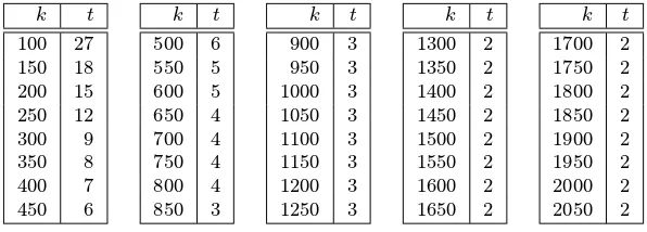
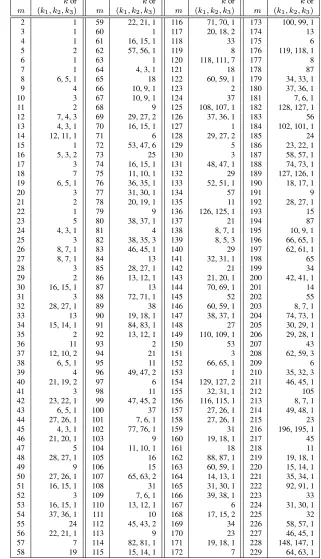
Tables 4.6 and 4.7 list an irreducible trinomial of degreemoverZ2for eachm≤1478
for which such a trinomial exists.
4.5.3 Primitive polynomials
Primitive polynomials were introduced at the beginning of§4.5. Letf(x)∈ Zp[x]be an irreducible polynomial of degreem. If the factorization of the integerpm−1is known, then Fact 4.76 yields an efficient algorithm (Algorithm 4.77) for testing whether or notf(x)is a primitive polynomial. If the factorization ofpm−1is unknown, there is no efficient algorithm known for performing this test.
4.76 Fact Letpbe a prime and let the distinct prime factors ofpm−1ber1, r2, . . . , rt. Then an irreducible polynomialf(x)∈Zp[x]is primitive if and only if for eachi,1≤i≤t:
x(pm−1)/ri
≡1 (modf(x)).
(That is,xis an element of orderpm−1in the fieldZ
p[x]/(f(x)).)
4.77 AlgorithmTesting whether an irreducible polynomial is primitive
INPUT: a primep, a positive integerm, the distinct prime factorsr1, r2, . . . , rtofpm−1, and a monic irreducible polynomialf(x)of degreeminZp[x].
OUTPUT: an answer to the question: “Isf(x)a primitive polynomial?” 1. Forifrom 1 totdo the following:
1.1 Computel(x) =x(pm
−1)/ri modf(x)(using Algorithm 2.227).
1.2 Ifl(x) = 1then return(“not primitive”). 2. Return(“primitive”).