This page
Published by New Age International (P) Ltd., Publishers
All rights reserved.
No part of this ebook may be reproduced in any form, by photostat, microfilm, xerography, or any other means, or incorporated into any information retrieval system, electronic or mechanical, without the written permission of the publisher. All inquiries should be emailed to [email protected]
PUBLISHING FOR ONE WORLD
NEW AGE INTERNATIONAL (P) LIMITED, PUBLISHERS 4835/24, Ansari Road, Daryaganj, New Delhi - 110002
Visit us at www.newagepublishers.com
and mother
and mother
and mother
and mother
This page
It gives me immense pleasure in presenting the first edition of the book-Principles of DATA STRUCTURES Using C and C++ which is a unique text valuable for professionals that covers both theoretical and practical aspects of the data structures.
The study of data structures is an essential subject of every under graduate and graduate programs related to computer science. A thorough understanding of the basics of this subject is inevitable for efficient programming. This book covers all the fundamen-tal topics to give a better understanding about the subject. This book is written in accord-ance with the revised syllabus for BTech/BE (both Computer Science and Electronics branches) and MCA students of Kerala University, MG University, Calicut University, CUSAT Cochin (deemed) University, NIT Calicut (deemed) University, Anna University, UP Techni-cal University, Amritha Viswa (deemed) Vidyapeeth, Karunya (deemed) University, Pune University, Bangalore University and Rajasthan Vidyapeeth (deemed) University. Moreo-ver this book coMoreo-vers almost all the topics of the other Indian and International UniMoreo-versities where this subject is there in their under graduate and graduate programs.
While writing the book, I have always considered the examination requirements of the students and various difficulties and troubles, which they face, while studying the subject.
All effort is made to cover the topics in the simplest possible way without loosing its qualities. Almost five hundred questions from various university question papers have been included in this book. In short, I earnestly hope that the book will earn the apprecia-tion of the teachers and students alike.
Although I have tried to check mistakes and misprints, yet it is difficult to claim perfection. Any suggestions for the improvement of any topics, when brought to my notice, will be thankfully acknowledged and will be incorporated in the next edition.
This page
I praise and give thanks to the Almighty Living Holy God, without His grace nothing is possible for any one.
I take this opportunity to thank everyone, especially my friends and students who have inspired me to write and complete this book. I am indebted to the many published works available on the subject, which have helped me in the prepara-tion of the manuscript.
I express my sincere thanks to Mr. Sreelal, Mr. Rajesh, Mr. Ajith and others for digitalizing the manuscript.
I am also thankful to the following Indian Universities and examination bodies, whose examination papers have been included in the text as self-review ques-tions. Moreover, their syllabus has been kept in view while writing this treatise.
Kerala University Anna University
Calicut University Mahatma Gandhi University
NIT, Calicut CUSAT, Kochi
UP Technical University Amritha Viswa Vidyapeeth Karunya University Rajasthan Vidyapeeth Pune University Bangalore University
This page
Preface ... (vii)
Acknowledgement ... (ix)
1. Programming Methodologies ... 1
1.1. An Introduction to Data Structure ... 1
1.2. Algorithm ... 2
1.3. Stepwise Refinement Techniques ... 2
1.4. Modular Programming ... 3
1.5. Top-Down Algorithm Design ... 3
1.6. Bottom-Up Algorithm Design ... 4
1.7. Structured Programming ... 4
1.8. Analysis of Algorithm ... 5
1.9. Time-Space Trade Off ... 8
1.10. Big “OH” Notation ... 8
1.11. Limitation of Big “OH” Notation ... 9
1.12. Classification of Data Structure ... 9
1.13. Arrays ... 10
1.14. Vectors ... 13
1.15. Lists ... 13
1.16. Files and Records ... 14
1.17. Characteristics of Strings ... 14
Self Review Questions ... 16
2. Memory Management ... 18
2.1. Memory Allocation in C ... 18
2.2. Dynamic Memory Allocation in C++ ... 22
2.3. Free Storage List ... 22
2.4. Garbage Collection ... 23
2.5. Dangling Reference ... 23
2.6. Reference Counters ... 24
2.7. Storage Compaction ... 24
2.8. Boundary Tag Method ... 24
Self Review Questions ... 25
3. The Stack ... 26
3.1. Operations Performed on Stack ... 27
3.2. Stack Implementation ... 27
3.3. Stack Using Arrays ... 27
3.4. Applications of Stacks ... 34
3.5. Converting Infix to Postfix Expression ... 46
3.6. Evaluating Postfix Expression ... 57
4. The Queue ... 65
4.1. Algorithms for Queue Operations ... 67
4.2. Other Queues ... 71
4.3. Circular Queue ... 71
4.4. Deques ... 77
4.5. Applications of Queue ... 86
Self Review Questions ... 86
5. Linked List ... 88
5.1. Linked List ... 88
5.2. Representation of Linked List ... 89
5.3. Advantages and Disadvantages ... 89
5.4. Operation on Linked List ... 90
5.5. Types of Linked List ... 90
5.6. Singly Linked List ... 91
5.7. Stack Using Linked List ... 107
5.8. Queue Using Linked List ... 114
5.9. Queue Using Two Stacks ... 122
5.10. Polynomials Using Linked List ... 126
5.11. Doubly Linked List ... 131
5.12. Circular Linked List ... 140
5.13. Priority Queues ... 146
Self Review Questions ... 151
6. Sorting Techniques ... 153
6.1. Complexity of Sorting Algorithms ... 154
6.2. Bubble Sort ... 154
6.3. Selection Sort ... 159
6.4. Insertion Sort ... 163
6.5. Shell Sort ... 168
6.6. Quick Sort ... 170
6.7. Merge Sort ... 176
6.8. Radix Sort ... 183
6.9. Heap ... 189
6.10. External Sorting ... 200
Self Review Questions ... 205
7. Searching and Hashing ... 207
7.1. Linear or Sequential Searching ... 207
7.2. Binary Search ... 209
7.3. Interpolation Search ... 212
7.5. Hashing ... 219
Self Review Questions ... 227
8. The Trees ... 229
8.1. Basic Terminologies ... 229
8.2. Binary Trees ... 230
8.3. Binary Tree Representation ... 233
8.4. Operations on Binary Tree .. 235
8.5. Traversing Binary Trees Recursively ... 236 8.6. Traversing Binary Tree Non-Recursively ... 246
8.7. Binary Search Trees ... 258
8.8. Threaded Binary Tree ... 272
8.9. Expression Trees ... 273
8.10. Decision Tree ... 275
8.11. Fibanocci Tree ... 275
8.12. Selection Trees ... 277
8.13. Balanced Binary Trees ... 283
8.14. AVL Trees ... 284
8.15. M-Way Search Trees ... 287
8.16. 2-3 Trees ... 287
8.17. 2-3-4 Trees ... 289
8.18. Red-Black Tree ... 290
8.19. B-Tree ... 293
8.20. Splay Trees ... 296
8.21. Digital Search Trees ... 300
8.22. Tries ... 302
Self Review Questions ,.. 303
9. Graphs ... 305
9.1. Basic Terminologies ... 305
9.2. Representation of Graph ... 309
9.3. Operations on Graph ... 313
9.4. Breadth First Search ... 318
9.5. Depth First Search ... 325
9.6. Minimum Spanning Tree ... 327
9.7. Shortest Path ... 347
Self Review Questions ... 355
Bibliography ... 357
This page
Programming Methodologies
Programming methodologies deal with different methods of designing programs. This will teach you how to program efficiently. This book restricts itself to the basics of programming in C and C++, by assuming that you are familiar with the syntax of C and C++ and can write, debug and run programs in C and C++. Discussions in this chapter outline the importance of structuring the programs, not only the data pertaining to the solution of a problem but also the programs that operates on the data.
Data is the basic entity or fact that is used in calculation or manipulation process. There are two types of data such as numerical and alphanumerical data. Integer and floating-point numbers are of numerical data type and strings are of alphanumeric data type. Data may be single or a set of values, and it is to be organized in a particular fashion. This organization or structuring of data will have profound impact on the efficiency of the program.
1.1. AN INTRODUCTION TO DATA STRUCTURE
Data structure is the structural representation of logical relationships between ele-ments of data. In other words a data structure is a way of organizing data items by consid-ering its relationship to each other.
Data structure mainly specifies the structured organization of data, by providing accessing methods with correct degree of associativity. Data structure affects the design of both the structural and functional aspects of a program.
Algorithm + Data Structure = Program
Data structures are the building blocks of a program; here the selection of a particu-lar data structure will help the programmer to design more efficient programs as the complexity and volume of the problems solved by the computer is steadily increasing day by day. The programmers have to strive hard to solve these problems. If the problem is analyzed and divided into sub problems, the task will be much easier i.e., divide, conquer and combine.
A complex problem usually cannot be divided and programmed by set of modules unless its solution is structured or organized. This is because when we divide the big problems into sub problems, these sub problems will be programmed by different pro-grammers or group of propro-grammers. But all the propro-grammers should follow a standard structural method so as to make easy and efficient integration of these modules. Such type of hierarchical structuring of program modules and sub modules should not only reduce the complexity and control the flow of program statements but also promote the proper structuring of information. By choosing a particular structure (or data structure) for the data items, certain data items become friends while others loses its relations.
1
1. In the first stage, modeling, we try to represent the problem using an appropriate mathematical model such as a graph, tree etc. At this stage, the solution to the problem is an algorithm expressed very informally.
2. At the next stage, the algorithm is written in pseudo-language (or formal algo-rithm) that is, a mixture of any programming language constructs and less for-mal English statements. The operations to be performed on the various types of data become fixed.
3. In the final stage we choose an implementation for each abstract data type and write the procedures for the various operations on that type. The remaining in-formal statements in the pseudo-language algorithm are replaced by (or any programming language) C/C++ code.
Following sections will discuss different programming methodologies to design a program.
1.4. MODULAR PROGRAMMING
Modular Programming is heavily procedural. The focus is entirely on writing code (functions). Data is passive in Modular Programming. Any code may access the contents of any data structure passed to it. (There is no concept of encapsulation.) Modular Program-ming is the act of designing and writing programs as functions, that each one performs a single well-defined function, and which have minimal interaction between them. That is, the content of each function is cohesive, and there is low coupling between functions.
Modular Programming discourages the use of control variables and flags in param-eters; their presence tends to indicate that the caller needs to know too much about how the function is implemented. It encourages splitting of functionality into two types: “Mas-ter” functions controls the program flow and primarily contain calls to “Slave” functions that handle low-level details, like moving data between structures.
Two methods may be used for modular programming. They are known as top-down and bottom-up, which we have discussed in the above section. Regardless of whether the top-down or bottom-up method is used, the end result is a modular program. This end result is important, because not all errors may be detected at the time of the initial testing. It is possible that there are still bugs in the program. If an error is discovered after the program supposedly has been fully tested, then the modules concerned can be isolated and retested by them.
Regardless of the design method used, if a program has been written in modular form, it is easier to detect the source of the error and to test it in isolation, than if the program were written as one function.
1.5. TOP-DOWN ALGORITHM DESIGN
M a in
F u n c tio n 2 F u n c tio n 3 F u n c tio n 1
F u n c tio n b F u n c tio n c
F u n c tio n a F u n c tio n c F u n c tio n b F u n c tio n c F u n c tio n s c a lle d b y m a in
F u n c tio n s c a lle d b y F u n c tio n 1 F u n c tio n c a lle db y F u n c tio n 2 F u n c tio n s c a lle d b y F u n c tio n 3
Fig. 1.2
Top-down algorithm design is a technique for organizing and coding programs in which a hierarchy of modules is used, and breaking the specification down into simpler and simpler pieces, each having a single entry and a single exit point, and in which control is passed downward through the structure without unconditional branches to higher lev-els of the structure. That is top-down programming tends to generate modules that are based on functionality, usually in the form of functions or procedures or methods.
In C, the idea of top-down design is done using functions. A C program is made of one or more functions, one and only one of which must be named main. The execution of the program always starts and ends with main, but it can call other functions to do special tasks.
1.6. BOTTOM-UP ALGORITHM DESIGN
Bottom-up algorithm design is the opposite of top-down design. It refers to a style of programming where an application is constructed starting with existing primitives of the programming language, and constructing gradually more and more complicated features, until the all of the application has been written. That is, starting the design with specific modules and build them into more complex structures, ending at the top.
The bottom-up method is widely used for testing, because each of the lowest-level functions is written and tested first. This testing is done by special test functions that call the low-level functions, providing them with different parameters and examining the re-sults for correctness. Once lowest-level functions have been tested and verified to be cor-rect, the next level of functions may be tested. Since the lowest-level functions already have been tested, any detected errors are probably due to the higher-level functions. This process continues, moving up the levels, until finally the main function is tested.
1.7. STRUCTURED PROGRAMMING
1. Sequence of sequentially executed statements
2. Conditional execution of statements (i.e., “if” statements)
3. Looping or iteration (i.e., “for, do...while, and while” statements) 4. Structured subroutine calls (i.e., functions)
In particular, the following language usage is forbidden: • “GoTo” statements
• “Break” or “continue” out of the middle of loops
• Multiple exit points to a function/procedure/subroutine (i.e., multiple “return” statements)
• Multiple entry points to a function/procedure/subroutine/method
In this style of programming there is a great risk that implementation details of many data structures have to be shared between functions, and thus globally exposed. This in turn tempts other functions to use these implementation details; thereby creating unwanted dependencies between different parts of the program.
The main disadvantage is that all decisions made from the start of the project de-pends directly or indirectly on the high-level specification of the application. It is a well-known fact that this specification tends to change over a time. When that happens, there is a great risk that large parts of the application need to be rewritten.
1.8. ANALYSIS OF ALGORITHM
After designing an algorithm, it has to be checked and its correctness needs to be predicted; this is done by analyzing the algorithm. The algorithm can be analyzed by tracing all step-by-step instructions, reading the algorithm for logical correctness, and testing it on some data using mathematical techniques to prove it correct. Another type of analysis is to analyze the simplicity of the algorithm. That is, design the algorithm in a simple way so that it becomes easier to be implemented. However, the simplest and most straightforward way of solving a problem may not be sometimes the best one. Moreover there may be more than one algorithm to solve a problem. The choice of a particular algorithm depends on following performance analysis and measurements :
1. Space complexity 2. Time complexity
1.8.1. SPACE COMPLEXITY
Analysis of space complexity of an algorithm or program is the amount of memory it needs to run to completion.
Some of the reasons for studying space complexity are:
1. If the program is to run on multi user system, it may be required to specify the amount of memory to be allocated to the program.
2. We may be interested to know in advance that whether sufficient memory is available to run the program.
The space needed by a program consists of following components.
•Instruction space : Space needed to store the executable version of the program and it is fixed.
•Data space : Space needed to store all constants, variable values and has further two components :
(a) Space needed by constants and simple variables. This space is fixed. (b) Space needed by fixed sized structural variables, such as arrays and
struc-tures.
(c) Dynamically allocated space. This space usually varies.
•Environment stack space: This space is needed to store the information to resume the suspended (partially completed) functions. Each time a function is invoked the following data is saved on the environment stack :
(a) Return address : i.e., from where it has to resume after completion of the called function.
(b) Values of all lead variables and the values of formal parameters in the func-tion being invoked .
The amount of space needed by recursive function is called the recursion stack space. For each recursive function, this space depends on the space needed by the local variables and the formal parameter. In addition, this space depends on the maximum depth of the recursion i.e., maximum number of nested recursive calls.
1.8.2. TIME COMPLEXITY
The time complexity of an algorithm or a program is the amount of time it needs to run to completion. The exact time will depend on the implementation of the algorithm, programming language, optimizing the capabilities of the compiler used, the CPU speed, other hardware characteristics/specifications and so on. To measure the time complexity accurately, we have to count all sorts of operations performed in an algorithm. If we know the time for each one of the primitive operations performed in a given computer, we can easily compute the time taken by an algorithm to complete its execution. This time will vary from machine to machine. By analyzing an algorithm, it is hard to come out with an exact time required. To find out exact time complexity, we need to know the exact instruc-tions executed by the hardware and the time required for the instruction. The time com-plexity also depends on the amount of data inputted to an algorithm. But we can calculate the order of magnitude for the time required.
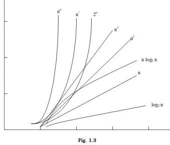
log2 n
n log2 n
n n2 n3 2n
n! nn
Fig. 1.3
The function that involves ‘n’ as an exponent, i.e., 2n, nn, n ! are called exponential
functions, which is too slow except for small size input function where growth is less than or equal to nc,(where ‘c’ is a constant) i.e.; n3, n2, n log
2n, n, log2 n are said to be polyno-mial. Algorithms with polynomial time can solve reasonable sized problems if the constant in the exponent is small.
When we analyze an algorithm it depends on the input data, there are three cases : 1. Best case
2. Average case 3. Worst case
In the best case, the amount of time a program might be expected to take on best possible input data.
In the average case, the amount of time a program might be expected to take on typical (or average) input data.
In the worst case, the amount of time a program would take on the worst possible input configuration.
1.8.3. AMSTRONG COMPLEXITY
itself. For example in a for loop there are 100 instructions in an if statement. If if condition is false then these 100 instructions will not be executed. If we apply the time complexity analysis in worst case, entire sequence is considered to compute the efficiency, which is an excessively large and unrealistic analysis of efficiency. But when we apply amortized complexity, the complexity is calculated when the instructions are executed (i.e., when if condition is true)
Here the time required to perform a sequence of (related) operations is averaged over all the operations performed. Amortized analysis can be used to show that the average cost of an operation is small, if one averages over a sequence of operations, even though a simple operation might be expensive. Amortized analysis guarantees the average perform-ance of each operation in the worst case.
1.9. TIME-SPACE TRADE OFF
There may be more than one approach (or algorithm) to solve a problem. The best algorithm (or program) to solve a given problem is one that requires less space in memory and takes less time to complete its execution. But in practice, it is not always possible to achieve both of these objectives. One algorithm may require more space but less time to complete its execution while the other algorithm requires less time space but takes more time to complete its execution. Thus, we may have to sacrifice one at the cost of the other. If the space is our constraint, then we have to choose a program that requires less space at the cost of more execution time. On the other hand, if time is our constraint such as in real time system, we have to choose a program that takes less time to complete its execu-tion at the cost of more space.
1.10. BIG “OH” NOTATION
Big Oh is a characteristic scheme that measures properties of algorithm complexity performance and/or memory requirements. The algorithm complexity can be determined by eliminating constant factors in the analysis of the algorithm. Clearly, the complexity function f(n) of an algorithm increases as ‘n’ increases.
Let us find out the algorithm complexity by analyzing the sequential searching algo-rithm. In the sequential search algorithm we simply try to match the target value against each value in the memory. This process will continue until we find a match or finish scanning the whole elements in the array. If the array contains ‘n’ elements, the maximum possible number of comparisons with the target value will be ‘n’ i.e., the worst case. That is the target value will be found at the nth position of the array.
f (n) = n
i.e., the worst case is when an algorithm requires a maximum number of iterations or steps to search and find out the target value in the array.
The best case is when the number of steps is less as possible. If the target value is found in a sequential search array of the first position (i.e., we need to compare the target value with only one element from the array)—we have found the element by executing only one iteration (or by least possible statements)
Average case falls between these two extremes (i.e., best and worst). If the target value is found at the n/2nd position, on an average we need to compare the target value with only half of the elements in the array, so
f (n) = n/2
The complexity function f(n) of an algorithm increases as ‘n’ increases. The function f (n)= O(n) can be read as “f of n is big Oh of n” or as “f (n) is of the order of n”. The total running time (or time complexity) includes the initializations and several other iterative statements through the loop.
The generalized form of the theorem is
f (n) = cknk + ck–1nk –1 + ck–2nk–2 + ... + c2n2 + c1n1 + c0n0
Where the constant ck > 0 Then, f (n) = O(nk)
Based on the time complexity representation of the big Oh notation, the algorithm can be categorized as :
1. Constant time O(1) 2. Logarithmic time Olog(n) 3. Linear time O(n)
4. Polynomial time O(nc)
5. Exponential time O(cn) Where c > 1
1.11. LIMITATION OF BIG “OH” NOTATION
Big Oh Notation has following two basic limitations :
1. It contains no effort to improve the programming methodology. Big Oh Notation does not discuss the way and means to improve the efficiency of the program, but it helps to analyze and calculate the efficiency (by finding time complexity) of the program.
2. It does not exhibit the potential of the constants. For example, one algorithm is taking 1000n2 time to execute and the other n3 time. The first algorithm is O(n2), which implies that it will take less time than the other algorithm which is O(n3). However in actual execution the second algorithm will be faster for n < 1000. We will analyze and design the problems in data structure. As we have discussed to develop a program of an algorithm, we should select an appropriate data structure for that algorithm.
1.12. CLASSIFICATION OF DATA STRUCTURE
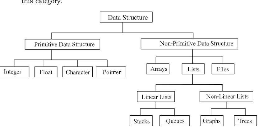
Data structures are broadly divided into two :
1.Primitive data structures : These are the basic data structures and are directly operated upon by the machine instructions, which is in a primitive level. They are integers, floating point numbers, characters, string constants, pointers etc. These primitive data structures are the basis for the discussion of more sophis-ticated (non-primitive) data structures in this book.
2.Non-primitive data structures : It is a more sophisticated data structure empha-sizing on structuring of a group of homogeneous (same type) or heterogeneous (different type) data items. Array, list, files, linked list, trees and graphs fall in this category.
Fig. 1.4. Classifications of data structures
The Fig. 1.4 will briefly explain other classifications of data structures. Basic opera-tions on data structure are to create a (non-primitive) data structure; which is considered to be the first step of writing a program. For example, in Pascal, C and C++, variables are created by using declaration statements.
int Int_Variable;
In C/C++, memory space is allocated for the variable “Int_Variable” when the above declaration statement executes. That is a data structure is created. Discussions on primitive data structures are beyond the scope of this book. Let us consider non-primitive data structures.
1.13. ARRAYS
Arrays are most frequently used in programming. Mathematical problems like ma-trix, algebra and etc can be easily handled by arrays. An array is a collection of homogene-ous data elements described by a single name. Each element of an array is referenced by a subscripted variable or value, called subscript or index enclosed in parenthesis. If an element of an array is referenced by single subscript, then the array is known as one dimensional array or linear array and if two subscripts are required to reference an ele-ment, the array is known as two dimensional array and so on. Analogously the arrays whose elements are referenced by two or more subscripts are called multi dimensional arrays.
1.13.1. ONE DIMENSIONAL ARRAY
1. The elements of the array are referenced respectively by an index set consisting of ‘n’ consecutive numbers.
2. The elements of the array are stored respectively in successive memory loca-tions.
‘n’ number of elements is called the length or size of an array. The elements of an array ‘A’ may be denoted in C as
A[0], A[1], A[2], ... A[n –1].
The number ‘n’ in A[n] is called a subscript or an index and A[n] is called a subscripted variable. If ‘n’ is 10, then the array elements A[0], A[1]...A[9] are stored in sequential memory locations as follows :
A[0] A[1] A[2] ... A[9]
In C, array can always be read or written through loop. To read a one-dimensional array, it requires one loop for reading and writing the array, for example:
For reading an array of ‘n’ elements for (i = 0; i < n; i ++) scanf (“%d”,&a[i]); For writing an array
for (i = 0; i < n; i ++) printf (“%d”, &a[i]); 1.13.2. MULTI DIMENSIONAL ARRAY
If we are reading or writing two-dimensional array, two loops are required. Similarly the array of ‘n’ dimensions would require ‘n’ loops. The structure of the two dimensional array is illustrated in the following figure :
int A[10][10];
A00 A01 A02 A08 A09
A10 A11 A19
A20
A30
A69
A70 A78 A79
A80 A81 A87 A88 A89
1.13.3. SPARSE ARRAYS
Sparse array is an important application of arrays. A sparse array is an array where nearly all of the elements have the same value (usually zero) and this value is a constant. One-dimensional sparse array is called sparse vectors and two-dimensional sparse arrays are called sparse matrix.
The main objective of using arrays is to minimize the memory space requirement and to improve the execution speed of a program. This can be achieved by allocating memory space for only non-zero elements.
For example a sparse array can be viewed as
0 0 8 0 0 0 0
0 1 0 0 0 9 0
0 0 0 3 0 0 0
0 31 0 0 0 4 0
0 0 0 0 7 0 0
Fig. 1.5. Sparse array
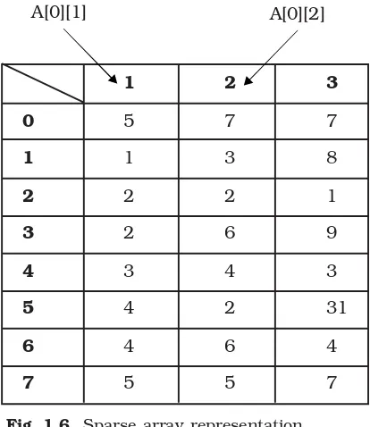
We will store only non-zero elements in the above sparse matrix because storing all the elements of the sparse array will be consisting of memory sparse. The non-zero ele-ments are stored in an array of the form.
A[0...n][1...3]
Where ‘n’ is the number of non-zero elements in the array. In the above Fig. 1.4 ‘n = 7’. The space array given in Fig. 1.4 may be represented in the array A[0...7][1...3].
1 2 3
0 5 7 7
1 1 3 8
2 2 2 1
3 2 6 9
4 3 4 3
5 4 2 31
6 4 6 4
7 5 5 7
Fig. 1.6. Sparse array representation
The element A[0][1] and A[0][2] contain the number of rows and columns of the sparse array. A[0][3] contains the total number of nonzero elements in the sparse array.
A[1][1] contains the number of the row where the first nonzero element is present in the sparse array. A[1][2] contains the number of the column of the corresponding nonzero element. A[1][3] contains the value of the nonzero element. In the Fig. 1.4, the first nonzero element can be found at 1st row in 3rd column.
1.14. VECTORS
A vector is a one-dimensional ordered collection of numbers. Normally, a number of contiguous memory locations are sequentially allocated to the vector. A vector size is fixed and, therefore, requires a fixed number of memory locations. A vector can be a column vector which represents a ‘n’ by 1 ordered collections, or a row vector which represents a 1 by ‘n’ ordered collections.
The column vector appears symbolically as follows :
A =
A row vector appears symbolically as follows : A = (A1, A2, A3, ... An)
Vectors can contain either real or complex numbers. When they contain real num-bers, they are sometime called real vectors. When they contain complex numnum-bers, they are called complex vectors.
1.15. LISTS
As we have discussed, an array is an ordered set, which consist of a fixed number of elements. No deletion or insertion operations are performed on arrays. Another main dis-advantage is its fixed length; we cannot add elements to the array. Lists overcome all the above limitations. A list is an ordered set consisting of a varying number of elements to which insertion and deletion can be made. A list represented by displaying the relation-ship between the adjacent elements is said to be a linear list. Any other list is said to be non linear. List can be implemented by using pointers. Each element is referred to as nodes; therefore a list can be defined as a collection of nodes as shown below :
x
Head1.16. FILES AND RECORDS
A file is typically a large list that is stored in the external memory (e.g., a magnetic disk) of a computer.
A record is a collection of information (or data items) about a particular entity. More specifically, a record is a collection of related data items, each of which is called a filed or attribute and a file is a collection of similar records.
Although a record is a collection of data items, it differs from a linear array in the following ways:
(a) A record may be a collection of non-homogeneous data; i.e., the data items in a record may have different data types.
(b) The data items in a record are indexed by attribute names, so there may not be a natural ordering of its elements.
1.17. CHARACTERISTICS OF STRINGS
In computer terminology the term ‘string’ refers to a sequence of characters. A finite set of sequence (alphabets, digits or special characters) of zero or more characters is called a string. The number of characters in a string is called the length of the string. If the length of the string is zero then it is called the empty string or null string.
1.17.1. STRING REPRESENTATION
Strings are stored or represented in memory by using following three types of struc-tures :
• Fixed length structures
• Variable length structures with fixed maximum • Linear structures
FIXED LENGTH REPRESENTATION. In fixed length storage each line is viewed as a record, where all records have the same length. That is each record accommodates maxi-mum of same number of characters.
The main advantage of representing the string in the above way is : 1. To access data from any given record easily.
2. It is easy to update the data in any given record. The main disadvantages are :
1. Entire record will be read even if most of the storage consists of inessential blank space. Time is wasted in reading these blank spaces.
2. The length of certain records will be more than the fixed length. That is certain records may require more memory space than available.
c P R O G R A M T O P R I N T ...
100 110 120
T W O I N T E G E R S ...
210 220 230
Fig. 1.9. Fixed length representation
Fig. 1.9 is a representation of input data (which is in Fig. 1.8) in a fixed length (records) storage media in a computer.
Variable Length Representation: In variable length representation, strings are stored in a fixed length storage medium. This is done in two ways.
1. One can use a marker, (any special characters) such as two-dollar sign ($$), to signal the end of the string.
2. Listing the length of the string at the first place is another way of representing strings in this method.
c p r o g r a m t o P r i n t t w o i n t e g e r s $$
Fig. 1.10. String representation using marker
31 c p r o g r a m t o p r i n t t w o i n t e g e r s
Fig. 1.11. String representation by listing the length
Linked List Representations: In linked list representations each characters in a string are sequentially arranged in memory cells, called nodes, where each node contain an item and link, which points to the next node in the list (i.e., link contain the address of the next node).
...
Fig. 1.12. One character per node
Fig. 1.13. Four character per node
We will discuss the implementation issues of linked list in chapter 5.
1.17.2. SUB STRING
Group of consecutive elements or characters in a string (or sentence) is called sub string. This group of consecutive elements may not have any special meaning. To access a sub string from the given string we need following information :
(a) Name of the string
(b) Position of the first character of the sub string in the given string (c) The length of the sub string
SELF REVIEW QUESTIONS
1. Explain how sparse matrix can be stored using arrays?
[Calicut - APR 1997 (BTech), MG - MAY 2002 (BTech) KERALA - MAY 2002 (BTech)] 2. Distinguish between time and space complexity?
[ANNA - MAY 2004 (MCA), MG - MAY 2004 (BTech)] 3. Discuss the performance analysis and evaluation methods of algorithm?
[KERALA - DEC 2004 (BTech), MG - MAY 2004 (BTech)] 4. Define and explain Big O notation?
[MG - NOV 2004 (BTech), MG - NOV 2003 (BTech)] 5. What are sparse matrixes? Give an example?
[CUSAT - NOV 2002 (BTech), Calicut - APR 1995 (BTech), CUSAT - JUL 2002 (MCA), MG - NOV 2004 (BTech) KERALA - MAY 2001 (BTech), KERALA - MAY 2003 (BTech)] 6. Explain the schemes of data representations for strings? [MG - NOV 2004 (BTech)] 7. Define complexity of an algorithm. What is meant by time-space trade off ?
[CUSAT - MAY 2000 (BTech), MG - NOV 2004 (BTech), KERALA - DEC 2002 (BTech), MG - MAY 2000 (BTech)] 8. Discuss the different steps in the development of an algorithm?
[MG - NOV 2004 (BTech)] 9. Discuss the advantages and disadvantages of Modular Programming.
[Calicut - APR 1995 (BTech)] 10. What is an Algorithm? Explain with example the time and space analysis of an
algo-rithm. [Calicut - APR 1995 (BTech)]
11. Pattern matching in strings. [Calicut - APR 1997 (BTech)] 12. Distinguish between primitive and non-primitive data structures. Explain how integer data are mapped to storage. [CUSAT - APR 1998 (BTech)] 13. Explain what is meant by dynamic storage management?
[ANNA - DEC 2004 (BE), CUSAT - MAY 2000 (BTech)] 14. Explain in detail about top-down approach and bottom-up approach with suitable pro-gramming examples. [ANNA - MAY 2003 (BE), ANNA - DEC 2003 (BE)] 15. What do you mean by stepwise refinement?
[KERALA - DEC 2004 (BTech), ANNA - DEC 2003 (BE) KERALA - DEC 2003 (BTech), KERALA - JUN 2004 (BTech) KERALA - MAY 2003 (BTech)] 16. What are the features of structured programming methodologies? Explain.
[ANNA - MAY 2003 (BE), ANNA - DEC 2004 (BE)] 17. Differentiate linear and non-linear data structures.
20. What is meant by algorithm ? What are its measures? [ANNA - MAY 2004 (BE)] 21. What are primitive data types ? [ANNA - MAY 2003 (BE)] 22. Explain (i) Array vs. record. (ii) Time complexity
[KERALA - MAY 2001 (BTech), KERALA - JUN 2004 (BTech)] 23. Explain Programming methodology. [KERALA - DEC 2003 (BTech)] 24. Explain about analysis of algorithms.
[KERALA - MAY 2003 (BTech), KERALA - DEC 2003 (BTech)] 25. What is structured programming ? Explain. [KERALA - MAY 2001 (BTech)] 26. Distinguish between a program and an algorithm. [KERALA - MAY 2002 (BTech)] 27. Explain the advantages and disadvantage of list structure over array structure.
[KERALA - MAY 2002 (BTech)] 28. Explain the term “data structure”. [KERALA - NOV 2001 (BTech)] 29. What do you understand by best, worst and average case analysis of an algorithm ?
[KERALA - NOV 2001 (BTech)] 30. What are the uses of an array ? What is an ordered array ?
18
2
Memory Management
A memory or store is required in a computer to store programs (or information or data). Data used by the variables in a program is also loaded into memory for fast access. A memory is made up of a large number of cells, where each cell is capable of storing one bit. The cells may be organized as a set of addressable words, each word storing a se-quence of bits. These addressable memory cells should be managed effectively to increase its utilization. That is memory management is to handle request for storage (that is new memory allocations for a variable or data) and release of storage (or freeing the memory) in most effective manner. While designing a program the programmer should concentrate on to allocate memory when it is required and to deallocate once its use is over.
In other words, dynamic data structure provides flexibility in adding, deleting or rearranging data item at run-time. Dynamic memory management techniques permit us to allocate additional memory space or to release unwanted space at run-time, thus optimizing the use of storage space. Next topic will give you a brief introduction about the storage management, static as well as dynamic functions available in C.
2.1. MEMORY ALLOCATION IN C
There are two types of memory allocations in C: 1. Static memory allocation or Compile time 2. Dynamic memory allocation or Run time
In static or compile time memory allocations, the required memory is allocated to the variables at the beginning of the program. Here the memory to be allocated is fixed and is determined by the compiler at the compile time itself. For example
int i, j; //Two bytes per (total 2) integer variables
float a[5], f; //Four bytes per (total 6) floating point variables When the first statement is compiled, two bytes for both the variable ‘i’ and ‘j’ will be allocated. Second statement will allocate 20 bytes to the array A [5 elements of floating point type, i.e., 5 × 4] and four bytes for the variable ‘f ’. But static memory allocation has following drawbacks.
If you try to read 15 elements, of an array whose size is declared as 10, then first 10 values and other five consecutive unknown random memory values will be read. Again if you try to assign values to 15 elements of an array whose size is declared as 10, then first 10 elements can be assigned and the other 5 elements cannot be assigned/accessed.
to other applications (or process which is running parallel to the program) and its status is set as allocated and not free. This leads to the inefficient use of memory.
The dynamic or run time memory allocation helps us to overcome this problem. It makes efficient use of memory by allocating the required amount of memory whenever is needed. In most of the real time problems, we cannot predict the memory requirements. Dynamic memory allocation does the job at run time.
C provides the following dynamic allocation and de-allocation functions : (i) malloc( ) (ii) calloc( )
(iii) realloc( ) (iv) free( )
2.1.1. ALLOCATING A BLOCK OF MEMORY
The malloc( ) function is used to allocate a block of memory in bytes. The malloc function returns a pointer of any specified data type after allocating a block of memory of specified size. It is of the form
ptr = (int_type *) malloc (block_size)
‘ptr’ is a pointer of any type ‘int_type’ byte size is the allocated area of memory block. For example
ptr = (int *) malloc (10 * sizeof (int));
On execution of this statement, 10 times memory space equivalent to size of an ‘int’ byte is allocated and the address of the first byte is assigned to the pointer variable ‘ptr’ of type ‘int’.
Remember the malloc() function allocates a block of contiguous bytes. The alloca-tion can fail if the space in the heap is not sufficient to satisfy the request. If it fails, it returns a NULL pointer. So it is always better to check whether the memory allocation is successful or not before we use the newly allocated memory pointer. Next program will illustrate the same.
PROGRAM 2.1
//THIS IS A PROGRAM TO FIND THE SUM OF n ELEMENTS USING //DYNAMIC MEMORY ALLOCATION
#include<stdio.h> #include<conio.h> #include<process.h>
//Defining the NULL pointer as zero
#define NULL 0
void main() {
int i,n,sum;
clrscr(); //Clear the screen
printf(“\nEnter the number of the element(s) to be added = ”); scanf(“%d”,&n); //Enter the number of elements
//Allocating memory space for n integers of int type to *ptr ptr=(int *)malloc(n*sizeof(int));
//Checking whether the memory is allocated successfully if(ptr == NULL)
{
printf(“\n\nMemory allocation is failed”); exit(0);
}
//Reading the elements to the pointer variable *ele for(ele=ptr,i=1;ele<(ptr+n);ele++,i++)
{
printf(“Enter the %d element = ”,i); scanf(“%d”,ele);
}
//Finding the sum of n elements for(ele=ptr,sum=0;ele<(ptr+n);ele++)
sum=sum+(*ele);
printf(“\n\nThe SUM of no(s) is = %d”,sum); getch();
}
Similarly, memory can be allocated to structure variables. For example struct Employee
{
int Emp_Code; char Emp_Name[50]; float Emp_Salary; };
Here the structure is been defined with three variables. struct Employee *str_ptr;
str_ptr = (struct Employee *) malloc(sizeof (struct Employee));
2.1.2. ALLOCATING MULTIPLE BLOCKS OF MEMORY
The calloc() function works exactly similar to malloc() function except for the fact that it needs two arguments as against one argument required by malloc() function. While malloc() function allocates a single block of memory space, calloc() function allocates mul-tiple blocks of memory, each of the same size, and then sets all bytes to zero. The general form of calloc() function is
ptr = (int_type*) calloc(n sizeof (block_size)); ptr = (int_type*) malloc(n* (sizeof (block_size));
The above statement allocates contiguous space for ‘n’ blocks, each of size of block_size bytes. All bytes are initialized to zero and a pointer to the first byte of the allocated memory block is returned. If there is no sufficient memory space, a NULL pointer is returned. For example
ptr = (int *) calloc(25, 4);
ptr = (int *) calloc(25,sizeof (float));
Here, in the first statement the size of data type in byte for which allocation is to be made (4 bytes for a floating point numbers) is specified and 25 specifies the number of elements for which allocation is to be made.
Note : The memory allocated using malloc() function contains garbage values, the memory allocated by calloc() function contains the value zero.
2.1.3. RELEASING THE USED SPACE
Dynamic memory allocation allocates block(s) of memory when it is required and deallocates or releases when it is not in use. It is important and is our responsibility to release the memory block for future use when it is not in use, using free() function.
The free() function is used to deallocate the previously allocated memory using malloc() or calloc() function. The syntax of this function is
free(ptr);
‘ptr’ is a pointer to a memory block which has already been allocated by malloc() or calloc() functions. Trying to release an invalid pointer may create problems and cause system crash.
2.1.4. RESIZE THE SIZE OF A MEMORY BLOCK
In some situations, the previously allocated memory is insufficient to run the cor-rect application, i.e., we want to increase the memory space. It is also possible that the memory allocated is much larger than necessary, i.e., we want to reduce the memory space. In both the cases we want to change the size of the allocated memory block and this can be done by realloc() function. This process is called reallocation of the memory. The syntax of this function is
ptr = realloc(ptr, New_Size)
Where ‘ptr’ is a pointer holding the starting address of the allocated memory block. And New_Size is the size in bytes that the system is going to reallocate. Following example will elaborate the concept of reallocation of memory.
ptr = (int *) realloc(ptr, sizeof (int));
ptr = (int *) realloc(ptr, 2); Both the statements are same
ptr = (int *) realloc(ptr, sizeof (float));
ptr = (int *) realloc(ptr, 4); Both the statements are same
2.2. DYNAMIC MEMORY ALLOCATION IN C++
Although C++ supports all the functions (i.e., malloc, calloc, realloc and free) used in C, it also defines two unary operators new and delete that performs the task of allocating and freeing the memory in a better and easier way.
An object (or variable) can be created by using new, and destroyed by using delete, as and when required. A data object created inside a block with new, will remain in exist-ence until it is explicitly destroyed by using delete. Thus, the lifetime of an object is di-rectly under our control and is unrelated to the block structure of the program.
The new operator can be used to create objects of any type. It takes the following general form:
Pointer_Variable = new data_type;
Here, Pointer_Variable is a pointer of type data_type. The new operator allocates sufficient memory to hold a data object of type data_type and returns the address of the object. The data_type may be any valid data type. The Pointer_Variable holds the address of the memory space allocated. For example:
int *Var1 = new int; float *Var2 = new float;
Where Var1 is a pointer of type int and Var2 is a pointer of type float.
When a data object is no longer needed, it is destroyed to release the memory space for reuse. The general form of its use is:
delete Pointer_Variable;
The Pointer_Variable is the pointer that points to a data object created with new. delete Var1;
delete Var2
2.3. FREE STORAGE LIST
Now we have discussed several functions to allocate and freeing storage (or deallocate). To store any data, memory space is allocated dynamically using the function we have discussed in the earlier sections. That is storage allocation is done when the programmer requests it by declaring a structure at the run time.
But freeing storage is not as easy as allocation. When a program or block of program (or function or module) ends, the storage allocated at the beginning of the program will be freed. Dynamically a memory cell can be freed using the operator delete in C++.
Two problems arise in the context of storage release. One is the accumulation of garbage (called garbage collection) and another is that of dangling reference, which is dis-cussed in following sections.
2.4. GARBAGE COLLECTION
Suppose some memory space becomes reusable when a node (or a variable) is de-leted from a list or an entire list is dede-leted from a program. Obviously, we would like the space to be made available for future use. One way to bring this about is to immediately reinsert the space into the free-storage list-using delete or free. However, this method may be too time-consuming for the operating system and most of the programming languages, reserve themselves the task of storage release, even if they provide operator like delete. So the problem arises when the system considers a memory cell as free storage.
The operating system of a computer may periodically collect all the deleted space onto the free-storage list. Any technique that does this is called garbage collection. Gar-bage collection usually takes place in two steps. First the computer runs through all lists, tagging those cells which are currently in use, and then the computer runs through the memory, collecting all untagged space onto the free-storage list. The garbage collection may take place when there is only some minimum amount of space or no space at all left in the free-storage list, or when the CPU is idle and has time to do the collection. Generally speaking, the garbage collection is invisible to the programmer. Any future discussion about this topic of garbage collection lies beyond the scope of this text.
2.5. DANGLING REFERENCE
A dangling reference is a pointer existing in a program, which still accesses a block of memory that has been freed. For example consider the following code in C++.
---Here temp is the dangling reference. temp is a pointer which is pointing to a memory block ptr, which is just deleted. This can be overcome by using a reference counters.
2.6. REFERENCE COUNTERS
In the reference-counter method, a counter is kept that records how many pointers have direct access to each memory block. When a memory block is first allocated, its reference counter is set to 1. Each time another link is made pointing to this block, the reference counter is incremented. Each time a link to its block is broken, the reference counter is decremented. When the count reaches 0, the memory block is not accessed by any other pointer and it can be returned to the free list. This technique completely elimi-nates the dangling reference problem.
2.7. STORAGE COMPACTION
Storage compaction is another technique for reclaiming free storage. Compaction works by actually moving blocks of data from one location in the memory to another so as to collect all the free blocks into one single large block. Once this single block gets too small again, the compaction mechanism is called gain to reclaim the unused storage. Here no storage releasing mechanism is used. Instead, a marking algorithm is used to mark blocks that are still in use. Then instead of freeing each unmarked block by calling a release mechanism to put it on the free list, the compactor simply collects all unmarked blocks into one large block at one end of the memory segment.
2.8. BOUNDARY TAG METHOD
Boundary tag representation is a method of memory management described by Knuth. Boundary tags are data structures on the boundary between blocks in the heap from which memory is allocated. The use of such tags allow blocks of arbitrary size to be used as shown in the Fig. 2.1.
Suppose ‘n’ bytes of memory are to be allocated from a large area, in contiguous blocks of varying size, and that no form of compaction or rearrangement of the allocated segments will be used.
To reserve a block of ‘n’ bytes of memory, a free space of size ‘n’ or larger must be located. If we could locate a large size memory, then the allocation process will divide it into an allocated space, and a new smaller free space. Suppose free space is subdivided in this manner several times, and some of the allocated regions are “released” (after use i.e., deallocated).
If we try to reserve more memory; even though there is a large contiguous chunk of free space, the memory manager perceives it as two smaller segments and so may falsely conclude that it has insufficient free space to satisfy a large request.
For optimal use of the memory, adjacent free segments must be combined. For maximum availability, they must be combined as soon as possible. The task of identifying and merging adjacent free segments should be done when a segment is released, called the boundary tag method. The method consistently applied to ensure that there would never be two adjacent free segments. This guarantees the largest available free space short of compacting the string space.
SELF REVIEW QUESTIONS
1. Explain the representation of array in memory. [MG - MAY 2004 (BTech)] 2. Write a note on garbage collection and compaction.
[MG - NOV 2003 (BTech), MG - MAY 2000 (BTech)] 3. Discuss the garbage collection techniques and drawbacks of each.
[MG - MAY 2002 (BTech)] 4. Write note on storage allocation and storage release. [MG - MAY 2002 (BTech)] 5. Explain the different storage representations for string.
[KERALA - MAY 2001 (BTech), CUSAT - MAY 2000 (BTech)] 6. What is the need for Garbage collection? Explain a suitable data structure to implement
Garbage collection. [CUSAT - NOV 2002 (BTech)]
7. Write a note on Storage Management. [ANNA - DEC 2004 (BE)] 8. Explain about free storage lists. [KERALA - DEC 2004 (BTech)] 9. Explain Storage Compaction. [KERALA - JUN 2004 (BTech)] 10. Explain Garbage Collection. [KERALA - DEC 2003 (BTech)] 11. What are reference counters ? [KERALA - MAY 2001 (BTech)] 12. Explain about boundary tag method. [KERALA - MAY 2001 (BTech)] 13. Write in detail the garbage collection and the compaction process.
The Stack
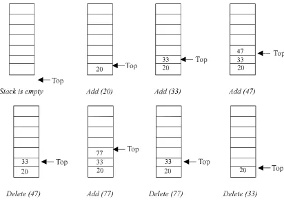
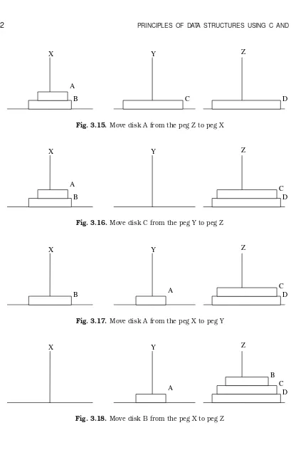
A stack is one of the most important and useful non-primitive linear data structure in computer science. It is an ordered collection of items into which new data items may be added/inserted and from which items may be deleted at only one end, called the top of the stack. As all the addition and deletion in a stack is done from the top of the stack, the last added element will be first removed from the stack. That is why the stack is also called Last-in-First-out(LIFO). Note that the most frequently accessible element in the stack is the top most elements, whereas the least accessible element is the bottom of the stack. The operation of the stack can be illustrated as in Fig. 3.1.
Fig. 3.1. Stack operation.
The insertion (or addition) operation is referred to as push, and the deletion (or remove) operation as pop. A stack is said to be empty or underflow, if the stack contains no
26
elements. At this point the top of the stack is present at the bottom of the stack. And it is overflow when the stack becomes full, i.e., no other elements can be pushed onto the stack. At this point the top pointer is at the highest location of the stack.
3.1. OPERATIONS PERFORMED ON STACK
The primitive operations performed on the stack are as follows:
PUSH: The process of adding (or inserting) a new element to the top of the stack is called PUSH operation. Pushing an element to a stack will add the new element at the top. After every push operation the top is incremented by one. If the array is full and no new element can be accommodated, then the stack overflow condition occurs.
POP: The process of deleting (or removing) an element from the top of stack is called POP operation. After every pop operation the stack is decremented by one. If there is no element in the stack and the pop operation is performed then the stack underflow condi-tion occurs.
3.2. STACK IMPLEMENTATION
Stack can be implemented in two ways: 1. Static implementation (using arrays) 2. Dynamic implementation (using pointers)
Static implementation uses arrays to create stack. Static implementation using arrays is a very simple technique but is not a flexible way, as the size of the stack has to be declared during the program design, because after that, the size cannot be varied (i.e., increased or decreased). Moreover static implementation is not an efficient method when resource optimization is concerned (i.e., memory utilization). For example a stack is imple-mented with array size 50. That is before the stack operation begins, memory is allocated for the array of size 50. Now if there are only few elements (say 30) to be stored in the stack, then rest of the statically allocated memory (in this case 20) will be wasted, on the other hand if there are more number of elements to be stored in the stack (say 60) then we cannot change the size array to increase its capacity.
The above said limitations can be overcome by dynamically implementing (is also called linked list representation) the stack using pointers.
3.3. STACK USING ARRAYS
Implementation of stack using arrays is a very simple technique. Algorithm for push-ing (or add or insert) a new element at the top of the stack and popppush-ing (or delete) an element from the stack is given below.
Algorithm for push
1. If TOP = SIZE – 1, then:
(a) Display “The stack is in overflow condition” (b) Exit
2. TOP = TOP + 1 3. STACK [TOP] = ITEM 4. Exit
Algorithm for pop
Suppose STACK[SIZE] is a one dimensional array for implementing the stack, which will hold the data items. TOP is the pointer that points to the top most element of the stack. DATA is the popped (or deleted) data item from the top of the stack.
1. If TOP < 0, then
(a) Display “The Stack is empty” (b) Exit
2. Else remove the Top most element 3. DATA = STACK[TOP]
4. TOP = TOP – 1 5. Exit
PROGRAM 3.1
//THIS PROGRAM IS TO DEMONSTRATE THE OPERATIONS PERFORMED //ON THE STACK AND IT IS IMPLEMENTATION USING ARRAYS
//CODED AND COMPILED IN TURBO C
#include<stdio.h> #include<conio.h>
//Defining the maximum size of the stack #define MAXSIZE 100
//Declaring the stack array and top variables in a structure struct stack
{
int stack[MAXSIZE]; int Top;
};
//type definition allows the user to define an identifier that would //represent an existing data type. The user-defined data type identifier //can later be used to declare variables.
//This function will add/insert an element to Top of the stack void push(NODE *pu)
{
int item;
//if the top pointer already reached the maximum allowed size then //we can say that the stack is full or overflow
if (pu->Top == MAXSIZE–1) {
printf(“\nThe Stack Is Full”); getch();
}
//Otherwise an element can be added or inserted by //incrementing the stack pointer Top as follows else
{
printf(“\nEnter The Element To Be Inserted = ”); scanf(“%d”,&item);
pu->stack[++pu->Top]=item; }
}
//This function will delete an element from the Top of the stack void pop(NODE *po)
{
int item;
//If the Top pointer points to NULL, then the stack is empty //That is NO element is there to delete or pop
if (po->Top == -1)
printf(“\nThe Stack Is Empty”);
//Otherwise the top most element in the stack is popped or //deleted by decrementing the Top pointer
else {
item=po->stack[po->Top--];
printf(“\nThe Deleted Element Is = %d”,item); }
}
//This function to print all the existing elements in the stack void traverse(NODE *pt)
{
int i;
//That is NO element is there to delete or pop if (pt->Top == -1)
printf(“\nThe Stack is Empty”);
//Otherwise all the elements in the stack is printed else
{
printf(“\n\nThe Element(s) In The Stack(s) is/are...”); for(i=pt->Top; i>=0; i--)
//Declaring an pointer variable to the structure NODE *ps;
//Initializing the Top pointer to NULL ps->Top=–1;
do {
clrscr();
//A menu for the stack operations printf(“\n1. PUSH”);
printf(“\n2. POP”); printf(“\n3. TRAVERSE”); printf(“\nEnter Your Choice = ”); scanf (“%d”, &choice);
switch(choice) {
case 1://Calling push() function by passing //the structure pointer to the function push(ps);
break;
case 2://calling pop() function pop(ps);
break;
case 3://calling traverse() function traverse(ps);
default:
printf(“\nYou Entered Wrong Choice”) ; }
printf(“\n\nPress (Y/y) To Continue = ”); //Removing all characters in the input buffer //for fresh input(s), especially <<Enter>> key fflush(stdin);
scanf(“%c”,&ch); }while(ch == 'Y' || ch == 'y'); }
PROGRAM 3.2
//THIS PROGRAM IS TO DEMONSTRATE THE OPERATIONS //PERFORMED ON STACK & IS IMPLEMENTATION USING ARRAYS //CODED AND COMPILED IN TURBO C++
#include<iostream.h> #include<conio.h>
//Defining the maximum size of the stack #define MAXSIZE 100
//A class initialized with public and private variables and functions class STACK_ARRAY
{
int stack[MAXSIZE]; int Top;
public:
//constructor is called and Top pointer is initialized to –1 //when an object is created for the class
STACK_ARRAY() {
Top=–1; }
//This function will add/insert an element to Top of the stack void STACK_ARRAY::push()
{
int item;
//if the top pointer already reached the maximum allowed size then //we can say that the stack is full or overflow
if (Top == MAXSIZE–1) {
cout<<“\nThe Stack Is Full”; getch();
}
//Otherwise an element can be added or inserted by //incrementing the stack pointer Top as follows else
{
cout<<“\nEnter The Element To Be Inserted = ”; cin>>item;
stack[++Top]=item; }
}
//This function will delete an element from the Top of the stack void STACK_ARRAY::pop()
{
int item;
//If the Top pointer points to NULL, then the stack is empty //That is NO element is there to delete or pop
if (Top == –1)
cout<<“\nThe Stack Is Empty”;
//Otherwise the top most element in the stack is poped or //deleted by decrementing the Top pointer
else {
item=stack[Top--];
cout<<“\nThe Deleted Element Is = ”<<item; }
}
//This function to print all the existing elements in the stack void STACK_ARRAY::traverse()
int i;
//If the Top pointer points to NULL, then the stack is empty //That is NO element is there to delete or pop
if (Top == -1)
cout<<“\nThe Stack is Empty”;
//Otherwise all the elements in the stack is printed else
{
cout<<“\n\nThe Element(s) In The Stack(s) is/are...”; for(i=Top; i>=0; i--)
cout<<“\n ”<<stack[i]; }
}
void main() {
int choice; char ch;
//Declaring an object to the class STACK_ARRAY ps;
do {
clrscr();
//A menu for the stack operations cout<<“\n1. PUSH”;
cout<<“\n2. POP”; cout<<“\n3. TRAVERSE”; cout<<“\nEnter Your Choice = ”; cin>>choice;
switch(choice) {
case 1://Calling push() function by class object ps.push();
break;
case 2://calling pop() function ps.pop();
case 3://calling traverse() function ps.traverse();
break;
default:
cout<<“\nYou Entered Wrong Choice” ; }
cout<<“\n\nPress (Y/y) To Continue = ”; cin>>ch;
}while(ch == ‘Y’ || ch == ‘y’); }
3.4. APPLICATIONS OF STACKS
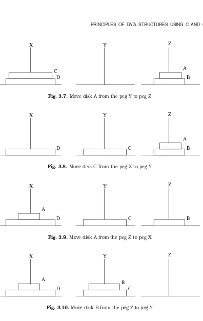
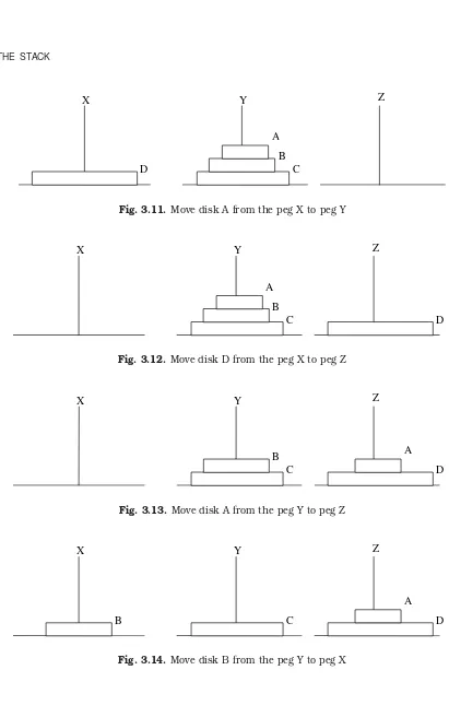
There are a number of applications of stacks; three of them are discussed briefly in the preceding sections. Stack is internally used by compiler when we implement (or ex-ecute) any recursive function. If we want to implement a recursive function non-recursively, stack is programmed explicitly. Stack is also used to evaluate a mathematical expression and to check the parentheses in an expression.
3.4.1. RECURSION
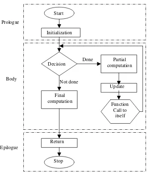
Recursion occurs when a function is called by itself repeatedly; the function is called recursive function. The general algorithm model for any recursive function contains the following steps:
1.Prologue: Save the parameters, local variables, and return address.
2.Body: If the base criterion has been reached, then perform the final computation and go to step 3; otherwise, perform the partial computation and go to step 1 (initiate a recursive call).
3.Epilogue: Restore the most recently saved parameters, local variables, and re-turn address.
A flowchart model for any recursive algorithm is given in Fig. 3.2.
Start
Stop Initialization
Decision Done computationPartial
Final computation
Function Call to
itself Not done
Update
Return Prologue
Body
Epilogue
Fig. 3.2. Flowchart model for a recursive algorithm
The Last-in-First-Out characteristics of a recursive function points that the stack is the most obvious data structure to implement the recursive function. Programs compiled in modern high-level languages (even C) make use of a stack for the procedure or function invocation in memory. When any procedure or function is called, a number of words (such as variables, return address and other arguments and its data(s) for future use) are pushed onto the program stack. When the procedure or function returns, this frame of data is popped off the stack.
The stack is a region of main memory within which programs temporarily store data as they execute. For example, when a program sends parameters to a function, the param-eters are placed on the stack. When the function completes its execution these paramparam-eters are popped off from the stack. When a function calls other function the current contents (ie., variables) of the caller function are pushed onto the stack with the address of the instruction just next to the call instruction, this is done so after the execution of called function, the compiler can backtrack (or remember) the path from where it is sent to the called function.
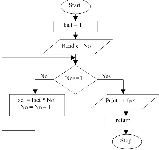
The recursive mechanism can be best described by an example. Consider the follow-ing program to calculate factorial of a number recursively, which explicitly describes the recursive framework.
PROGRAM 3.3
//PROGRAM TO FIND FACTORIAL OF A NUMBER, RECURSIVELY
#include<conio.h> #include<iostream.h>
void fact(int no, int facto) {
if (no <= 1) {
//Final computation and returning and restoring address cout<<“\nThe Factorial is = ”<<facto;
return; }
else {
//Partiial computation of the program facto=facto*no;
//Function call to itself, that is recursion fact(--no,facto);
}
}
void main() {
clrscr();
//Initialization of formal parameters, local variables and etc. factorial=1;
cout<<“\nEnter the No = ”; cin>>number;
//Starting point of the function, which calls itself fact(number,factorial);
getch(); }
Fig. 3.3. Flowchart for finding factorial recursively 3.4.2. RECURSION vs ITERATION
Recursion of course is an elegant programming technique, but not the best way to solve a problem, even if it is recursive in nature. This is due to the following reasons:
1. It requires stack implementation.
2. It makes inefficient utilization of memory, as every time a new recursive call is made a new set of local variables is allocated to function.
3. Moreover it also slows down execution speed, as function calls require jumps, and saving the current state of program onto stack before jump.