ADAMA BAH
TNP2K WORKING PAPER 01 – 2013
September 2013
FINDING THE BEST INDICATORS TO
3
ADAMA BAH
TNP2K WORKING PAPER 01 – 2013
September 2013
TNP2K Working Papers Series disseminates the findings of work in progress to encourage discussion and exchange of
ideas on poverty, social protection and development issues. The publication of this series is supported by the
Government of Australia through the Poverty Reduction Support Facility (PRSF), for the Government of Indonesia’s National
Team for Accelerating Poverty Reduction (TNP2K).
The findings, interpretations and conclusions herein are those of the author(s) and do not necessarily reflect the views of the
Government of Australia or the Government of Indonesia.
The text and data in this publication may be reproduced as long as the source is cited. Reproductions for commercial
purposes are forbidden.
Suggestion to cite: Bah, Adama (2013), ‘Finding the Best Indicators to Identify the Poor’, TNP2K Working Paper 01-2013.
Tim Nasional Percepatan Penanggulangan Kemiskinan (TNP2K): Jakarta, Indonesia.
To request copies of the paper or for more information on the series, please contact the TNP2K - Knowledge Management
Unit (kmu@tnp2k.go.id).
Papers are also available on the TNP2K’s website (www.tnp2k.go.id)
TNP2K
Email: info@tnp2k.go.id :: tnp2k@wapresri.go.id
Tel: 021 391 2812
4
FINDING THE BEST INDICATORS TO IDENTIFY THE POOR
Adama Bah
1September 2013
Abstract
Proxy-means testing (PMT) is a method used to assess household or individual welfare level based on
a set of observable indicators. The accuracy, and therefore usefulness of PMT relies on the selection
of indicators that produce accurate predictions of household welfare. In this paper I propose a method
to identify indicators that are robustly and strongly correlated with household welfare, measured by
per capita consumption. From an initial set of 340 candidate variables drawn from the Indonesian
Family Life Survey, I identify the variables that contribute most significantly to model predictive
performance and that are therefore desirable to be included in a PMT formula. These variables span
the categories of household private asset holdings, access to basic domestic energy, education level,
sanitation and housing. A comparison of the predictive performance of PMT formulas including 10,
20 and 30 of the best predictors of welfare shows that leads to recommending formulas with 20
predictors. Such parsimonious models have similar predictive performance as the PMT formulas
currently used in Indonesia, although these latter are based on models of 32 variables on average.
Keywords: Proxy-Means Testing, Variable/Model Selection, Targeting, Poverty, Social Protection.
JEL codes: I38, C52.
1
The National Team for the Acceleration of Poverty Reduction (TNP2K), Indonesia Vice-President Office, and CERDI-University of Auvergne, France – Email: adamabah@gmail.com
5
“The essential ingredients [of specification searches] are judgment and purpose, which jointly
determine where in a data set one ought to be digging and also which stones are gems and which are rocks.”
E. E. Leamer (1978)
Introduction
Proxy-means tests (PMT) have been increasingly used to identify poor households in developing
countries. PMT deals with the following problem, which is a typical situation in most developing
countries. There is no official registry that contains accurate and up to date information on household
and/or individual revenue. Self-reported income is therefore unverifiable, and it can be potentially
time consuming and costly to identify the poor. Proxy-means testing (PMT) allows assessing
household welfare based on observable indicators.
The implementation of PMT requires two distinct data sources. First, a household survey containing
information on household expenditures (or income) and socioeconomic characteristics is required. It
is used to estimate the correlation between household consumption, and a set of observable
characteristics based on simple regression methods.2 The set of weights (coefficients) derived from
these consumption regressions provides a scoring formula, which is used to compute “PMT scores”,
or predicted consumption, in a targeting survey.3 A targeting survey, or “census of the poor”, is
administered to all households or individuals considered as potentially eligible for social protection
programs. It collects information on socioeconomic indicators that enter the PMT formula estimated
using the household consumption survey.
The accuracy, and therefore the usefulness of PMT for targeting social programs, depends critically
on the quality of the indicators available in the targeting survey: they need to be good predictors of
welfare or poverty. In addition, such predictors need to be easy to collect and verify,4 as well as
2
See Sumarto et al. (2007) for a discussion of the consumption regression approach used for PMT in comparison with alternative approaches to estimating household welfare with the objective to identify the poor.
3
A similar approach is also used to develop “small area estimation poverty maps”, following the method proposed by Elbers
et al. (2003). The difference is that the second data source used for poverty maps is typically a population census.
4
6 limited in number, given that targeting survey interviews should be short. In the context of the
implementation of a PMT method for targeting social protection programs, the key issue is therefore
to identify among a large set of candidate variables the predictors that are cost-effective to be included
in the targeting survey because they are reliable in producing good predictions of household welfare.
It is not straightforward to identify good predictors of welfare. For a number K of candidate variables,
the data set does not “admit a unique set of inferences” (Leamer 1985). Instead, the model space is
“infinite dimensional” (Leamer 1983): there are 2K possible models (with different sets of predictors)
that can be estimated. When K is larger than 30, there are billions of possible models: it is impossible
to find the single best one. Moreover, among all possible models, there are a large number of models
that provide good predictions, which is acknowledged in the method developed in this chapter.
Through random sampling of models from the entire model space, this method allows first assessing
the level of predictive performance that can be expected from a good model, and then identifying
which variables are more likely to produce such models.
The model random sampling method relates to the “sensitivity analyses” advocated by Leamer (1985)
to address model uncertainty.5 The robustness of a variable is assessed here by evaluating whether
changes in the set of predictors with which this variable is combined lead to differences in the
contribution of this variable to model predictive performance. In the literature, a number of analyses
of the sensitivity of model parameters to changes in assumptions, in particular to changes in the set of
predictors, have been conducted using the extreme-bounds tests proposed by Leamer6 – see e.g.
Levine and Renelt (1992). However, this approach has been criticized, for instance by Granger and
Uhlig (1990) and Sala-i-Martin (1997), for giving the same importance (weight) to all models. Indeed,
some models are obviously not “likely to be the true model” (Sala-i-Martin 1997), in the sense that
they have a weak performance. Therefore, the robustness of a variable should not be rejected based on
being updated, as households might have made the link between being surveyed and receiving benefits. The indicators selected for the targeting survey should therefore be easily verifiable by the enumerators and the risk of measuring them with error should be low.
5
Leamer discusses the need for sensitivity analyses to assess the robustness of the empirical relationship between a given variable or set of variables and the outcome of interest. The sensitivity analysis approach and debate have mostly been limited to the macroeconomic literature, in particular the cross-country growth literature.
6
7 such models. Instead it is recommended to “restrict attention to better fitting models” (Sala-i-Martin et
al. 2004), which is the approach adopted in this chapter.
I implement the model random sampling method on a set of 340 indicators drawn from the 2007
Indonesian Family Life Survey. These indicators are subsequently ranked according to their
probability of being included in good predictive models and to their contribution to the predictive
performance of these models. I find as good predictors of welfare, and therefore useful in both a
targeting survey and a PMT formula, variables that span the categories of private asset holdings,
access to basic domestic energy, education level, sanitation and housing. The model random sampling
method leaves the decision regarding the predictors to be used in both the targeting survey and the
PMT formulas to the researcher and/or the policymaker. Yet, it provides them with useful information
to make this decision in a transparent manner, such as the expected increase in predictive performance
from the inclusion of a given variable.
The prediction accuracy that can be expected from PMT formulas that include the best predictors of
welfare is discussed, to illustrate the use of the results in terms of predictor ranking. In particular,
comparing the predictive performance of models with 10, 20 and 30 of the best variables, I find
overall that good predictions are obtained with 20 predictors and therefore recommend using such
parsimonious models. These results contribute to the literature on targeting social programs by further
demonstrating that targeting using PMT has inherent relatively important errors, even when including
a large number of good predictors. Therefore, it is recommended that PMT is used in combination
with other targeting methods, in line with Coady et al. (2004), especially in rural areas. Moreover,
these results suggest that a targeting system developed based on PMT should include a mechanism to
address grievances regarding households that are wrongly excluded or included in the list of
beneficiaries of a social program.
The remainder of the paper is organized as follows. Section 2 presents the Indonesian Family Life
Survey (IFLS), the data source used for this analysis. Section 3 discusses existing models selection
methods and describes the model sampling method proposed here. Section 4 presents the results in
8 predictive performance of PMT formulas including 10, 20 and 30 of these predictors. Section 6
concludes with a discussion of the implications of the findings in terms of the indicators - and models
- that will contribute to improve targeting accuracy in Indonesia.
Section 2 – The Indonesian Family Life Survey
The Indonesian Family Life Survey (IFLS)7 is a large-scale longitudinal survey which provides
extensive information on households that are representative for about 83% of the Indonesian
population living in 13 provinces in 1993.8 This paper uses the cross-sectional data of the 2007 wave
of the survey, the IFLS4, which has a sample size of 12,945 households.
Compared to the SUSENAS, national socioeconomic survey conducted annually by the Indonesian
National Statistics Office (Badan Pusat Statistik, BPS) which covers more than 200,000 households,
the IFLS contains more detailed information on households and individuals. This serves better the
purpose of identifying good predictors of poverty and welfare. The IFLS is composed of 11 household
books, of which 4 are at the household level and 7 at the individual level. Book K provides
information on household composition at the time of the survey and on the dynamics in the household
demographics. Book 1 and Book 2 provide information on household expenditures and
socioeconomic characteristics such as housing characteristics, household businesses (farm and
nonfarm), private assets, and non-labor income. Book 3A and 3B are answered to by at least 1
household member aged 15 and above, and they collect data on individual characteristics, among
which education level, health, community participation and employment. Book 5 is administered to
children aged below 15; it provides information on school participation, health and labor participation.
7
More information on the IFLS is available on the RAND Corporation website (http://www.rand.org/labor/FLS/IFLS.html).
8
9 Books US1 and US2 collect data on physical health, including weight, height and other health-related
measurements for all household members.
Using these 8 books,9 I construct 340 variables which are potentially good predictors of welfare
and/or poverty, at the household or individual level. Many of these candidate variables are discrete
and measure the same phenomenon. For instance, a dummy is created for each type of wall or floor, in
order to allow disentangling the specific types that matter the most for predicting welfare.10 Overall,
the candidate variables can be grouped for convenience into 14 categories which refer to different
manifestations of poverty, based on the literature on poverty and welfare: demographics, demographic
dynamics, education level, school participation, literacy, health status, nutrition, employment,
housing, basic domestic energy services,11 sanitation, private assets, business assets and community
participation. The indicators grouped in the categories demographics, education level, school
participation, literacy and employment are calculated separately for the household head and for the
other household members, by gender and age group, where relevant and possible.
The welfare indicator I use is the logarithm of real household per capita expenditures, computed as the
sum of food and non-food expenditures (excluding durable goods) divided by household size and
adjusted for price differences using provincial urban/rural poverty lines. I use the 2000 IFLS
provincial urban/rural poverty lines from Strauss et al. (2004) which are based on the poverty lines for
February 1999 calculated by Pradhan et al. (2001). These 2000 IFLS lines are inflated to reflect 2007
prices using the inflation rate of the official province urban/rural poverty lines between 2000 and
2007. Lastly, expecting that the characteristics of the poor are different across urban and rural areas, I
estimate consumption regression models separately for each area.12
9
The 3 household books that are not used in this paper are the tracking book (T), the one answered by ever-married women (4) and the one on cognitive assessment (EK).
10
See the Appendix for the full list of variables. More details on their definition, as well as summary statistics are available upon request.
11
Basic domestic energy is the basic energy or energy services needed to achieve standard daily living requirements. It includes lighting, cooking, heating or cooling, as well as energy to provide basic services linked to health, education and communications (e.g. drinking water).
12
10
Section 3 – Variable and model selection using a random sampling method
13The accuracy of PMT scores is negatively affected by the use of weak predictors of welfare for their
construction. When eligibility to social protection programs relies exclusively on PMT scores, this is
problematic. The media in Indonesia, for example, regularly feature troubles related to the allocation
of key social protection programs such as Raskin (“Rice for the Poor”), the subsidized rice program.
The imperfect relationship between PMT scores and actual household welfare is one of the reasons for
these allocation problems. In this section, I first discuss existing approaches to selecting indicators to
be used in a PMT formula (PMTF) before presenting the model random sampling method as an
alternative for identifying the best predictors of welfare.
3.1 Existing model selection methods
In the academic literature on PMT, as well as for the practical implementation of PMT around the
world,14 variables used for estimating PMTF are usually selected through manual or automated
specification searches. In the manual approach, a set of initial candidate predictors is first selected,
based on their anticipated correlation with welfare or poverty, on their availability in consumption
surveys, and on the ease and accuracy with which they can be collected. Per capita expenditures are
then regressed on this list of candidate predictors and their a posteriori significance level in the full
regression is considered to select the final set of predictors (see e.g. Ahmed and Bouis 2002).
More common are automated selection procedures, such as stepwise, meant to reduce the number of
predictors. Such procedures have been used in PMT simulations (e.g. Grosh and Baker 1995 and
Sharif 2009), as well as recently for Indonesia’s targeting schemes (World Bank 2012). They are
easily implemented using standard econometric softwares, which is convenient when there is a large
13
Variable selection and model selection are used interchangeably in this paper. It is considered that the appropriate model is identified through specification search, which consists in selecting the set of explanatory variables that is appropriate given the objective of the empirical researcher, following Leamer (1978).
14
11 set of initial candidate predictors. However, “stepwise procedures are not intended to rank variables
by their importance” and are “not able to select from a set of variables those that are most influential”
as they tend to be unstable as to which variables are included in the final model (James and
McCulloch 1990). The whimsical15 nature of stepwise procedures seems to depend notably on the
degree of correlation between the initial candidate predictors, as shown by Derksen and Keselman
(1992). Furthermore, models identified by such automated procedures are more subject to chance
features of the data and frequently fail to predict as accurately when applied to samples other than the
estimation sample (Judd and McClelland 1989).
With traditional approaches to specification searches, whether manual or automated, the focus is on
the models; the variables that should be included in the targeting survey are those that are selected in
the final models. However, these approaches do not “find” the best model according to some objective
criterion such as the (adjusted) R2. Instead, such methods select one model among many good (or
excellent) models and dismiss the rest. As a result, slight changes - in the sample, in the set of
candidate variables or in the implementation procedure - may lead to models that include different
sets of predictors and yet appear equally good in terms of fit or predictive performance.16 In
Indonesia, PMTFs have been developed for each of the 497 districts based a combination of manual
and stepwise procedures. These PMTFs include different sets of predictors for different districts,
which leads to an overall large number of indicators to be collected in a targeting survey.17 These
procedures are not appropriate to assess whether there is a smaller set of indicators that would provide
similar predictions across all districts. They are therefore not ideal for identifying which of the 340
candidate variables work best in predicting welfare, and should therefore be included in a targeting
survey, which is the purpose of this paper.
15
This term is used by Leamer (1983) to refer to the lack of robustness of econometric results to basic changes in specifications or functional forms.
16
This issue has been referred to as the model uncertainty issue in the literature (see e.g. Leamer 1978, Leamer 1985, Temple 2000): there are several models which are good, in the sense that they provide estimates which are validated according to the diagnostic test results, but these models yield different conclusions regarding not only the variables but also their parameters. For a further discussion of issues arising from traditional model selection approaches, see e.g. Raftery (1995).
17
12
3.2 A model random sampling method for selecting PMT indicators
The imperfect world of specification searches is one in which one must work with models that are
good at best (according to the adjusted R2, or any other criterion of predictive performance), rather
than with a single best model among all possible models. In fact, there are usually a very large
number of good models that can be constructed given an initial set of predictors. The first step in the
proposed new approach is establishing what the general characteristics of “good models” are, before
identifying the variables that are included in such models in a second step.
As mentioned above, the primary interest of this paper is to evaluate the performance of each of the
340 preselected candidate variables in predicting welfare. Designing a targeting survey questionnaire
requires the identification of a limited number of indicators which will provide good predictions of
welfare. I therefore focus for convenience on linear predictive models with a fixed size of 10
variables.18
With 340 candidate predictors – which are identified prior to any model or variable selection – one
can construct approximately 340!
330!10!= 2 × 10
19different linear prediction models of 10 variables. The
model space is far too large to evaluate all models. Instead 10-variable models are randomly selected
from the entire model space (of models with 10 variables).
The two-step model random sampling method
The first step aims to gain insight on what a good model is. I sample at random from the space of
10-predictor models a large number, s1, of models of the form:
Ln 𝑃𝐶𝐸=𝛼+𝛽𝑘𝑋𝑘+𝜀, where 𝑘 = 1, . . ,10 (1)
For each model sampled, the measure of predictive performance, the R-squared (R2)19 is stored. The
sampling distribution of R2 approximates the population (true) distribution of R2 when s1 becomes
18
Sala-i-Martin et al. (2004), who also develop a method for ranking the predictors of economic growth by their “importance”, argue that fixing model size is “easy to interpret, easy to specify and easy to check for robustness”. Model size can be straightforwardly extended if needed, and can in practice depend, for instance, on the budget and time available for the survey, or on the need to identify indicators that fit on a 1-page questionnaire (or on a scorecard) for the targeting survey. Robustness checks are conducted for model sizes of 5, 20 and 30, see section 4.
19
13 large and therefore can be used to gauge the distribution of predictive performance across the entire
model space.20 From this sample of s1 models, I divide the estimated R2 in 1000 quantiles, or
“permilles”.21 This allows classifying subsequent models into different permilles. Models appearing in
the top permille are those that produce a good fit and that are therefore considered as good for
predictions.
The second step focuses on the characteristics of these “good” models and aims to identify which of
the 340 candidate variables appear often in the best models, i.e., a model from the top 0.1%. After
having estimated R2 permilles in the first step, I again proceed to randomly select models of the form
(1) from the model space, this time with the objective to evaluate the performance of each single
variable𝑋𝑘, when combined with a random sample of 9 additional covariates. Intuitively, good
variables are those that contribute to model predictive performance, regardless of the other controls
they are paired with.
In this second step, I randomly sample s2models from the model space. 22
For each randomly selected
model i, it is first evaluated within which permille its R2 falls (R2q−1< R2i < R2q,𝑞𝜖 (1; 1000)).
Then, information is collected on the 10 variables that compose model i, their added value and
coefficient sign. Based on all models including a given variable𝑋𝑘, three indicators of performance
are computed for each variable. The first indicator of performance is the probability of inclusion of
variable 𝑋𝑘 in a good model. This indicator measures the probability of inclusion for each predictor
when a model from the top permille is randomly selected. Variables that occur frequently in top
predictive models are good variables. (Note that when this probability is close to 1, the variable is
necessary to obtain a good predictive power.)
𝑃(𝑋𝑘 included | R2q−1< R2i < Rq2), 𝑞𝜖 (1; 1000) (2)
are achievable using it.” Furthermore, since models of equal size are compared, similar results would be obtained with other measures, including the adjusted R-squared.
20
s1 is chosen here to be 300,000 but it can be readily increased; results in terms of the R2 distribution converge already with
s1=60,000.
21
Note that in theory this approach can be easily extended to estimate 10,000 or 100,000 quantiles. However, the sample size (of models) needs to be increased accordingly, knowing that this takes processing time.
22
s2 is chosen here to be 1,000,000. On average, when estimating a sample s2=1,000,000 random models, each candidate predictor is selected in about 3,000 models. Similar results in terms of variable ranking are obtained when estimating
14 Intuitively, (2) is the fraction of models of a certain predictive performance level that include the
preselected variable𝑋𝑘.
The second indicator of performance used to asses each candidate predictor is its added value,
conditional on inclusion in a model of a certain predictive performance. The added value is defined as
the difference between the R2 with and without the variable 𝑋𝑘included in the regression model. It
measures how much each variable “adds” to the predictive power of the model. Variables that add a
lot, and especially those that add a lot to good models, are good variables.
The third indicator of variable performance considered is the sign of the coefficients of variable 𝑋𝑘in
all models in which it is included. Variables that are robustly related to poverty or consumption
should have the same sign, regardless of the other covariates included. In other words, a good
predictor of welfare not only has a high contribution to the R2 of good models but also a correlation
with welfare that is constantly either positive or negative.
3.3 Advantages of the model random sampling method
The model random sampling method provides several interesting pieces of information useful to the
policymaker interested in implementing an effective PMT, especially when the pieces of information
are combined.
The starting point of this method is the estimation of the distribution of model performance across the
model space. It gives a sense of the predictive performance of any model that can be expected given
the data. Secondly, instead of delivering a single “best” model according to a certain criterion, it
specifically acknowledges that it is practically impossible to find the single best model. Instead, the
model random sampling method establishes a benchmark to make an assessment of the quality of
models.
The method also allows assessing the relationship between the individual performance of a given
variable and model performance. The final variable ranking appears robust to the number of initial
15 predictors of welfare across time, location and welfare/poverty definitions. It can therefore be
expected to provide reliable predictions, especially outside of the estimation sample.
Section 4 - Results: the best predictors of welfare
In this section I first present the results in terms of the estimated R2 distribution across the model
space, and then discuss the specific variables that are identified as good predictors of welfare, both
separately for urban and rural areas. Note that the dependent variable used, (the logarithm of) per
capita expenditures, has automatically a strong correlation with (the logarithm of) household size,
which obtains an inclusion probability approaching 1 in the top urban and rural models. The results
presented here therefore rely on the estimation of randomly selected models in which (the logarithm
of) household size is automatically included - with a randomly selected subset of 9 other predictors.23
4.1 The empirical distribution of predictive performance over the model space
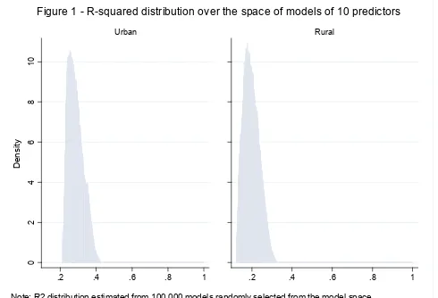
Figure 1 shows the R2 distribution over the space of 10-predictor models for urban and rural areas.
The distribution of R2 across the model space shows why targeting using PMT has inherent errors:
99.9% of models (of 10 predictors) predict less than 42% of the variation in actual household per
capita expenditures in urban areas, and less than 33% in rural areas.24 Model performance varies
widely between urban and rural areas. In urban areas, on average models of 10 predictors have an R2
of 0.29, whereas in rural areas the average R2 of 10-predictor models is about 0.20. It suggests that it
might be easier to identify poor households in urban areas than in rural areas based on the prediction
of their per capita expenditures using observable characteristics. This is possibly explained by
households tending to share similar socioeconomic characteristics in rural areas more than in urban
23
Robustness checks are conducted without the forcing of household size. The results for the ranking of the remaining predictors, available upon request, are the same.
24
16 areas, which makes the distinction between poor and non-poor households based on observables more
complex.25
4.2 The best predictors of household welfare
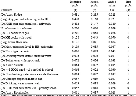
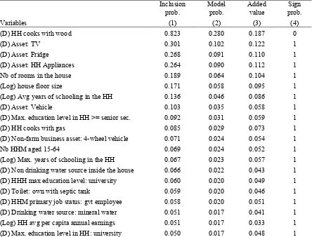
Tables 1a and 1b show the list of predictors that have a probability greater than 0.05 to be included in
the top 0.1% models and that have a consistent sign probability, ranked in descending order of their
inclusion probability, in urban and rural areas respectively.26 Variable inclusion probabilities in the
top 0.1% models are reported in column (1); the conditional probabilities to obtain a model which
performance classifies it among the top 0.1% when a given variable is included - referred to
henceforth as model probability - are reported in column (2). Variable added values, expressed as the
average share of added value in model R2, and their coefficient sign probabilities are reported in
columns (3) and (4) respectively. They are both conditional on each variable being included in a top
0.1% model. Tables 1a and 1b show that there is a high correlation between variable inclusion or
model probability and their added values.
The best predictors of welfare appear to belong to different variable categories, spanning from
education and employment to housing and asset ownership.27 In urban areas, the first three variables
25
Another reason for the lower predictive performance of rural models might be the fact that the poorest households are located in rural areas, whereas PMT does not allow targeting accurately enough the poorest of the poor. This stems from Ordinary Least Squares (OLS)-based predictions being inaccurate at the bottom of the consumption distribution (Grosh and Baker 1995).
26
See Annex 1.1 for the full list of variables, and a similar assessment of their performance in the top 0.1% models.
27
Variable categories that are not among the best predictors of welfare include variables that are less easy to collect and verify such as demographic dynamics, health status and nutrition.
0
Note: R2 distribution estimated from 100,000 models randomly selected from the model space.
17 appear significantly better than all other variables: they have a probability higher than 40% to be
included in a top 0.1% model. In such models, these variables contribute on average to increasing the
R2 by more than 12%. In rural areas, one variable, cooking with wood, is significantly better than all
other variables: more than 80% of the top 0.1% models include this variable. Furthermore, cooking
with wood contributes to nearly one-fifth of the R2 of these best models. This corresponds to an
increase of about 6 percentage points in the R2 of the top 0.1% rural models. Interestingly, it is also
the only variable among the best predictors that has a negative correlation with household welfare.28
Table 1a: Best predictors for the top 0.1% urban models
Inclusion
(D) Drinking water source: mineral water 0.076 0.026 0.037 1
(D) Toilet: own with septic tank 0.072 0.024 0.033 1
Note: HH stands for household, HHH for household head and HHM for household member; >=1 stands for at least 1. (D) indicates dummy variables. In all random models, the dependent variable is household adjusted per capita expenditures, and household size is included. The sign probabilities (probability that the variable has a positive sign) and added values (average difference between the squared of the 10-variable model - including the variable of interest - and the R-squared of the 9-variable model - excluding the variable of interest - as a share of the average R-R-squared of the top 0.1% 10-predictor models) are conditional on the variable being included. The model probability is the probability that the model is among the top 0.1% models, conditional on including a given variable.
28
18
Table 1b: Best predictors for the top 0.1% rural models
Inclusion
(D) Non-farm business asset: 4-wheel vehicle 0.071 0.024 0.054 1
Nb HHM aged 15-64 0.069 0.024 0.052 1
(D) Drinking water source: mineral water 0.051 0.017 0.041 1
(Log) HH avg per capita annual earnings 0.051 0.017 0.033 1
(D) Max. education level in HH: university 0.050 0.017 0.048 1
Note: HH stands for household, HHH for household head and HHM for household member; >=1 stands for at least 1. (D) indicates dummy variables. In all random models, the dependent variable is household adjusted per capita expenditures, and household size is included. The sign probabilities (probability that the variable has a positive sign) and added values (average difference between the squared of the 10-variable model - including the variable of interest - and the R-squared of the 9-variable model - excluding the variable of interest - as a share of the average R-R-squared of the top 0.1% 10-predictor models) are conditional on the variable being included. The model probability is the probability that the model is among the top 0.1% models, conditional on including a given variable.
Similarly to the R2 distribution, there appears to be best predictors that are specific to urban areas, and
others specific to rural areas, in addition to some variables that overlap between the two areas. This
suggests that obtaining good predictions of household welfare in Indonesia requires estimating PMT
formulas separately for urban and rural areas at least.29 The predictors that appear only in the top 0.1%
rural models are variables that allow distinguishing households whose living is not exclusively
dependent on farming and agriculture and that have diversified income sources (e.g. ownership of
non-farm business assets, being a government employee, the number of working-aged household
members). In addition, in rural areas ownership of private assets such as a TV or other appliances,
29
19 which could be categorized as non-vital or “convenience” assets, appear to contribute largely to
distinguish households by their welfare status.
In urban areas, are among the best predictors of welfare variables that are closely related to the
location of the dwelling, such as the type of floor, garbage disposal in a trash can or drinking water
from a well. These variables are likely to be correlated with dwellings located in slums, or
disadvantaged neighborhoods within cities; they describe the inequality in access to basic services and
sanitation, as well as the use of low quality construction material. Other predictors that are specific to
urban areas relate to the education participation of household members aged 15 and above, as well as
ownership of financial assets.
Robustness checks are conducted to assess whether the variable rankings obtained are sensitive to the
number of predictors selected in the random models or to the number of models estimated in the first
and second steps of the method. The results in terms of predictor ranking, available upon request, are
not affected by such changes in the implementation of the method. The model random sampling
method provides a ranking for all predictors in terms of their probability of being included in the top
performing models and their performance in explaining the variation in consumption or poverty (see
Appendix). The identification of good predictors of welfare is the first step in the estimation of a PMT
formula (PMTF). The second step relates to how to combine them in a PMTF, with practical
considerations such as the number of predictors to include. The next section discusses the predictive
performance of PMTFs using the good predictors of welfare.
Section 5 – The performance of proxy-means test formulas using the best predictors
Identifying the number of variables to include in the final PMTF involves a trade-off between (i) the
completeness of information, in order to explain as much of the variation in consumption or poverty
as possible, and (ii) the restriction of the number of variables, to limit the costs of collecting accurate
data. Furthermore, formulas with a high number of predictors are more subject to being not as valid
over-20 fitting problem. In this section, I compare PMTFs with 10, 20 and 30 of the best predictors of welfare,
in terms of their fit, as well as prediction errors and targeting incidence, to illustrate that this tradeoff
between completeness of information and model parsimony is not always in favor of the first.
5.1 Model fit
Figure 2 shows the observed increase in R2 and adjusted R2 obtained when increasing the number of
predictors one-by-one, in descending order of their inclusion probability in the top 0.1% 10-predictor
models. In urban areas the R2 reaches 0.50 with only 6 predictors. In rural areas, an R2 of 0.39 is
obtained with 10 predictors, and increasing the number of predictors to 40 yields an R2 higher by less
than 10 percentage points, at about 0.47. This shows that the marginal returns of adding more
predictors decreases in both areas, especially after about 10 predictors.
The difference between the R2 and the adjusted R2 of models of all sizes is hardly distinguishable,
including with 40 predictors. This suggests that even using the adjusted R2 as selection criterion leads
to selecting models with a large number of variables. Based on Figure 2, models of 40 predictors (or
more) should be selected in both areas as they have the highest adjusted R2.
.2
.4
.6
.5
.3
R
-s
q
ua
red
0 10 20 30 40
Number of predictors included Urban
0 10 20 30 40
Number of predictors included Rural
Figure 2 - Evolution of the R-squared with increases in the number of predictors
21
5.2 Model prediction errors
In this section, I assess whether gains in terms of fit from increasing the number of predictors also
leads to lower prediction errors, both in and out of sample. Prediction errors are measured by Type I
errors, or undercoverage, and Type II errors, or leakage rates. Undercoverage refers to households that
are in the target population based on their actual welfare, but are predicted to be above the eligibility
cutoff. Leakage refers to households wrongly predicted to have a welfare level that is below the
program eligibility cutoff whereas their actual welfare is above this cutoff. I use the predicted 30th
percentile as eligibility cutoff, which amounts to comparing the actual and predicted expenditure
deciles.30 I also calculate the severe undercoverage and severe leakage rates. The former refers to
households whose expenditures classify them in the first actual expenditures decile but that are
predicted to be above the 30th percentile eligibility cutoff point; the latter refers to households that are
predicted in the first expenditure decile whereas their actual expenditures classify them above the 30th
percentile.
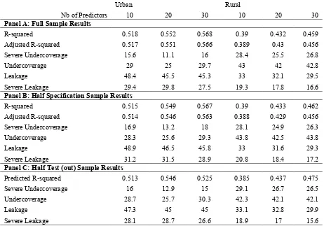
In-sample prediction errors of models with 10, 20 and 30 predictors are shown in Panel A of Table 2.
Undercoverage and severe undercoverage appear lower in urban areas, across all models. Models of
20 predictors are performing best in terms of undercoverage and severe undercoverage, in both areas.
About 11% of the poorest 10% are predicted above the 30th percentile with a 20-predictor model in
urban areas. Leakage and severe leakage rates appear marginally lower with 30-predictor models,
especially in rural areas.
In addition to full sample predictions, and in order to reduce the risk of selecting a model that overfits
the data, cross-validation tests are conducted. Models are estimated using one half of the sample –
estimation or specification sample - and the formulas generated are used to estimate predicted
consumption in the other half of the sample – test sample.31 This procedure allows mimicking the
30
Using the predicted 30th expenditure percentile as eligibility cutoff, which is the practice adopted in Indonesia, shifts the focus on household relative position within the distribution as predicted by the PMTF. This has the main advantage to allow offsetting the errors inherent to OLS predictions, which, by shrinking the consumption distribution, tend to predict higher expenditures for the poorest households. In addition, it allows better planning for programs, since it ensures that the number of households identified as eligible is closer to the expected coverage, in this case the poorest 30%.
31
22 real-world situation where PMT models are estimated using a consumption survey and applied to
calculate the predicted consumption of households surveyed in the targeting survey. The
cross-validation procedure also provides a test of the stability of the models when estimated with a smaller
sample. The prediction results for the specification and test samples are shown in Panels B and C of
Table 2. All models produce similar results in terms of R2 and prediction error rates, both with a
smaller estimation sample and out-of-sample. However, the performance of the urban model with 30
predictors can appear slightly less robust, since the predicted R2 out of sample is 4 percentage points
lower than the R2 obtained with the full and half specification samples, and the difference in severe
undercoverage and leakage rates is also slightly higher than for other models.
Table 2: Prediction accuracy of urban and rural models of different sizes - full and cross-validation samples.
Urban Rural
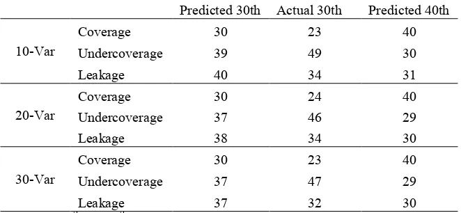
23 Table 3 presents the national level targeting prediction results, based on the estimation of urban and
rural models of different sizes. Undercoverage and leakage are based on two cutoffs, the actual and
the predicted 30th expenditure percentiles.32 When using the actual 30th percentile as eligibility cutoff,
the coverage is lower, about 23%, which leads to higher undercoverage and lower leakage compared
to the predicted 30th percentile. Table 3 shows that combined errors rates from models of 20 and 30
predictors are very similar, and at the 40th percentile all 3 models produce similar error rates.
Table 3: Overall prediction errors at different cutoff points.
Predicted 30th Actual 30th Predicted 40th
10-Var
Note: the 30th and 40th predicted eligibility cutoffs compare households in the actual and predicted expenditure deciles, while the actual 30th percentile eligibility cutoff
focuses on households whose predicted consumption is below the actual 30th consumption percentile.
5.3 Targeting incidence
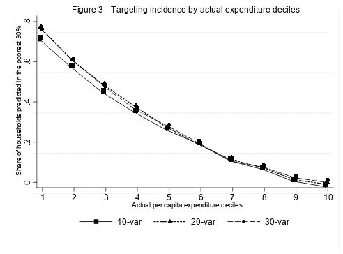
Lastly, I consider the combined targeting incidence and the distribution of predictions errors of urban
and rural models of 10, 20 and 30 predictors. Targeting incidence refers to the share of households in
each decile of the actual expenditure distribution that are predicted to be below the eligibility cutoff.
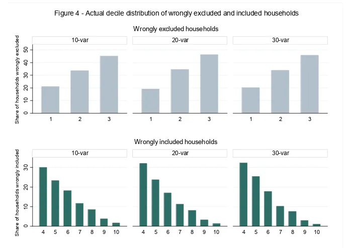
The distribution of prediction errors focuses on how households mis-predicted to be eligible or
non-eligible are distributed across actual consumption deciles. The idea is indeed that undercoverage is
less of a serious problem if households falsely excluded are close to the cutoff as opposed to at the
very bottom of the distribution; similarly, leakage is less grave if it includes households that are just
above the cutoff compared to households that are at the highest end of the distribution.
32
24 Even though deriving PMTFs induces rather significant errors in identifying the poor, targeting
appears highly progressive, and households that are wrongly excluded or included largely tend to be
classified in deciles that are relatively close to the eligibility cutoff, for all models. Figure 333 shows
that with all models the share of households predicted below the 30th percentile decreases rapidly
when going up in the deciles. The main gain in terms of increases in the share of poor households that
are identified as beneficiaries appears when going from 10 predictors to 20 predictors, although it is a
relatively small gain. The 30-predictor models perform similarly to the 10- and 20-predictor models
overall, except for the shares of households from the higher deciles, which are slightly lower with the
30-predictor models. Figure 4 shows that with all models more than 40% of households that are
wrongly predicted to be above the eligibility cutoff are actually in the third decile, and more than 50%
of households that are wrongly predicted to be below the predicted 30th expenditure percentile are
actually in the fourth and fifth deciles. Figure 4 also confirms that models of 20 predictors exclude
slightly fewer households from the first decile, whereas models of 30 predictors perform slightly
better in terms of inclusion errors, which concern more households from the fourth and fifth deciles.
Using 10, 20 or 30 predictors appears to produce relatively similar overall predictive performance. In
other words, models of 30 predictors are not significantly better, especially in terms of prediction
errors and targeting incidence. Based on the findings of this section, using models with 20 predictors
therefore seems a good trade-off between prediction accuracy and model parsimony. This is in line
33
When disaggregating the targeting incidence and the distribution of inclusion and exclusion errors from urban and rural models, a trend similar to that observed in Figures 3 and 4 is obtained, although, as discussed previously, urban models produce better predictions.
25 with Grosh and Baker (1995), who highlight that increasing the number of predictors has diminishing
returns in terms of the probability of collecting inaccurate information and thus the costs of
verification. With 2 models, one for urban and one for rural areas, using 20 predictors implies to
collect information on 28 indicators overall, which appears reasonable.
Section 6 – Recommendations and concluding remarks
Leamer (2010) advises that “it would be much healthier for all of us [economists] is we could accept
our fate, recognize that perfect knowledge will be forever beyond our reach and find happiness with
what we have.” In this chapter, it is acknowledged that it is impossible to find the best model to
predict household welfare. Instead, I propose a new method for selecting the predictors to use in PMT
formulas, based on the estimation of the distribution of predictive performance across the model space
and on the assessment of the sensitivity of the contribution of each candidate variable to model
performance.
I focus here on the recommendations based on the findings for Indonesia, where a PMT approach has
been used for identifying beneficiaries of social protection programs since 2005. Most recently, in
0
26 2011, the newly established Unified Database for Social Protection Programs34 (UDB) is also based
on PMT. As mentioned earlier, PMTF specific to each of the 497 Indonesian districts were developed
using the national socioeconomic survey, SUSENAS, and applied to data collected using the targeting
survey, 2011 Data Collection for Social Protection Programs (Pendataan Program Perlindungan
Social - PPLS). The findings of this paper provide useful recommendations for the updating of the
UDB, planned for 2014.
The correlates identified using the IFLS data confirm the multidimensional aspect of welfare and
poverty: the predictors shown to be robust predictors for welfare belong to different variable
categories, spanning from education and employment to housing and asset ownership. Most of these
variables are included in both the SUSENAS and PPLS. The first recommendation is therefore to add
the few good predictors that are not yet included in the Susenas and PPLS questionnaires, such as the
number of rooms in the house, the garbage being disposed of in a trash can and the distinction
between private and business assets. Moreover, the emphasis should be put on ensuring that the data
collected is of good quality. This is particularly important for the variables with the highest added
values in predicting households’ socioeconomic status. For collecting data on household size and on
other demographic indicators such as the number of members aged between 15 and 64, it is thus
recommended to use as much as possible official documents when they are available to the
respondents to complete the questionnaires. For other critical variables, in the education level,
housing and access to energy services categories in particular, enumerators have to be carefully
trained to collect quality information on these variables.
A combination of manual specification searches and stepwise procedure was used to select the
indicators that entered the 497 PMTF developed for the UDB. The method proposed in this paper can
be used as an alternative to identify – for each district or at a higher geographical level – good
predictors to be used for the updating of the PMTF in 2014. The implementation procedure adopted
here can be relatively easily automated using standard statistical softwares. Further, the robustness
34
27 checks carried out show that the ranking of predictors is consistent, including with the estimation of a
lower number of random models.
Regarding the predictive performance of the PMTFs, the results obtained in this paper are not directly
comparable with the models that have been developed for ranking households in the UDB, since they
were estimated using the SUSENAS instead of the IFLS, and since a model was developed for each
district. However, the average performance and size of these district-specific PMTF can be compared
for illustrative purposes with the ones developed here. On average, the district PMT formulas
currently used in Indonesia have 32 variables and are based on consumption regression models that
have an R-squared of 0.5. These models have predicted undercoverage and leakage rates at the
predicted 40th percentile cutoff of about 30%. The 10-, 20- and 30-predictor urban and rural models
developed in this paper have been shown to lead to similar prediction error rates. According to World
Bank (2012), there are significant gains in terms of targeting accuracy in estimating PMT formulas at
greater levels of geographical disaggregation, with the greatest gain obtained when going from
provincial- to district-level models. This suggests that using the model random sampling approach to
identify the best predictors of welfare could potentially allow both using a lower number of predictors
28
References
Ahmed A., and H. Bouis (2002): “Weighing What’s Practical: Proxy-Means Tests for Targeting Food Subsidies in Egypt”, Food Policy, 27: 519-540.
Castaneda T., and K. Lindert (2005): “Designing and Implementing Household Targeting Systems: Lessons from Latin America and the United States”, Social Protection Discussion Paper Series No. 0526”, Washington DC: The World Bank.
Coady D., Grosh M., and J. Hoddinott (2004): Targeting of Transfers in Developing Countries:
Review of Lessons and Experience, Washington D.C.: The World Bank.
Derksen S., and H. J. Keselman (1992): “Backward, Forward and Stepwise Automated Subset Selection Algorithms: Frequency of Obtaining Authentic and Noise Variables”, British Journal of Mathematical and Statistical Psychology, 45(2): 265–282.
Elbers C., Lanjouw J. O. and P. Lanjouw (2003): “Micro-Level Estimation of Poverty and Inequality,” Econometrica, 71(1): 355-364.
Glewwe P. and Kanaan, O. (1989): “Targeting assistance to the poor using household survey data”, Policy Research Working Paper Series 225, Washington DC: The World Bank.
Granger C. W. J. and H. F. Uhlig (1990): “Reasonable Extreme-Bounds Analysis,” Journal of Econometrics, 44(1-2): 159-70.
Grosh M. (1994): Administering Targeted Social Programs in Latin America: From Platitudes to
Practice. Washington DC: The World Bank.
Grosh M., and J. Baker. (1995)” “Proxy Means Tests for Targeting Social Programs: Simulations and Speculation”, Working Paper No. 118, Living Standards Measurement Study, Washington DC: The World Bank.
James F. C., and C. E. McCulloch (1990): “Multivariate Analysis in Ecology and Systematics: Panacea or Pandora's Box?” Annual Review of Ecology, Evolution, and Systematics 21: 129-166.
Judd C. M., and G. H. McClelland (1989): Data Analysis: A Model Comparison Approach. San Diego, CA: Harcourt, Brace, Jovanovitch.
Leamer E. E. (1978): Specification Searches: Ad Hoc Inference with Non-experimental Data, New York: Wiley, 1978.
Leamer E. E. (1983): “Let's take the Con Out of Econometrics”, American Economic Review, 73(3): 31-43.
29 Leamer E. E. (2010): “Tantalus on the Road to Asymptopia,” Journal of Economic Perspectives, 24(2): 31-46.
Levine, R. and D. Renelt (1992). A Sensitivity Analysis of Cross-Country Growth Regressions,
American Economic Review, 82(4): 942-963.
Narayan A., and N. Yoshida. (2005): “Proxy Means Test for Targeting Welfare Benefits in Sri Lanka”, PREM Working Paper 33258, South Asia Region, Washington DC: The World Bank.
Pradhan M., Suryahadi A., Sumarto S., and L. Pritchett (2003): “Eating Like Which “Joneses?” An Iterative Solution to the Choice of a Poverty Line “Reference Group””. Review of Income and Wealth
47 (4): 473–487.
Raftery A. E. (1995): “Bayesian model Selection in Social Research,” Sociological Methodology, 25: 111-163.
Sala-i-Martin X. (1997): “I Just Ran Two Million Regressions”, American Economic Review, 87(2): 178-183.
Sala-i-Martin X., Doppelhofer G., and R. I. Miller (2004): “Determinants of Long-Term Growth: A Bayesian Averaging of Classical Estimates (BACE) Approach.” American Economic Review, 94(4): 813-835.
Sharif, I. (2009): “Building a Targeting System for Bangladesh based on Proxy Means Testing”, Social Protection Discussion Paper No. 0914, Washington DC: The World Bank.
Strauss J., Beegle K., Dwiyanto A., Herawati Y., Pattinasarany D., Satriawan E., Sikoki B., Sukamdi and F. Witoelar (2004): Indonesian Living Standards Before and After the Financial Crisis: Evidence
from the Indonesia Family Life Survey, Santa Monica, CA: RAND Corporation, 2004.
Strauss J., Witoelar F., Sikoki B. and A.M. Wattie (2009): “The Fourth Wave of the Indonesia Family Life Survey (IFLS4): Overview and Field Report”, RAND Labor and Population, April 2009. WR-675/1-NIA/NICHD.
Sumarto S., Suryadarma D. and A. Suryahadi (2007): “Predicting Consumption Poverty using Non-Consumption Indicators: Experiments using Indonesian Data,” Social Indicators Research, 81(3): 543-578.
Temple J. (2000): “Growth Regressions and What the Textbooks Don’t Tell You”, Bulletin of
Economic Research 52 (3): 181-205.
30
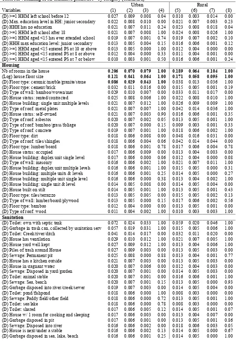
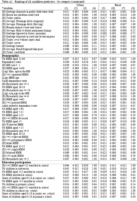
Appendix: Ranking of all candidate predictors – by category
31
Table A1 : Ranking of all candidate predictors - by category (continued)
Urban Rural
32
Table A1 : Ranking of all candidate predictors - by category (continued)
33
Table A1 : Ranking of all candidate predictors - by category (continued)
34
Table A1 : Ranking of all candidate predictors - by category (continued)
35
Table A1 : Ranking of all candidate predictors - by category (continued)
Urban Rural
Note: Results based on a random sample s2=1,000,000 models of 10 predictors. Columns (1) and (5): probabilities of being included in a
