Quadratic Nonnegative Matrix Factorization
Zhirong Yang∗, Erkki Oja
Aalto University, Department of Information and Computer Science, P.O.Box 15400, FI-00076, Aalto, Finland
Abstract
In Nonnegative Matrix Factorization (NMF), a nonnegative matrix is approx-imated by a product of lower-rank factorizing matrices. Most NMF methods assume that each factorizing matrix appears only once in the approximation, thus the approximation is linear in the factorizing matrices. We present a new class of approximative NMF methods, called Quadratic Nonnegative Matrix Factorization (QNMF), where some factorizing matrices occur twice in the approximation. We demonstrate QNMF solutions to four potential pattern recognition problems in graph partitioning, two-way clustering, estimating hidden Markov chains, and graph matching. We derive multiplicative algo-rithms that monotonically decrease the approximation error under a variety of measures. We also present extensions in which one of the factorizing ma-trices is constrained to be orthogonal or stochastic. Empirical studies show that for certain application scenarios, QNMF is more advantageous than other existing nonnegative matrix factorization methods.
Keywords: nonnegative matrix factorization, multiplicative update,
∗Corresponding author
Email addresses: [email protected](Zhirong Yang),[email protected]
stochasticity, orthogonality, clustering, graph partitioning, Hidden Markov Chain Model, graph matching
1. Introduction
Extensive research on Nonnegative Matrix Factorization (NMF) has emerged in recent years (e.g. [1, 2, 3, 4, 5, 6]). NMF has found a variety of applications in machine learning, signal processing, pattern recognition, data mining, in-formation retrieval, etc. (e.g. [7, 8, 9, 10, 11]). Given an input data matrix, NMF finds an approximation that is factorized into a product of lower-rank matrices, some of which are constrained to be nonnegative. The approxi-mation error can be measured by a variety of divergences between the input and its approximation (e.g. [12, 13, 14, 6]), and the factorization can take a number of different forms (e.g. [15, 16, 17]).
In most existing NMF methods, each factorizing matrix appears only once in the approximation. We call themlinear NMF because the approximation is linear with respect to each factorizing matrix. However, such linearity assumption does not hold in some important real-world problems. A typical example is graph matching, when it is presented as a matrix factorizing problem, as pointed out by Ding et al. [18]. If two graphs are represented by their adjacency matrices A and B, then they are isomorphic if and only if a permutation matrix P can be found such that A−PBPT = 0. Minimizing the norm or some other suitable error measure of the left-hand side with respect to P, with suitable constraints, reduces the problem to an NMF problem. The approximation is now quadratic in P.
to be clustered into r clusters, then the classical K-means objective function can be written as [19] J1 = T r(XTX)− T r(UTXTXU) where U is the
(n×r) binary cluster indicator matrix. The global minimum with respect to
U gives the optimal clustering. It was shown in [20] that minimizing J2 =
kXT − WWTXTk2
Frobenius with respect to an orthogonal and nonnegative
matrix W gives the same solution, except for the binary constraint. This is another NMF problem where the approximation is quadratic in W.
Although the need of quadratic factorizations has been occasionally ad-dressed in the literature (e.g. [21, 18, 17]), there has been no systematic study of higher-order NMF. A general way to obtain efficient optimization algorithms is lacking as well.
In this paper we focus on a class of NMF methods where some factor-izing matrices occur twice in the approximation. We call these methods
stochas-ticity or orthogonality constraint, needed for such applications as estimating a hidden Markov chain, clustering, or graph matching. (4) In addition to the advantages in clustering, already shown in our previous publication [20], we demonstrate that the proposed QNMF algorithms outperform the existing NMF implementations in graph partitioning, two-way clustering, estimating a hidden Markov chain, and graph matching.
In the rest of the paper, we first briefly review the nonnegative matrix factorization problem and related work in Section 2. Next we formulate the Quadratic Nonnegative Matrix Factorization problem in Section 3, with its multiplicative optimization algorithms, learning with the stochasticity and orthogonality constraints given in Section 4. Section 5 presents experimen-tal results, including comparisons between QNMF and other state-of-the-art NMF methods for four selected applications, as well as the demonstration of accelerated and online QNMF. Some conclusions and future perspectives are given in Section 6.
2. Related Work
Given an input data matrixX ∈Rm×n,Nonnegative Matrix Factorization
(NMF) finds an approximation Xb which can be factorized into a product of matrices:
X≈Xb =
Q
Y
q=1
F(q) (1)
and some of these matrices are constrained to be nonnegative. The dimen-sions of the factorizing matricesF(1), . . . ,F(Q)arem×r1, r1×r2, . . . , rQ−1×n,
the factorization represents the data in a more compact way and thus favors certain applications.
The difference between the input matrixX and its approximationXb can be measured by a variety of divergences, for which theoretically convergent multiplicative algorithms of NMF have been proposed1. Originally, NMF is
based on the Euclidean distance or I-divergence (non-normalized Kullback-Leibler divergence) [1, 2]. These two measures were later unified by using the
β-divergence [12]. Alternatively, Cichocki et al. [14] generalized NMF from I-divergence to the whole family of α-divergences. NMF has been further extended to a even broader class called Bregman divergence, for many cases of which a general convergence proof can be found [13]. In addition to separable ones, divergences that are non-separable with respect to the matrix entries such as theγ-divergence and R´enyi divergence can also be employed by NMF [11]. Many other divergences for measuring the approximation error in NMF exist, although they may lack theoretically convergent algorithms.
In its original form [1, 2], the NMF approximation is factorized into two matrices (Q = 2). Later the factorization was generalized to three factors (e.g. [23, 15, 16, 17]). Note that the input matrix and some factorizing matrices are not necessarily nonnegative, (e.g. Semi-NMF in [17]). Also, one of the factorizing matrix can be the input matrix itself, for example, the Convex NMF [17].
Besides the nonnegativity, various constraints or regularizations can be
1Unless otherwise stated, the term “convergence” in this paper generally refers to the
objective function convergence or, equivalently, the monotonic decrease of the NMF
imposed on the factorizing matrices. Matrix norms such as L1- or L2-norm
have been used for achieving sparseness or smoothness (e.g. [24, 3, 8]). Or-thogonality combined with nonnegativity can significantly enhance the part-based representation or category indication (e.g. [16, 25, 4, 26, 20]).
3. Quadratic Nonnegative Matrix Factorization
In most existing NMF approaches, the factorizing matrices F(q) in Eq. (1) are all different, and thus the approximation Xb as a function of them is linear. However, there are useful cases where some matrices appear more than once in the approximation. In this paper we consider the case that some of them may occur twice, or formally, F(s) = F(t)T for a number of non-overlapping pairs {s, t} and 1≤s < t≤Q. We call such a problem and its solution Quadratic Nonnegative Matrix Factorization (QNMF) because
b
X as a function is quadratic to each twice appearing factorizing matrix2.
To avoid notational clutter, we focus on the case where the input matrix and all factorizing matrices in the approximation are nonnegative, while our discussion can easily be extended to the cases where some matrices may contain negative entries by using the decomposition technique presented in [17].
3.1. Factorization forms
To begin with, let us consider the QNMF objective with only one doubly occurring matrix W. The general approximating factorization form is given
2Though equality without matrix transpose, namely F(s) = F(t), is also possible, to
by
b
X=AWBWTC, (2)
where we merge the products of the other, linearly appearing factorizing matrices into single symbols. It is also possible that matrix A, B, and/or C is the identity matrix and thus vanishes from the expansion. Here we focus on the optimization over W, as learning the matrices that occur only once can be solved by using the conventional NMF methods of alternative optimization over each matrix separately [11].
The above factorization form unifies all previously suggested QNMF ob-jectives. For example, it becomes the Projective Nonnegative Matrix Factor-ization (PNMF) when A = B = I and C = X, which was first introduced by Yuan and Oja [21] and later extended by Yang et al. [25, 27, 20]. This factorized form is also namedClustering NMF in [17] as a constrained case of
Convex NMF. Even without any explicit orthogonality constraint, the ma-trix W obtained by using PNMF is highly orthogonal and can thus serve two purposes: (1) when the columns ofXare samples, Wcan be seen as the basis for part-based representations, and (2) when the rows ofXare samples, W can be used as a cluster indicator matrix.
the learned W with the constraint WTW =I approximates a permutation matrix and thus QNMF can be used for learning order of relational data, for example, graph matching [18]. Alternatively, under the constraint that
W has column-wise unitary sums, the solution of such a QNMF problem provides parameter estimation of hidden Markov chains (See Section 5.3).
The factorization form in Eq. (2) also generalizes the concepts of Asym-metric Quadratic Nonnegative Matrix Factorization (AQNMF)Xb =WWTC and Symmetric Quadratic Nonnegative Matrix Factorization (SQNMF)Xb = WBWT in our previous work [22].
Note that the factorization form in Eq. (2) is completely general: it can be recursively applied to the cases where there are more than one factorizing matrices appearing quadratically in the approximation. For example, the case A=CT =U yields Xb =UWBWTUT, and A =B=I, C=XUUT yields Xb = WWTXUUT. An application of the latter example is shown in Section 5.2, where the solution of such a QNMF problem can be used to group the rows and columns ofX simultaneously. This is particularly useful for the biclustering or coclustering problem. These factorizing forms can be further generalized to any number of factorizing matrices. In such cases we employ alternative optimization over each doubly occurring matrix.
simul-taneously, which leads to higher-order objectives. For example, given the squared Frobenius norm (Euclidean distance) as approximation error mea-sure, the objective of linear NMF kX −WHk2
F is quadratic with respect
to W and H, whereas the PNMF objective kX−WWXk2
F is quartic with
respect toW. Minimizing such a fourth-order objective with the nonnegativ-ity constraint is considerably more challenging than minimizing a quadratic function.
In contrast to the rich selection of approximation error measures for lin-ear NMF, there is little reslin-earch on such measures for quadratic NMF. In this paper we show that QNMF can be built on a very wide class of dissimi-larity measures, quite as rich as those for linear NMF. Furthermore, as long as the QNMF objective can be expressed in a generalized polynomial form described below, we show that there always exists a multiplicative algorithm that theoretically guarantees convergence, or the monotonic decrease of the objective function, in each iteration.
In the rest of the paper, we distinguish the variable Wf from its current estimate W. We write Xe = AWBf WfTC to denote the approximation that contains the variable W, andf Xb = AWBWTC for the current estimate (constant).
3.2. Deriving multiplicative algorithms
maintain the nonnegativity of the factorizing matrices without any extra projection steps. Secondly, the fixed-point algorithm that iteratively applies the update rule requires no user-specified parameters such as the learning step size, which facilitates its implementation and applications. Although some heuristic connections to conventional additive update rules exist [2, 25], they cannot theoretically justify the objective function convergence.
The rigorous convergence proof, or theoretical guarantee of monotonic decrease of the objective function, focusses on minimizing a certain auxiliary upper-bounding function which is defined as follows. G(W,U) is called an auxiliary function if it is a tight upper bound of the objective functionJ(W), i.e. G(W,U)≥ J(W), and G(W,W) = J(W) for any W and U. Define
Wnew = arg min
f
W
G(Wf,W). (3)
By construction, J(W) = G(W,W) ≥ G(Wnew,W) ≥ G(Wnew,Wnew) =
J(Wnew), where the first inequality is the result of minimization and the
second comes from the upper bound. Iteratively applying the update rule (3) thus results in a monotonically decreasing sequence of J. Besides the tight upper bound, it is often desired that the minimization (3) has a closed-form solution. In particular, setting∂G/∂Wf = 0 should lead to the iterative update rule in analysis. The construction of such an auxiliary function, however, has not been a trivial task so far.
In [22], we recently derived the convergent multiplicative update rules for a wide class of divergences for the NMF problem. For conciseness, we repeat the central steps here but for details refer to [22].
vari-able z is of the form azb where a and b can take any real value, without
restriction to nonnegative integers. A sum of a (finite) number of monomials is called a (finite) generalized polynomial.
This form of expression has two nice properties: (1) individual mono-mials, denoted by azb, are either convex or concave with respect to z and
thus can easily be upper-bounded; (2) an exponential is multiplicatively de-composable, i.e. (xy)a=xaya, which is critical in deriving the multiplicative
update rule. Note that we unify the logarithm function that is involved in many information-theoretic divergences to our generalized polynomial form by using the logarithm limit
lnz = lim
ǫ→0+
zǫ−1
ǫ . (4)
Notice that limits in 0+ and 0− are the same. We use the former to remove
the convexity ambiguity. In this way, the logarithm can be decomposed into two monomials where the first contains an infinitesimally small positive exponent.
Next, we show that the auxiliary upper-bounding function always exists as long as the approximation objective function can be expressed in the finite generalized polynomial form. This is formalized by the following theorem in our previous work [22].
Theorem 1. Assume Ωd(z) = ρd·zχd, and ρd, χd, gdij andφd are constants
independent of Wf. If the approximation error has the form
then there are real numbers ψmax and ψmin (ψmax > ψmin) such that
and ∇− denote the sums of positive and unsigned negative terms of ∇ =
∂J(W)f
The theorem proof, or the construction procedure of the auxiliary function is summarized in the following procedure: 1) Write the objective function in the form of finite generalized polynomials given by Eq. (5); Use the logarithm limit Eq. (4) when necessary; 2) If the objective is not a separable sum over
i and j, i.e. there is χd 6= 1, derive a separable upper-bound of the objective
using the concavity or convexity inequality on Ωd; 3) Upper bound individual
monomials according to their concavity/convexity and leading signs; 4) If there are more than two upper-bounds with distinct exponents, combine them into two monomials according to their exponents and leading signs. The derivation details are similar to those given in our previous work [22] and thus omitted here.
Taking the derivative of the auxiliary function with respect to Wf leads to
In most cases, this multiplicative update rule has the form
In this case the limit of the derivative Eq. (7) has the form 00 and can be resolved by using the L’Hˆopital’s rule to obtain the limit before setting it to zero.
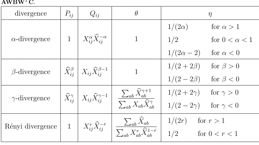
The finite generalized polynomial form Eq. (5) covers most commonly used dissimilarity measures. Here we present the multiplicative update rules for QNMF based on α-divergence, β-divergence,γ-divergence and R´enyi di-vergence. These families include, for example, the squared Euclidean distance (β = 1), Hellinger distance (α = 0.5), χ2-divergence (α = 2), I-divergence
(α → 1 or β → 0), dual I-divergence (α → 0), Itakura-Saito divergence (β → −1) and Kullback-Leibler divergence (γ → 0 or r → 1). Though not presented here, more QNMF objectives, for example the additive hybrids of the above divergences, as well as many other unnamed Csisz´ar divergences and Bregman divergences, can be easily derived using the proposed principle.
In general, the multiplicative update rules take the following form:
Table 1: Notations in the multiplicative update rules of QNMF examples, where Xb =
R´enyi divergence 1 Xr ijXbij−r
As an exception, the update rules for the dual I-divergence takes a different form
. In practice, iteratively applying the above update rules except the dual-I case can also achieve K.K.T. optimality asymptotically [22].
if the new objective is smaller than the old one and otherwise shrink back to the safe choice, η. We find that such a strategy can significantly speed up the convergence while still maintaining the monotonicity of the updates [22]. For very large data matrices, there are scalable implementations of QNMF for the case when the approximation error is the squared Euclidean distance. An online learning algorithm of PNMF was presented in our previous work [29], where we do not need to operate on the whole data matrix but only on a small intermediate variable instead. The resulting algorithm not only has low memory cost but runs faster than the batch version for large datasets.
4. Constrained QNMF
er-ror and forces the factorizing matrices to approach the constraint manifold. In what follows, we show how to get such a solution for QNMF with the stochasticity or orthogonality constraint.
4.1. Stochastic matrices
Nonnegative matrices are often used to represent probabilities, where all or a part of the matrix elements must sum up to one. For concreteness we only focus on the case of a left stochastic matrix with column-wise unitary sum, i.e. PiWik= 1, while the same method can easily be extended to
row-wise constraints (right stochastic matrix) or matrix-row-wise constraints (doubly stochastic matrix). A general principle that incorporates the stochasticity constraint to an existing convergent QNMF algorithm is given by the follow-ing theorem.
Theorem 2. Suppose a QNMF objective J(W)f to be minimized can be upper-bounded by the auxiliary function G(Wf,W) in the form of Eq. (6), whose gradient with respect to W is given in Eq. (7). Introducing a set of
Lagrangian multipliers {λk}, the augmented objective L(W,λ) = J(W) +f
P
kλk(1−PiWik) is non-increasing under the update rule
Wnew
ik =Wik
∇− ik+
P
a∇+akWak
∇+ik+Pa∇− akWak
σ
, (10)
where σ= 1/[max(ψmax,1)−min(ψmin,1)].
The proof is given in Appendix A. Note that the above reforming principle also includes the dual-I divergence case where max(ψmax,1)−min(ψmin,1) = 1
4.2. Orthogonal matrices
Orthogonality is another frequently used constraint in NMF [see e.g. 16, 18, 25, 4, 20] because a nonnegative orthogonal matrix has only one non-zero entry in each row. In this way the matrix can serve as a membership indicator in learning problems such as clustering or classification. Strict orthogonality is however of little interest in NMF because the optimization problem remains discrete and often NP-hard. Relaxation is therefore needed, as long as there is only one large non-zero entry in each row of the resulting W while the other entries are close to zero. An approximative orthogonal matrix is then obtained by simple thresholding and rescaling.
Here we present a general principle that incorporates the orthogonality constraint to a theoretically convergent QNMF algorithm. In Appendix we have proven the following results.
Theorem 3. Suppose a QNMF objective J(W)f to be minimized can be upper-bounded by the auxiliary function G(Wf,W) in the form of Eq. (6), whose gradient with respect to W is given in Eq. (7). Introducing a set of
Lagrangian multipliers {Λkl}, the augmented objective L(W,Λ) = J(W) +f
TrΛI−WfTWf is non-increasing under the update rule
Wnew
ik =Wik
"
∇−+WWT∇+
ik
(∇++WWT∇−) ik
#σ
, (11)
where σ= 1/[max(ψmax,2)−min(ψmin,0)].
Corollary 4. IfΛ+ = 12WT∇+ is positive semi-definite, thenσ= 1/[max(ψ
max,2)−
Our derivation of the multiplicative rules for learning nonnegative pro-jections is based on the Lagrangian approach. That is, one should apply WTW = I, one of the K.K.T. conditions, to simplify the resulting multi-plicative update rule after transforming Eq. (8) to its orthogonal counterpart Eq. (11). Furthermore, removing duplicate terms that appear in both nu-merator and denominator in practice will lead to faster convergent update rule because (a+c)/(b+c) is closer to one than a/b for a, b, c >0.
Although with highly orthogonal results, it is important to notice that W never exactly reaches the Stiefel or Grassmann manifold during the op-timization if it is initialized with positive entries. Therefore the reforming principle using natural gradients in such manifolds (e.g. [26, 4]) must be seen as an approximation.
5. Experiments
constraint for finding node correspondence of two graphs.
The following publicly available datasets have been used in our experi-ments: Newman’s collection3, the Pajek database4, the 3Conference graph5,
thewebkbtext dataset6, the top 58112 English words7, the GenBank database8,
and the University of Florida Sparse Matrix Collection9.
5.1. Graph partitioning
Given an undirected graph, the graph partitioning problem is to divide the graph vertices into several disjoint subsets, such that there are relatively few connections between the subsets. The optimization of many graph par-titioning objectives, for example, minimizing the number of removed edges in partitioning, is NP-hard due to the complexity of algorithms in a discrete space. It is therefore advantageous to employ a continuous approximation of the objectives, which enables the development of efficient gradient descent -type optimization algorithms by using differential calculus.
Suppose the connections in the graph are represented by a real-valued
N ×N affinity matrix A, whose element Aij gives the weight of the edge
connecting vertices i, j. A classical approximation approach is spectral clus-tering (e.g. [30]) which minimizes TrUT(D−A)U subject toUTDU=I, where Dis a diagonal matrix withDii=PjAij. Though the problem has a
3
http://www-personal.umich.edu/~mejn/netdata/
4http://vlado.fmf.uni-lj.si/pub/networks/data/
5http://users.ics.tkk.fi/rozyang/3conf/
6http://www.cs.cmu.edu/afs/cs.cmu.edu/project/theo-20/www/data/
7http://www.mieliestronk.com/wordlist.html
8http://www.ncbi.nlm.nih.gov/genbank/
closed form solution by using singular value decomposition, the resulting U may contain negative entries and thus cannot directly be used as an indicator for more than two clusters. An extra step that projects U to the positive quadrant is needed [31].
Ding et al. [18] presented the Nonnegative Spectral Clustering (NSC) method by introducing the nonnegativity constraint. They derived a mul-tiplicative update rule as an iterative Lagrangian solution that jointly min-imizes TrUT(D−A)U and forces U to approach the manifold specified by UTDU=I and U ≥0.
We can connect the NSC problem to the PNMF approach. Rewrit-ing W = D1/2U, which does not change the cluster indication because
D is diagonal and positive, the NSC problem becomes maximization of TrWT D−1/2AD−1/2W over nonnegativeWand subject toWTW=I.
This is a non-negative PCA problem which can be solved by PNMF [25, 20]. Furthermore, we can replaceD−1/2AD−1/2with some other symmetric
matri-ces or kernel matrimatri-ces. A good kernel can enhance the clustering effect of the graph and yield better partitioning results. Here we use a non-parametric ker-nel called random-walk kernel that minimizes the combinatorial formulation of the Dirichlet integral [32, 33, 34]. In brief, the kernel is obtained by sym-metrizing the solution of the following equation: (2D−A)B=A. Consider the reproducing Hilbert space induced by the kernelK= B+BT
2 whose entries
are nonnegative because B = (2D−A)−1A = 12D−1P∞ i=0
1
2AD
−1iA.
The graph partitioning problem can thus be solved by applying kernel PNMF [20] in the implicit feature space to minimizekΦ(X)T−WWTΦ(X)Tk2
F
ker-nel PNMF derived from the proposed principle isWnew We have compared the Nonnegative Spectral Clustering and our kernel
PNMF methods on four graphs: (1) Korea, a communication network of 39 women of two classes in Korea about family planning. (2) WorldCities, a dataset consists of the service values (indicating the importance of a city in the office network of a firm) of 100 global advanced producer service firms over 315 world cities. The firms are grouped into six categories: accountancy, advertising, banking/finance, law, insurance and management consultancy. (3) PolBlogs, a network of weblogs on US politics, with 1224 nodes. (4)
3Conference, the coauthorship network in three conferences SIGIR, ICML, and ICCV from 2002-2007. There are 2817 authors, 14048 edges in total. The value on each edge represents the number of papers that two authors have coauthored. The first three datasets are gathered from Newman’s collection3
and the Pajek database4. The3Conference graph is available at the authors’
website5.
We have computed the purities of the resulting partitions by using the ground truth class information: given r partitions and q classes, purity =
1
N
Pr
k=1max1≤l≤qNkl, where Nkl is the number of vertices in the partition k
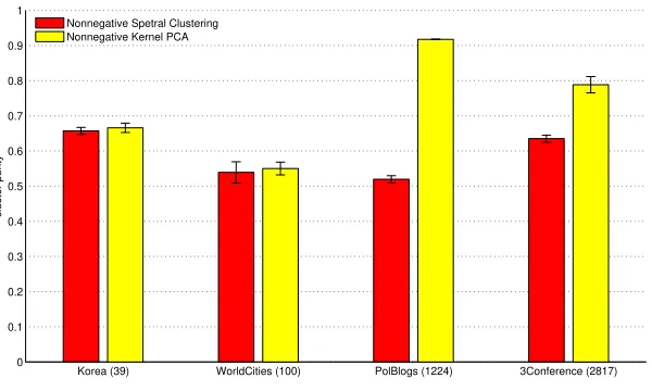
that belong to ground-truth classl. A larger purity in general corresponds to better clustering result. For each dataset, we repeated the compared methods 100 times with different random initializations and recorded the purities, whose means and standard deviations are illustrated in Figure 1. For small graphs Korea and WorldCities, kernel PNMF is at the same level or slightly better than the Nonnegative Spectral Clustering method. For larger graphs
Korea (39) WorldCities (100) PolBlogs (1224) 3Conference (2817) 0
0.1 0.2 0.3 0.4 0.5 0.6 0.7 0.8 0.9 1
cluster purity
Nonnegative Spetral Clustering Nonnegative Kernel PCA
Figure 1: Cluster purities using the two compared graph partitioning methods. Numbers
of graph nodes are shown in parentheses.
higher clustering purities.
The computational cost of both NSC and kernel PNMF is O(N2r) per
iteration. We have performed the above experiments using Matlab R2010b software on a personal computer with Intel Core i7 CPU, 8G memory and Ubuntu 10 operating system. For small graphs such asKorea and WorldCi-ties, the algorithms converged within a few seconds. For larger graphs such as PolBlogs and 3Conference, they converged within ten to fifteen minutes.
5.2. Two-way clustering
generate a blockwise visualization of the matrix when the rows and columns are ordered by their bicluster indices.
Two-way clustering has previously been addressed by the linear NMF methods (e.g. [8]). Given the factorization of the input matrix X ≈ WH, the bicluster index for each row of X is determined by the index of maximal entry in each row of W. The bicluster index for columns are likewise ob-tained. The biclustering problem has also been attacked by three-factor linear NMF X ≈ LSRT with the orthogonality constraint on L and R. For tri-factorizations, Ding et al. [16] gave a multiplicative algorithm called BiOR-NM3F when the approximation error is measured by the squared Euclidean distance. However, when this method is extended to other divergences such as the I-divergence, it is often stuck in trivial local minima where S tends to be smooth or even uniform because of the sparsity of L and R [15]. An extra constraint on S is therefore needed.
Here we propose to use a QNMF formulation for the biclustering problem:
X ≈ LLTXRRT. Compared with the BiOR-NM3F approximation, here we constrain the middle factorizing matrix S to be LTXR. The resulting two-sided QNMF objectives can be optimized by alternating the one-sided algorithms, that is, interleaving optimizations ofX ≈LLTY(R) withY(R)=
XRRT fixed and X ≈ Y(L)RRT with Y(L) = LLTX fixed. The bicluster indices of rows and columns are given by taking the maximum of each row in L and R. We call the new method Biclustering QNMF (Bi-QNMF) or
Two-way QNMF.
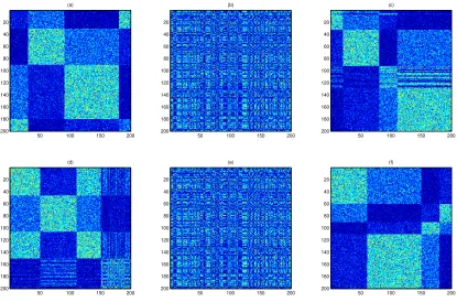
(a)
Figure 2: Biclustering usingα-NMF andα-PNMF based on the I-divergence for the
syn-thetic data: (a) the original matrix, (b) the disordered or testing matrix. The biclustering
results use (c) two-factor linear NMF, (d) BiOR-NM3F, (e) BiOR-NM3F-I and (f)
Bi-QNMF.
data. To our knowledge, BiOR-NM3F is implemented only for the squared Euclidean distance. For comparison, we apply the same development proce-dure by [16] (see also Section 4.2) to obtain the multiplicative update rules for the I-divergence, which we denote by BiOR-NM3F-I.
0 200 400 600 800
Figure 3: Biclustering using (from left to right) two-factor linear NMF, BiOR-NM3F,
BiOR-NM3F-I, and Bi-QNMF for thewebkb data.
from 1, 2, 4, or 7. The resulting generated matrix is visualized in Figure 2 (a) by using the Matlab command imagesc. The testing matrix is then obtained by randomly re-ordering the rows and columns of the original matrix. The biclustering task is to recover groups of rows and columns. With the learned factorizing matrices and corresponding bicluster indices, we reordered the rows and columns of the disordered matrix by ascending indices.
results in still disordered visualization. Compared to the above methods, Bi-QNMF can well reconstruct all biclusters up to a block-wise permutation. Next, we compared the four methods on the real-world webkb dataset6.
The data matrix contains a subset of the whole dataset, with two classes of 1433 documents and 933 terms. The ij-th entry of the matrix is the number of the j-th term that appears in the i-th document. Same as the tests on synthetic data, we reordered the matrix rows and columns by using the learned factorizing matrices of the compared methods. The resulting matrices are visualized in Figure 3 using the Matlab command spy.
The BiOR-NM3F method basically finds no biclusters. Only some small groups can barely be seen on the rightmost of the display. BiOR-NM3F-I is even worse, as there is no visually blockwise pattern in its result. The row cluster sizes found by the two-factor linear NMF and Bi-QNMF are roughly the same, about 650 rows for the first cluster and the rest for the second. However, linear NMF results in incoherent blocks, where the upper rows in the first row cluster are quite different from the others but very similar to the ones in the second row cluster. Such incoherence does not take place in the Bi-QNMF result, where the matrix is clearly divided into 2×2 biclusters.
Suppose the input matrix is of size m×n. The computational cost of BiOR-NM3F, BiOR-NM3F-I and Bi-QNMF is O(mn·max{rl, rr}) per
itera-tion, where rl andrr are number of columns ofL andR. For synthetic data,
5.3. Estimating hidden Markov chains
In a stationary Hidden Markov Chain Model (HMM), the observed out-put and the hidden state at time t are denoted by x(t) ∈ {1, . . . , n} and
y(t) ∈ {1, . . . , r}, respectively. The joint probabilities of a consecutive pair
are then given by Xij , P(x(t) = i, x(t + 1) = j) and Ykl , P(y(t) =
k, y(t+ 1) = l) accordingly. For the noiseless model, we haveX =WYWT with W , P(x(t) = i|y(t) = k). When noise is considered, this becomes an approximative QNMF problem X ≈ WYWT. Particularly, when the approximation error is measured by squared Euclidean distance, the pa-rameter estimation problem of HMM can be formulated as minimization of kX−WYWTk2
F over nonnegative W and Y and subject to
P
iWik = 1
for all k and PklYkl = 1.
Previously, the above optimization problem has been difficult because the objective is quartic with respect toW. An earlier algorithm, named NNMF-HMM [35], interleaves minimizations over Y and one of the appearances of W, each of which is implemented by using matrix pseudo-inversion and truncation of negative entries.
Now we have a much nicer algorithm for this QNMF problem. Using the presented deriving principle, we can obtain the multiplicative update rule in the form of Eq. (10), where ∇−
W = XWY
T + XTWY, ∇+
W =
WYWTWYT+WYTWTWY,∇−
Y =WTXW, and∇
+
Y =WTWYWTW.
10−2
Figure 4: Evolutions of the HMM estimation objective.
homo sapiens8. The sizes of the observed input matrix are 22×22, 26×26, and 64×64, respectively. We empirically set the number of hidden states in all experiments.
Both compared algorithms were run at least 10000 iterations. The evolu-tions of HMM estimation objective are shown in Figure 4. The new method is significantly more efficient than the old algorithm for all selected datasets. For the two smaller datasets, the objectives using NNMF-HMM tend to fluc-tuate a lot during the iterations, which is possibly caused by the brute-force truncation of negative entries. NNMF-HMM is more problematic for the largest dataset, where the approximation error only barely drops after thou-sands of epochs. By contrast, the objectives using QNMF-HMM decrease much faster and more stably.
QNMF-HMM uses soft constraints during its learning. To verify that the constraint errors are trivial in the converged results, we have checked the quantities Pk|1−PiWik| and |1−PklYkl| as constraint error measures
Table 2: Constraint errors using QNMF-HMM.
synthetic English words genetic codes
W 8.9e-06±3.8e-05 3.3e-05±3.5e-05 6.1e-06±6.1e-06 Y 1.7e-08±1.2e-07 2.2e-07±5.6e-07 2.7e-07±2.2e-07
synthetic English words genetic codes 10−5
10−4 10−3 10−2 10−1 100
converged objective (log−scale)
NNMF−HMM QNMF−HMM
Figure 5: HMM estimation objectives for the selected datasets.
deviations of the above constraint errors are shown in Table 2. We can see that the constraint errors are so small that they are negligible compared to the data dimensions.
We also examined the final objectives using the compared methods. For QNMF-HMM, we normalized W in the end of learning to force the strict constraints. The normalization actually causes little loss because of the neg-ligible constraint errors. The error bars of the final objectives are illustrated in Figure 5, from which we can see that the new method can achieve much smaller approximation errors than the old one. In addition, the variations of QNMF-HMM results are very small, which indicates the our method is pretty robust.
The squared Euclidean distance in the HMM estimation can be replaced with the Kullback-Leibler divergence, which is a more canonical difference measure for probabilities. With such divergence we can reveal some inter-esting structure in the fitted model of the English words data. Here we only focus on the QNMF-HMM algorithm because there is no existing imple-mentation or straightforward extension of NNMF-HMM for Kullback-Leibler divergence.
The latent or blockwise structure of the joint probability matrix X is visualized in Figure 6 by reordering the rows and columns according to the letter clusters, where lighter dots correspond to larger values. Each English letter was assigned to one of six clusters according to largest entries in the learned W rows. In this way we can group the letters into the following six groups: (1)D,Q,R,S,X, (2)C,G, (3)B,F,H,J,K,L,M,P,T,V,W,
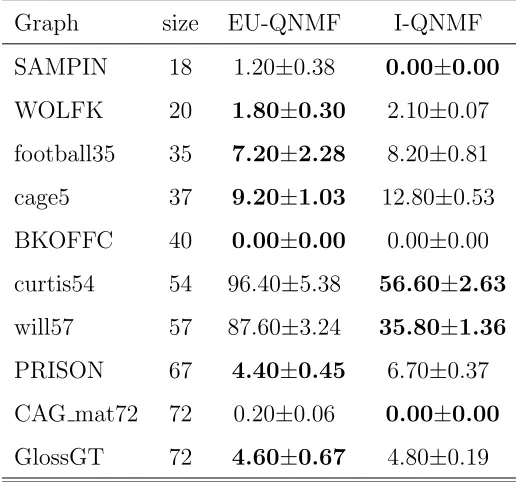
Table 3: Errors (mean±standard deviation) in directed graph matching.
Graph size EU-QNMF I-QNMF
SAMPIN 18 1.20±0.38 0.00±0.00 WOLFK 20 1.80±0.30 2.10±0.07 football35 35 7.20±2.28 8.20±0.81 cage5 37 9.20±1.03 12.80±0.53 BKOFFC 40 0.00±0.00 0.00±0.00 curtis54 54 96.40±5.38 56.60±2.63 will57 57 87.60±3.24 35.80±1.36 PRISON 67 4.40±0.45 6.70±0.37 CAG mat72 72 0.20±0.06 0.00±0.00 GlossGT 72 4.60±0.67 4.80±0.19
while the remaining two are basically vowels. A plausible interpretation of such division is that English words consist of syllables where a consonant is often followed by a vowel and vice versa. The letter N itself forms a group probably because we used a pretty large list of English words where suffixes such as ING and TION occur frequently.
5.4. Graph matching
The computation time of existing combinatorial algorithms to find the exact correct permutation grows exponentially as the number of nodes in-creases. For large graphs, approximation is therefore needed. A classical approximation algorithm by Umeyama [36] uses eigendecomposition and sim-ply forces nonnegativity by using absolute values of the eigenvectors. Ding et al. [18] pointed out that the results of Umeyama’s algorithm are not sat-isfactory, and proposed a special case of QNMF formulation based on the Euclidean distances: to minimizekB−WAWTk2
F subject toWTW=I and
W ≥ 0. After the multiplicative updates have converged, the permutation P is obtained by using the classical Hungarian algorithm on elementwise in-verse of WT [37]. This method, abbreviated by EU-QNMF, was reported to be superior to Umeyama’s algorithm on dense graphs generated as follows:
Aij = 100rij and Bij = (PtAPtT)ij(1 +ǫsij), where rij and sij are uniform
random numbers in [0, 1], Pt is a permutation and ǫ sets the noise level.
However, many real-world networks are not generated like this. They should be sparse and thus the Gaussian assumption that underlies the Euclidean-NMF does not hold. We are thus motivated to use the I-divergence, i.e. to minimize DI(B||WAWT) over W≥0 and subject to WTW=I. This
cor-responds to underlying Poisson distribution which is more suitable for sparse occurrences. We abbreviate the new method by I-QNMF.
The comparison results of EU-QNMF and I-QNMF for graph matching are shown in Tables 3 and 4 for directed and undirected graphs, respectively. All graphs in use are binary-valued. Most graphs were downloaded from the University of Florida Sparse Matrix Collection9. Some others were taken from
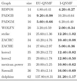
Table 4: Errors (mean±standard deviation) in undirected graph matching.
Graph size EU-QNMF I-QNMF
RDPOS 14 4.80±0.41 4.20±0.27 PADGB 16 9.20±0.98 10.20±0.64 PADGM 16 5.60±0.66 6.20±0.40 WOLFN 20 3.20±0.59 2.00±0.34 strike 24 25.60±1.36 12.20±1.02 ZACHC 34 43.20±4.76 10.40±0.08 ZACHE 34 27.60±2.97 5.00±0.36 korea1 35 39.20±2.72 12.40±0.82 korea2 35 29.60±1.78 12.80±0.50 mexican power 35 20.00±5.25 10.80±0.62 Sawmill 36 70.40±2.14 16.00±0.69 dolphins 62 137.80±8.31 31.20±1.17
comparison, we used a neutral quantity to measure the matching error, which is defined as #XOR(PAPT,B) , i.e. the number of different edges between
the estimated permuted matrix and the true permuted matrix. A smaller er-ror indicates better matching quality. In summary, I-QNMF performs almost at the same level as EU-QNMF for small or easy-matched graphs. However, the former is significantly better for larger and more difficult graphs in terms of both smaller mean errors and smaller deviations. This advantage is even clearer for undirected graphs.
The computational cost of both NMF graph matching algorithms isO(N3)
the algorithms can finish 20,000 iterations (converged) within a few seconds. For larger graphs such as GlossGT and dolphins, the algorithms converged within about ten minutes.
6. Conclusions
We have formulated the general problem of approximative quadratic non-negative matrix factorization and proposed a framework to develop multi-plicative optimization algorithms that are guaranteed to decrease the objec-tive function. Multiplicaobjec-tive algorithms for two typical QNMF factorization forms based on a great variety of approximation error measures, as well as the stochasticity and orthogonality constraints, were presented. The pro-posed method has been applied to four different pattern recognition problems, where QNMF is shown to be more advantageous than other state-of-the-art NMF methods.
algorithms for more divergence types other than squared Euclidean distance could be developed using advanced streaming or distributed computation techniques. Moreover, we have found that many QNMF multiplicative al-gorithms converge to similar local minima up to a certain component order. The theoretical analysis of the global minimum up to certain permutations needs further investigation.
Besides matrix products, the factorized approximation may involve non-linear operators, for example, a nonnon-linear activation function that interleaves a factorizing matrix and its transpose. This kind of approximation could be extended to the field of nonnegative neural networks and connected to the deep learning principle when multiple such groups of elements are stacked.
Appendix A. Proof of Theorem 2
Decompose λ into two nonnegative parts: λ = λ+−λ−, where λ+ bounds into two, we obtain the ultimate auxiliary function:
with σ = 1/(u− v). From ∂L(Wf,λ)/∂fWik = 0, we get (∇+ − ∇−)
Inserting this to Eq. (A.1), the multiplicative update rule becomes Eq. (10).
Appendix B. Proof of Theorem 3 and Corollary 4
Similar to the proof of Theorem 2, we decomposeΛinto two nonnegative parts: Λ = Λ+−Λ−. We can then construct the auxiliary function of the
The proof of Corollary 4 is similar to that of the theorem, except that we replace the bound of −Tr Λ+WTW with a hyper-plane −2PiklfWilΛ+lk+
constant. The corollary thus results in a larger exponential or step size σ
than Theorem 3.
References
[1] D. D. Lee, H. S. Seung, Learning the parts of objects by non-negative matrix factorization, Nature 401 (1999) 788–791.
[2] D. D. Lee, H. S. Seung, Algorithms for non-negative matrix factoriza-tion, Advances in Neural Information Processing Systems 13 (2001) 556– 562.
[3] P. O. Hoyer, Non-negative matrix factorization with sparseness con-straints, Journal of Machine Learning Research 5 (2004) 1457–1469.
[4] S. Choi, Algorithms for orthogonal nonnegative matrix factorization, in: Proceedings of IEEE International Joint Conference on Neural Net-works, 2008, pp. 1828–1832.
[5] D. Kim, S. Sra, I. S. Dhillon, Fast projection-based methods for the least squares nonnegative matrix approximation problem, Statistical Analysis and Data Mining 1 (1) (2008) 38–51.
[7] S. Behnke, Discovering hierarchical speech features using convolutional non-negative matrix factorization, in: Proceedings of IEEE Interna-tional Joint Conference on Neural Networks, Vol. 4, 2003, pp. 2758– 2763.
[8] H. Kim, H. Park, Sparse non-negative matrix factorizations via alternat-ing non-negativity-constrained least squares for microarray data analy-sis, Bioinformatics 23 (12) (2007) 1495–1502.
[9] A. Cichocki, R. Zdunek, Multilayer nonnegative matrix factorization using projected gradient approaches, International Journal of Neural Systems 17 (6) (2007) 431–446.
[10] C. Ding, T. Li, W. Peng, On the equivalence between non-negative matrix factorization and probabilistic latent semantic indexing, Com-putational Statistics and Data Analysis 52 (8) (2008) 3913–3927.
[11] A. Cichocki, R. Zdunek, A.-H. Phan, S. Amari, Nonnegative Matrix and Tensor Factorizations: Applications to Exploratory Multi-way Data Analysis, John Wiley, 2009.
[12] R. Kompass, A generalized divergence measure for nonnegative matrix factorization, Neural Computation 19 (3) (2006) 780–791.
[14] A. Cichocki, H. Lee, Y.-D. Kim, S. Choi, Non-negative matrix factor-ization with α-divergence, Pattern Recognition Letters 29 (2008) 1433– 1440.
[15] A. Pascual-Montano, J. M. Carazo, K. Kochi, D. Lehmann, R. D. Pascual-Marqui, Nonsmooth nonnegative matrix factorization (nsNMF), IEEE Transactions on Pattern Analysis and Machine Intelli-gence 28 (3) (2006) 403–415.
[16] C. Ding, T. Li, W. Peng, H. Park, Orthogonal nonnegative matrix t-factorizations for clustering, in: Proceedings of the 12th ACM SIGKDD international conference on Knowledge discovery and data mining, 2006, pp. 126–135.
[17] C. Ding, T. Li, M. I. Jordan, Convex and semi-nonnegative matrix fac-torizations, IEEE Transactions on Pattern Analysis and Machine Intel-ligence 32 (1) (2010) 45–55.
[18] C. Ding, T. Li, M. I. Jordan, Nonnegative matrix factorization for com-binatorial optimization: Spectral clustering, graph matching, and clique finding, in: Proceedings of the 8th IEEE International Conference on Data Mining (ICDM), 2008, pp. 183–192.
[19] C. Ding, X. He, K-means clustering via principal component analysis, in: Proceedings of International Conference on Machine Learning (ICML), 2004, pp. 225–232.
factorization, IEEE Transaction on Neural Networks 21 (5) (2010) 734– 749.
[21] Z. Yuan, E. Oja, Projective nonnegative matrix factorization for image compression and feature extraction, in: Proceedings of 14th Scandina-vian Conference on Image Analysis (SCIA), Joensuu, Finland, 2005, pp. 333–342.
[22] Z. Yang, E. Oja, Unified development of multiplicative algorithms for linear and quadratic nonnegative matrix factorization, IEEE Transac-tion on Neural NetworksAccepted, to appear.
[23] B. Long, Z. Zhang, P. S. Yu, Coclustering by block value decomposition, in: Proceedings of the eleventh ACM SIGKDD international conference on Knowledge discovery in data mining, 2005, pp. 635–640.
[24] W. Liu, N. Zheng, X. Lu, Non-negative matrix factorization for visual coding, in: Proceedings of IEEE International Conference on Acoustics, Speech, and Signal Processing (ICASSP), Vol. 3, 2003, pp. 293–296.
[25] Z. Yang, J. Laaksonen, Multiplicative updates for non-negative projec-tions, Neurocomputing 71 (1-3) (2007) 363–373.
[26] J. Yoo, S. Choi, Orthogonal nonnegative matrix factorization: Multi-plicative updates on Stiefel manifolds, in: Proceedings of the 9th In-ternational Conference on Intelligent Data Engineering and Automated Learning, 2008, pp. 140–147.
Journal on Pattern Recognition and Artificial Intelligence 21 (8) (2007) 1353–1362.
[28] E. M. Airoldi, D. M. Blei, S. E. Fienberg, E. P. Xing, Mixed membership stochastic blockmodels, Journal of Machine Learning Research 9 (2008) 1981–2014.
[29] Z. Yang, E. Oja, Online projective nonnegative matrix factorization for large datasets, in: NIPS Workshop on Low-rank Methods for Large-scale Machine Learning, 2010.
[30] J. Shi, J. Malik, Normalized cuts and image segmentation, IEEE Trans-actions on Pattern Analysis and Machine Intelligence 22 (8) (2000) 888– 905.
[31] S. X. Yu, J. Shi, Multiclass spectral clustering, in: Proceedings of the 9th IEEE International Conference on Computer Vision, Vol. 2, 2003, pp. 313–319.
[32] X. Zhu, Z. Ghahramani, J. Lafferty, Semi-supervised learning using gaussian fields and harmonic functions, in: Proceedings of the 20th In-ternational Conference on Machine Learning (ICML), 2003, pp. 912–919.
[33] L. Grady, Random walks for image segmentation, IEEE Transactions on Pattern Analysis and Machine Intelligence 28 (11) (2006) 1768–1783.
[35] B. Lakshminarayanan, R. Raich, Non-negative matrix factorization for parameter estimation in hidden markov models, in: Proceedings of IEEE International Workshop on Machine Learning For Signal Processing, 2010, pp. 89–94.
[36] S. Umeyama, An eigendecomposition approach to weighted graph matching problems, IEEE Transactions on Pattern Analysis and Ma-chine Intelligence 10 (5) (1988) 695–703.
[37] H. W. Kuhn, The Hungarian method for the assignment problem, Naval Research Logistics Quarterly 2 (1955) 83–97.
[38] C.-J. Lin, Projected gradient methods for non-negative matrix factor-ization, Neural Computation 19 (2007) 2756–2779.