arXiv:1711.06466v1 [q-fin.MF] 17 Nov 2017
David Hobson
∗and
Dominykas Norgilas
†Department of Statistics, University of Warwick
Coventry CV4 7AL, UK
November 20, 2017
Abstract
We consider the problem of finding a model-free upper bound on the price of an American put given the prices of a family of European puts on the same underlying asset. Specifically we assume that the American put must be exercised at either T1 orT2 and that we know the prices of all vanilla European puts with these maturities. In this setting we find a model which is consistent with European put prices and an associated exercise time, for which the price of the American put is maximal. Moreover we derive a cheapest superhedge. The model associated with the highest price of the American put is constructed from the left-curtain martingale transport of Beiglb¨ock and Juillet.
Keywords: Model-independent pricing, American put, Martingale Optimal Transport, Optimal stopping
Mathematics Subject Classification: 60G40, 60G42, 91G20
1
Introduction
This article is motivated by an attempt to understand the range of possible prices of an American put in a robust, or model-independent, framework. In out interpretation this means that we assume we are given today’s prices of a family of European-style vanilla puts (for a continuum of strikes and for a discrete set of maturities). The goal is to find the consistent model for the underlying for which the American put has the highest price, where by definition a model is consistent if the discounted price process is a martingale and if the model-based discounted expected values of European-put payoffs match the given prices of European puts.
This notion of model-independent or robust bounds on the prices for exotic options was introduced in Hobson [14] in the context of lookback options, and has been applied several times since, see Brown et al. [7] (barrier options), Cox and Ob l´oj [10] (no-touch options), Hobson and Klimmek [16] (forward-start straddles), Carr and Lee [8] and Cox and Wang [11] (variance options), Herrmann and Stebegg [13] (Asian options) and the survey article Hobson [15]. The principal idea is that the prices of the vanilla European puts determine the marginal distributions of the price process at the traded maturities (but not the joint distributions) and that these distributional requirements, coupled with the martingale property, place meaningful and useful restrictions on the class of consistent models. These restrictions lead to bounds on the expected payoffs of path-dependent functionals, or equivalently bounds on the prices of exotic options.
In addition to the pricing problem there is a related dual or hedging problem. In the dual problem the aim is to construct a static portfolio of European put options and a dynamic discrete-time hedge in the underlying which combine to form a superhedge (pathwise over a suitable class of candidate price paths) for the exotic option. The value of the dual problem is the cost of the cheapest superhedge.
There is a growing literature, beginning with Beiglb¨ock et al. [3], which aims to explain how to formulate the problem in such a way that there is no duality gap, i.e. the highest model-based price is equal to the cheapest superhedge, either for specific derivatives, or for a wide class of payoffs simultaneously.
Many of the early papers on robust hedging exploited a link with the Skorokhod embedding problem (Skorokhod [22]). For example, in the study of the lookback option in Hobson [14] the consistent model which achieves the highest lookback price is constructed from the Az´ema-Yor [1] solution of the Skorokhod embedding problem. More recently, Beiglb¨ock et al [3] have championed the connection between robust hedging problems and martingale optimal transport. In this paper we will make use of the left-curtain martingale transport of Beiglb¨ock and Juillet [4].
The study of American style claims in the robust framework was initiated by Neuberger [21], see also Hobson and Neuberger [19] and Bayraktar and Zhou [2]. (There is also a paper by Cox and Hoeggerl [9] which asks about the possible shapes of the price of an American put, considered as a function of strike, given the prices of co-maturing European puts.) The main innovation of this paper is that rather than focussing on general American payoffs and proving that the pricing (primal) problem and the dual (hedging) problem have the same value, we focus explicitly on American puts and try to say as much as possible about the structure of the consistent price process for which the model-based American put price is maximised, and the structure of the cheapest superhedge.
Mathematically, it will turn out that our problem can be cast as follows. Letµ and ν be a pair of probability measures which are increasing in convex order and therefore necessarily have the same mean ¯µ. A standing assumption in this paper will be thatµhas no atoms. Let ˆΠM(µ, ν) be the set of
martingale couplings betweenµand ν and letK1> K2be a pair of fixed constants. The problem we
consider is to find
Borel subset ofR. In terms of the American put problemM should be thought of as the discounted price of the underlying asset (to simplify notation we writeM1≡X andM2≡Y). Further, K1and
K2 are the discounted strikes of the put and B represents the set of values of the discounted time-1
price of the underlying such that the option is exercised at time-1; otherwise the put is exercised at time-2. Then (1) represents the primal problem of finding the highest model-based expected payoff of the American put. See Section 2.2.
There is a corresponding dual or hedging problem of finding a cheapest superhedge based on static portfolios of European puts and a piecewise constant holding of the underlying asset, see Section 2.3. Our main achievement isto exhibit the model and stopping rule which achieves the highest possible price for the American put, to exhibit the cheapest superhedge, and to show that the highest model-based price is equal to the cost of the cheapest superhedge.
For fixedµ, νandK1> K2there is typically a family of optimal models. Fixingµandνbut varying
K1 and K2 it turns out that there is a model which is optimal for allK1 and K2 simultaneously. If
µ is continuous, then this model is related to the left-curtain coupling of Beiglb¨ock and Juillet [4]. In particular, given µ ≤cx ν (with µ continuous), Beiglb¨ock and Juillet [4] prove that there exist
functionsTd and Tu withTd(x)≤x≤Tu(x) such thatTu is increasing and such that if x < x′ then
Td(x′)∈/ (Td(x), Tu(x)), and such that there isπ ∈ΠˆM(µ, ν) which is concentrated on the graphs of
Td and Tu. Under this martingale transport Y ∈ {Td(X), Tu(X)} and by the martingale property
P(Y =Td(X)|X) =TTu(X)−X
u(X)−Td(X) (assuming not bothTd(X) =X andTu(X) =X).
In this paper we will concentrate on the case whereµis continuous. Indeed, ifµhas atoms then the situation becomes more delicate. On one hand, we must allow for a wider range of possible candidates for exercise determining sets B. On atoms of X we may want to sometimes stop and sometimes continue, although we must still take stopping decisions which do not violate the martingale property of future price movements. On the other hand, the functionsTd,Tuthat characterises the left-curtain
model can be identified. For these reasons we must extend our notion of a martingale coupling and generalise, in a useful fashion, the left-curtain martingale coupling of [4] to the case with atoms. The appropriate extension of the left-curtain transport to the case with atoms in µ is discussed in a companion paper ([20]); in this paper we focus on the financial aspects of our results, namely the application to the robust hedging of American puts.
The remainder of the paper is structured as follows. In the next section we formulate precisely our problem of finding the robust, model-independent price of an American put and explain how the problem can be transformed into (1) in the atom-free case. We also explain how the pricing problem is related to the dual problem of constructing the cheapest superhedge. In Section 3 we assume that µis continuous, and we show by studying a series of ever more complicated set-ups how to determine the best model and hedge. The constructions in this section make use of the left-curtain mapping of Beiglb¨ock and Juillet [4].
By weak duality the highest model price is bounded above by the cost of the cheapest superhedge. Hence, if on the one hand we can identify a consistent model and stopping rule and on the other a superhedge, such that the expected payoff in that model with that stopping rule is equal to the cost of the superhedge then we must have identified an optimal model and an optimal stopping rule together with an optimal hedging strategy. Moreover there is no duality gap. This is the strategy of our proofs. One feature of our analysis is that wherever possible we provide pictorial explanations and derivations of our results, involving drawing well chosen tangents and other lines on various figures. In our view this approach helps bring insights which may be hidden from calculus-based approaches.
2
Preliminaries and set-up
2.1
Measures and Convex order
Given an integrable measureη (not necessarily a probability measure) onRdefine ¯η=
R
Rxη(dx)
R
Rη(dx) to be barycentre of η. LetIη with endpoints{ℓη, rη} be the smallest interval containing the support ofη.
DefinePη:R7→R+ byPη(k) =R k
−∞(k−x)η(dx). Then Pη is convex and increasing, and represents
the discounted European put-price, expressed as a function of strike, if the discounted underlying has lawη at maturity. Further,{k:Pη(k)> η(R)(k−η)¯ +} ⊆ Iη. Note thatPη is related to the potential
Uη defined byUη(k) :=−RR|k−x|η(dx) byPη(k) =12(−Uη(k) + (k−η)η(¯ R)).
Two measuresη andχare in convex order and we writeη≤cxχif and only ifη(R) =χ(R), ¯η= ¯χ
andPη(k)≤Pχ(k) on R. Necessarily we must haveℓχ ≤ℓη ≤rη ≤rχ. Let ˆΠM(η, χ) be the set of
martingale couplings ofη andχ. Then ˆ
ΠM(η, χ) =π∈ P(R2) :πhas first marginalη and second marginalχ; (2) holds
whereP(R2) is the set of probability measures onR2and (2) is the martingale condition
Z
The following lemma tells us that ifDη,χ(x) = 0 for somexthen in any martingale coupling ofη
andχ, no mass can crossx.
Lemma 1. Supposeη andχare probability measures with equal means and thatη≤cxχ.
Proof. If (¯η, X, Y) is a martingale withX ∼η andY ∼χthen
Pχ(x) =E[(x−Y)+]≥E[(x−Y)+;X≤x]≥E[(x−Y);X ≤x] =E[(x−X);X≤x] =Pη(x). (3)
IfD(x) = 0 we must have equality in the first two inequalities. From the fact that the first inequality is an equality we conclude that (Y < x) ⊆ (X ≤ x) and π((x,∞),(−∞, x)) = 0. Observe that (3) also holds if we replace (X ≤ x) with (X < x). Again, if D(x) = 0 there is equality in the first two inequalities. This time from the second inequality we conclude (Y > x) ⊆ (X < x)c and π((−∞, x),(x,∞)) = 0.
It follows from Lemma 1 that if there is a point x in the interior of the interval Iη such that
Dη,χ(x) = 0 then we can separate the problem of constructing martingale transports of η to χ into
a pair of subproblems involving mass to the left and right of x respectively, always taking care to allocate mass ofχ at xappropriately. Indeed, if there are multiple {xj} with Dη,χ(xj) = 0 then we
can divide the problem into a sequence of ‘irreducible’ problems, each taking place on an intervalIi
such thatD >0 on the interior ofIi andD= 0 at the endpoints. All mass starting in a given interval
is transported to a point in the same interval. However, in our setting, in addition to specifying a model (or equivalently a martingale transport) we also need to specify a stopping rule, and this needs to be defined across all irreducible components simultaneously. For this reason we do not insist that D >0 on the interior ofIχ, although this will be the case in the simple settings in which we build our
solution.
2.2
The financial model and model based prices for American puts
Suppose ˜Z = ( ˜ZTi)i=0,1,2is the price of a financial security which pays no dividends, whereT0= 0 is
today’s date. Suppose interest rates are non-stochastic and positive. Let one unit of cash invested in a bank account paying the riskless rate be worth ˜BTi at time ifor i= 0,1,2. Then ˜B0 = 1. Define
Z = (Zi)i=0,1,2 byZi= ˜ZTi/B˜Ti so thatZ is the discounted asset price with a simplified time-index
i= 0,1,2. We assume thatZ0 is known at time 0.
Let Σ be the set of stopping rules taking values in{T1, T2} and let T be the set of stopping rules
taking values in{1,2}. Consider an American put with strike Kwhich may be exercised at T1 orT2
only. Define Ki = K/B˜Ti. Under a fixed model the expected payoff of an American put under an
exercise (stopping) ruleσ taking values in{T1, T2} is given byE[B˜1σ(K−Z˜σ)+] and the price of the
American option (assuming exercise is only allowed atT1or T2) is
sup
the call prices have come from a model for which the discounted price process is a martingale then
˜
Henceforth we assume we work in a discounted setting and with time-index in the seti= 0,1,2. In this setting the American put has payoff (K1−Z1)+ at time 1 and payoff (K2−Z2)+ at time 2 where
European puts (with maturitiesT1andT2in the original timescale) for all possible strikes. From these
we can infer the laws of the discounted price process at times 1 and 2. We denote these laws byµand ν. It follows from Jensen’s inequality that ifµandν have arisen from sets of European put options in this way thenµ≤cxν.
Definition 1. Supposeµ≤cxν.
Let S = (Ω,F,P,F ={F0,F1,F2}) be a filtered probability space. We say M = (M0, M1, M2) =
(¯µ, X, Y) is a(S, µ, ν)consistent stochastic process and we write M ∈ M(S, µ, ν) if 1. M is aS-martingale
2. L(M1) =µandL(M2) =ν
We say (S, M) is a (µ, ν)-consistent model if S is a filtered probability space and M is a (S, µ, ν)
consistent stochastic process.
LetB ∈ F1. Define the stopping time τB by τB = 1 on B and τB = 2 on Bc. (Conversely, any
stopping rule taking values in {1,2} has a representation of this form.) Suppose (S,M) is a (µ, ν) consistent model. The (S, M) model-based expected payoff of the American put under stopping rule τB is
A(B, M,S) =E[(KτB−MτB)
+].
Then, optimising over stopping rules under the model (S, M) the price of the American put is
A(M,S) = supBA(B, M,S). The highest model based expected payoff for the American put is
P = sup
S
sup
M∈M(S,µ,ν)
sup
B
A(B, M,S). (4)
Remark 1. It is important to note that the supremum in (4)can exceed the supremum in (1), but only in the case whereµhas atoms. See Hobson and Norgilas [20]. The supremum in (1) gives the highest model based price under the restriction that F0 is trivial, F1 =σ(X) and F2 =σ(X, Y). However, as pointed out in Hobson and Neuberger [19], see also Hobson and Neuberger [18] and Bayraktar and Zhou [2], it is sometimes possible to achieve a higher model price if we work on a richer probability space. In the financial context, the choice of probability space is typically not specified. Instead the choice of probability space is a modelling issue, and it seems unreasonable to restrict attention to a sub-class of models without good reason, especially if this sub-class does not include the optimum.
2.3
Superhedging
The following notion of a robust superhedge for an American option was first introduced by Neu-berger [21], see also Bayraktar and Zhou [2] and Hobson and NeuNeu-berger [19].
We work in discounted units over two time-points. Consider a general American-style option with payoffaif exercised at time 1, and payoffbif exercised at time 2. We assumea≥b≥0.
Definition 2. (φ, ψ,{θi}i=1,2) is a superhedge for(a, b)if
a(x) ≤ φ(x) +ψ(y) +θ1(x)(y−x), (5)
b(y) ≤ φ(x) +ψ(y) +θ2(x)(y−x). (6) The cost of a superhedge is given by
C=C(φ, ψ,{θi}i=1,2;µ, ν) =
Z
φ(x)µ(dx) +
Z
ψ(y)ν(dy),
where we setC=∞if R
φ(x)+µ(dx) +R
The idea behind the definition is that the hedger purchases a portfolio of maturity-1 European puts (and calls) with payoffφand a portfolio of maturity-2 European puts (and calls) with payoffψ. (The fact that this can be done and has costC follows from arguments of Breeden and Litzenberger [6].) In addition, if the American option is exercised at time-1 the hedger holdsθ1units of the underlying
between times 1 and 2; otherwise the hedger holds θ2 units of the underlying over this time-period.
In the former case, (5) implies that the strategy superhedges the American option payout; in the later case (6) implies the same.
Remark 2. We could extend the definition and allow a holding of θ0 units of the discounted asset over the time-period[0,1). Then the RHS of (5) would be
φ(x) +ψ(y) +θ0(x−M0) +θ1(x)(y−x). (7) However, after a relabelling φ(x) +θ0(x−M0) 7→ φ(x), (7) reduces to (5). (Note that Rθ0(x−
M0)µ(dx) = 0 by the martingale property so thatC is unchanged.) Similarly for (6). Hence there is no gain in generality by allowing non-zero strategies between times 0 and 1.
The dual (superhedging) problem is to find
D(µ, ν;a, b) = inf
(φ,ψ,{θi}i=1,2)∈H(a,b)
C(φ, ψ,{θi}i=1,2;µ, ν). (8)
Potentially the space H could be very large and it is extremely useful to be able to search over a smaller space. The next lemma shows that any convex ψ with ψ ≥ b can be used to generate a superhedge (φ, ψ,{θi}i=1,2). Letχ′+ denote the right-derivative of the convex functionχ.
Lemma 2. Supposeψ≥b withψ convex. Defineφ= (a−ψ)+ and setθ
2= 0 andθ1=−ψ+′ . Then
(φ, ψ,{θi}i=1,2)is a superhedge. Proof. We have
b(y)≤ψ(y)≤φ(x) +ψ(y) =φ(x) +ψ(y) +θ2(x)(y−x)
and (6) follows. Also, by the convexity ofψ,ψ(x)≤ψ(y)−ψ′
+(x)(y−x) and
a(x)≤(a(x)−ψ(x))++ψ(x)≤φ(x) +ψ(y) +θ1(x)(y−x).
Hence (5) follows.
Let ˘H= ˘H(b) be the set of convex functionsψwithψ≥b. For ψ∈H˘ we can define the associated cost of the portfolio
˘
C(ψ;µ, ν) =
Z
(a(x)−ψ(x))+µ(dx) +Z ψ(y)ν(dy)
The reduced dual hedging problem restricts attention to superhedges generated fromψ∈H˘ and is to find
˘
D= ˘D(µ, ν;a, b) = inf
ψ∈H˘(b)
˘
C(ψ;a, b). (9)
Clearly we haveD ≤D˘: we will show thatD= ˘Dfor the American put.
2.4
Weak and Strong Duality
Let (S, M) be a (µ, ν) consistent model and letτbe a stopping time in this framework. The expected payoff of the American put under this stopping rule isE[(Kτ−Mτ)+]. Conversely, letψbe any convex
function withψ(y)≥(K2−y)+and letφ(x) = [(K1−x)+−ψ(x)]+ andθi(x) =−ψ′+(x)I{i=1}. Then
for any i ∈ {1,2} we have (Ki−Mi)+ ≤ ψ(M2) +φ(M1) +θi(M1)(M2−M1) and hence for any
random time τ taking values in {1,2}, (Kτ −Mτ)+ ≤ ψ(M2) +φ(M1) +θτ(M1)(M2−M1). Then
E[(Kτ−Mτ)+]≤EX∼µ,Y∼ν[φ(X) +ψ(Y)] and we have weak duality P ≤ D.
Suppose we can find (S∗, M∗, B∗) withM∗∈ M(S∗, µ, ν) andψ∗∈H˘ such that
A(B∗, M∗,S∗) = ˘C(ψ∗, µ, ν)
Then A(B∗, M∗,S∗)≤ P ≤ D ≤ D ≤˘ C˘(ψ∗, µ, ν) but since the two outer terms are equal we have
P=Dand strong duality. Moreover, (S∗, M∗) is a consistent model which generates the highest price
for the American put (andτ∗ given byτ∗= 1 if and only ifX ∈B∗is the optimal exercise rule) and
ψ∗ generates the cheapest superhedge.
3
Robust bounds for American puts when
µ
is atom-free
Our goal in this section is to derive the highest consistent model price for the American put in the case whereµ has no atoms. We will first study the problem in a simple special case, then generalise to a case which exhibits all the main features before presenting the analysis in the general case. We complete our study in the next section with a discussion about what happens in some further special cases.
Fora≤x≤b define the probability measure χa,x,b byχa,x,b = bb−−axδa+xb−−aaδb with χa,x,b =δx if
(b−x)(x−a) = 0. Note thatχa,x,bhas meanx. χa,x,b is the law of a Brownian motion started atx
evaluated on the first exit from (a, b).
Lemma 3 (Beiglb¨ock and Juillet[4], Corollary 1.6). Let µ, ν be probability measures in convex order and assume thatµ is continuous. Then there exists a pair of measurable functions (Td, Tu)such that
Td(x) ≤ x≤ Tu(x), such that for all x < x′ we have Tu(x) ≤ Tu(x′) and Td(x′) ∈/ (Td(x), Tu(x)), and such that if we defineπlc(dx, dy) =µ(dx)χTd(x),x,Tu(x)(dy) thenπlc∈ΠˆM(µ, ν). πlc is called the
left-curtain martingale transport.
Note that there is no claim of uniqueness of the functions Td, Tu in Lemma 3. For example, if Tu
has a (necessarily upward) jump atx′ then it does not matter what value we take forT
u(x′) provided
Tu(x′)∈[Tu(x′−), Tu(x′+)]. (Since we are assumingµis continuous, the probability that we choose an
x-coordinate value ofx′ is zero.) More importantly, if (T
d, Tu) satisfy the properties of Lemma 3 and if
Tu(x) =xon an interval [x, x) then we can modify the definition ofTdon [x, x) to eitherTd(x) =xor
Td(x) =Td(x−) and still satisfy the relevant monotonicity properties. To resolve this indeterminacy
we setTd(x) =xon the setTu(x) =x. Also we write (f, g) in place of (Td, Tu).
Lemma 4. Let (Td, Tu) be a pair of functions satisfying the properties listed in Lemma 3. Suppose they lead to a solution πlc∈ΠˆM(µ, ν).
Setg(x) =Tu(x). Ong(x)> xset f(x) =Td(x) and ong(x) =xset f(x) =x. Then (f, g)are such that f(x) ≤x≤ g(x) and for all x′ > x we have g(x′)≥ g(x) and f(x′) ∈/ (f(x), g(x)). Moreover,
µ(dx)χf(x),x,g(x)(dy) =µ(dx)χTd(x),x,Tu(x)(dy).
Proof. The property f(x) ≤ x ≤ g(x) is immediate so we simply need to check that for x′ > x
we have g(x′) ≥ g(x) and f(x′) ∈/ (f(x), g(x)). Monotonicity of g is inherited from monotonicity
of Tu. If g(x) = x then f(x) = x and f(x′) ∈/ (f(x), g(x)) = ∅. If g(x) > x and g(x′) > x′
then f(x′) = T
d(x′) ∈/ (Td(x), Tu(x)) = (f(x), g(x)). Finally, if g(x) > x and g(x′) = x′ then
g
f
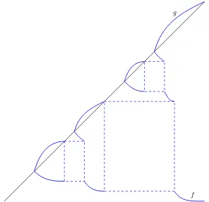
Figure 1: Stylized plot of the functionsf andgin the general (non-atomic) case. Note that on the set g(x) =xwe havef(x) =x.
Figure 1 gives a stylized representation off andg in the case whereν has no atoms. (Atoms ofν lead to horizontal sections off andg, see Section 4.1.) In the figure the set{g(x)> x}is a finite union of intervals whereas in general it may be a countable union of intervals. Similarly, in the figuref has finitely many downward jumps, whereas in general it may have countably many jumps. Nonetheless Figure 1 captures the essential behaviour off andg.
Remark 4. The left-curtain martingale coupling can be identified with Figure 1 in the following way: choose an x-coordinate according toµ; then ifg(x) =x setY =x=X so the pair (X, Y) lies on the diagonal; otherwise if g(x)> x thenf(x)< x and we set they-coordinate to be g(x) with probability
x−f(x)
g(x)−f(x) andf(x)with probability
g(x)−x
g(x)−f(x). Then the coordinates (x, y)represent the realised values of(X, Y).
For a horizontal levely there are two cases. Either, g(y)> y and then the value of y arises from a choice according toµof x=g−1(y)for which g(x) is chosen rather thanf(x); or g(y) =y and the valuey arises either from a choice according toµof x=y, or from a choice according toµ off−1(y) combined with a choice of y-coordinate off(f−1(y)) =y.
Suppose ν is also continuous and fix x. Then, by the first paragraph of Remark 4, under the left-curtain martingale coupling mass in the interval (f(x), x) at time-1 is mapped to the interval (f(x), g(x)) at time 2. Thus{f(x), g(x)} withf(x)≤x≤g(x) are solutions to
Z x
f
µ(dz) =
Z g
f
ν(dz), (10)
Z x
f
zµ(dz) =
Z g
f
Essentially, (10) is preservation of mass condition and (11) is preservation of mean and the martingale property. Ifν has atoms then (10) and (11) become
Z x
Returning to the case of continuousµ and ν, for fixed x there can be multiple solutions to (10) and (11). If, however, we considerf and g as functions ofxand impose the additional monotonicity properties of Lemma 3 (forx < x′,g(x)≤g(x′) and f(x′)∈/ (f(x), g(x))), then typically, for almost
allxthere is a unique solution to (10) and (11). However, there are exceptionalxat which f jumps and at which there are multiple solutions, see Section 3.2.
Remark 5. Note that ifg(x) =Tu(x) =x=f(x)> Td(x)then we typically do not haveR
Td(x)zν(dz). However, we trivially have
Rx
Remark 6. There are many pairs (µ, ν) which lead to the same pair of functions(f, g). Conversely, letI1⊆ I2⊆Rbe intervals and define any integrable measure with support inI1 and defineπviaπ(dx, dy) =µ(dx)χf(x),x,g(x)(dy)andν via
ν(dy) =
Z
x
µ(dx)χf(x),x,g(x)(dy). (14)
Then (subject to integrability conditions1) we have π∈Πˆ
M(µ, ν).
Mon, then provided the same integrability conditions are satisfied we have that if
ν is given by (14) thenπ given byπ(dx, dy) =µ(dx)χf(x),x,g(x)(dy)is the left-curtain mapping. The relevance of this remark is as follows. Given a pair µ≤cx ν it may be difficult to determine the properties of (f, g) which define the left-curtain coupling, beyond the fact that (f, g) ∈ ΞMon. (For example, it may be difficult to ascertain the number of downward jumps off without calculating
f and g everywhere.) However, if we want to construct examples for which (f, g) have additional properties (such as no downward jump) then we can start with an appropriate pair(f, g), take arbitrary (continuous) initial lawµwith support on the interval where f is defined, and then defineν via (14). This observation underpins our analysis in the next two sections.
3.1
American puts under the dispersion assumption
3.1.1 The left-curtain coupling
The goal in this section is to present the theory in a simple special case, and to illustrate the main features and solution techniques of our approach unencumbered by technical issues or the consideration
1We require that Rµ(dx)(g(x)−x)(x−f(x))
of exceptional cases. The following assumption is a small modification of one introduced by Hobson and Klimmek [16], see also Henry-Labord`ere and Touzi [12]. See Figure 2.
ρ
η
f e−
x g e+
Figure 2: Sketch of the densitiesρand η and the locations off, g for givenx > e−. Time-1 mass in
the interval (f, x) stays in the same place if possible. Mass which cannot stay constant is mapped to (f, e−) or (x, g) in a way which respects the martingale property.
Assumption 1(Dispersion Assumption). µandν are absolutely continuous with continuous densities
ρand η respectively. ν has support on (ℓν, rν)⊆(−∞,∞) and η >0 on (ℓν, rν). µ has support on
(ℓµ, rµ)⊆(ℓν, rν)andρ >0 on(ℓµ, rµ). In addition:
(µ−ν)+ is concentrated on an intervalE= (e
−, e+)andρ > η onE;
(ν−µ)+ is concentrated on(ℓ
ν, rν)\E andη > ρon(ℓν, e−)∪(e+, rν).
Ifµ≤cxν are centred normal distributions with different variances then Assumption 1 is satisfied.
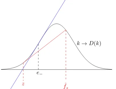
Under the Dispersion Assumption{k:Dµ,ν(k)>0}is an interval and D =Dµ,ν is convex to the
left ofe−, concave on (e−, e+) and again convex abovee+. See Figure 3.
k→D(k)
e−
ˆ fz
z
Figure 3: The function D. Under the dispersion assumption D(k) ≤ D(e−) + (k−e−)D′(e−) for
k≥e−.
Lemma 5. Suppose Assumption 1 holds. For all x∈(e−, rµ), there exist f, g with f < e− < x < g
such that(10)and (11)hold. Moreover, if we considerf andgas functions ofxon(e−, rµ)thenf and
limx↑rµf(x) = ℓν and limx↑rµg(x) = rν. Finally if we extend the domain of f and g to (ℓµ, rµ) by
settingf(x) =x=g(x)on (ℓµ, e−]then(f, g)∈Ξ(ℓMonµ,rµ),(ℓν,rν).
The proof of Lemma 5 is provided in the Appendix.
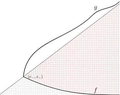
(e−, e−)
f g
Figure 4: Sketch of functionsf andgunder the Dispersion Assumption, with the regionsK2< f(K1)
andK2> f(K1) shaded. This is a simple special case of Figure 1.
Remark 7. As discussed at the end of Remark 6, for the purposes of the analysis of this section it is not the fact that the measures µ and ν satisfy the Dispersion Assumption which is important, but rather thatπlc is so simple, and{k:g(k)> k}is a single interval on which f is a monotone decreasing function.
Starting with monotonicfandg, lettingµbe continuous and definingνbyν(dy) =R
xµ(dx)χf(x),x,g(x)(dy) andπlc by
πlc(dx, dy) =µ(dx)δx(dy)I{x≤e−}+µ(dx)χf(x),x,g(x)(dy)I{x>e−}, (15) the pair (µ, ν) may or may not satisfy Assumption 1 but nonetheless, a candidate optimal model, stopping time and hedge can be constructed in exactly as described in this section, and can be proved to be optimal by the methods of this section.
Since our analysis depends on the pair (µ, ν) only through the functions(f, g) we may take as our starting point any(f, g)∈ΞMon.
Remark 8. Under the Dispersion Assumption (f, g)solve a pair of coupled differential equations on
[e−, rµ)obtained from differentiating (10) and (11):
df dx =−
g−x g−f
ρ(x) η(f)−ρ(f), dg
dx =
x−f g−f
ρ(x) η(g),
with the initial conditionf(e−) =e−=g(e−).
The principle being the left-curtain martingale couple in Beiglb¨ock-Juillet [4] is that we determine where to map mass atxat time-1 sequentially working from left to right. In our current setting there is an interval (ℓµ, e−] on which mass can remain unmoved between times-1 and 2. To the right ofe−
3.1.2 The American put
SupposeK1> e1. Define Λ : [g−1(K1), K1]7→Rby
Λ(x) =(K2−f(x))−(K1−x) x−f(x) −
(K1−x)
g(x)−x =
(g(x)−K1)
g(x)−x −
(K1−K2)
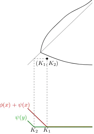
x−f(x) . (16) Pictorially Λ is the difference in slope of the two dashed lines in Figure 5.
K1
K2
f x g
slope (K2−f)−(K1−x)
x−f
slope (K1−x)
g−x
Figure 5: Sketch of put payoffs with pointsx,f and g marked. Λ(x) is the difference in slope of the two dashed lines.
Lemma 6. Suppose K1 > e− and f(K1) < K2. Then there is a unique x∗ = x∗(µ, ν;K1, K2) ∈
(g−1(K
1), K1)such that Λ(x∗) = 0.
Proof. It is clear, see Figure 6, that since f and g are continuous monotonic functions we have that Λ is continuous and strictly increasing. Moreover, Λ(g−1(K
1)) = −g−1(K1(K)−1(f−K◦g2−)1)(K1) < 0 and
Λ(K1) = KK21−−f(Kf(K11)) >0 by hypothesis. Hence there is a unique root to Λ = 0.
SupposeK1> e1andf(K1)< K2and thatx∗=x∗(µ, ν;K1, K2)∈(e1, K1) is such that Λ(x∗) = 0.
We define a martingale coupling as follows (the superscript∗ denotes the fact that the quantities we define are candidates for optimality):
Consider Ω∗ =R×R={ω = (ω1, ω2)} equipped with the Borel-sigma algebra F∗ =B(Ω∗). Let
(X, Y) be the co-ordinate process so thatX(ω) =ω1 andY(ω) =ω2. LetF0∗ be trivial and suppose F∗
1 =σ(X) and F2∗ =σ(X, Y). Finally, for ˆπ∈ΠM(µ, ν) letPˆπ be the martingale couplingPπˆ(X ∈
dx, Y ∈dy) = ˆπ(dx, dy) and setS∗ = (Ω∗,F∗,F∗:= (F∗
0,F1∗,F2∗),Pπˆ). Then (S∗, Mπˆ = (¯µ, X, Y)) is
a (µ, ν)-consistent model.
For anya < band a probability measureζ, letζa,b be the subprobability measure onR given by
ζa,b(A) =ζ(A∩(a, b)). Let ˜ζa,b=ζ−ζa,b.
It is easy to find a martingale coupling ofµandν such that (f(x∗), x∗) is mapped to (f(x∗), g(x∗)).
First notice that from the properties off andg(recall (10) and (11))µf(x∗),x∗andνf(x∗),g(x∗)have the
same mass and barycentre. Second notice they are in convex order. (One way to see this is to consider Dµf(x∗),x∗,νf(x∗),g(x∗)which is zero outside (f(x
∗), g(x∗)), convex on (f(x∗), e
−), concave on (e−, x∗) and
then convex again on (x∗, g(x∗)). HenceDµf(x∗),x∗,νf(x∗),g(x∗) ≥0 onR.) Hence there is a martingale
coupling of µf(x∗),x∗ and νf(x∗),g(x∗). Moreover, ˜µf(x∗),x∗ and ˜νf(x∗),g(x∗) also must have common
mass and mean under the Dispersion Assumption, and are in convex order (D˜µf(x∗),x∗,˜νf(x∗),g(x∗) is
convex on (−∞, f(x∗)), concave on (f(x∗), g(x∗)∨e
+) and convex on (g(x∗)∨e+,∞) and hence
Dµ˜f(x∗),x∗,˜νf(x∗),g(x∗) ≥0.) Then we can define a martingale coupling of µ and ν by combining the
that the left-curtain martingale coupling of Beiglb¨ock and Juillet [4] maps (f(x∗), x∗) to (f(x∗), g(x∗))
and the complement of (f(x∗), x∗) to the complement of (f(x∗), g(x∗)).)
Let ˆπx∗ ∈ ΠˆM(µ, ν) be any martingale coupling such that ˆπx∗ maps (f(x∗), x∗) to (f(x∗), g(x∗))
and (f(x∗), x∗)Cto (f(x∗), g(x∗))C. LetM∗= (M∗
0 = ¯µ, M1∗=X, M2∗=Y) be the stochastic process
such thatP(X ∈ dx, Y ∈dy) = ˆπx∗(dx, dy). Then M∗ ∈ M(S∗, µ, ν). Letτ∗ be the stopping time
such thatτ∗= 1 on (−∞, x∗) andτ∗ = 2 otherwise. Our claim in Theorem 1 below is that (S∗, M∗)
and the stopping timeτ∗are such that the model-based price of the American put under this stopping
time is the highest possible, over all consistent models.
Continue to suppose K1 > e− and f(K1) < K2. Now we define a superhedge. Let ψ∗ be the
function
ψ∗(z) =
(K2−z) z≤f(x∗) (g(x∗)−z)(K
2−f(x∗))
g(x∗)−f(x∗) f(x
∗)< z≤g(x∗)
0 z > g(x∗)
(17)
Note that by construction and by (16), K2−f(x∗)
g(x∗)−f(x∗)= K1−x∗
g(x∗)−x∗ and thenψ(x∗) =K1−x∗. Moreover,
ψis convex and by Lemma 2,ψ∗ can be used to construct a superhedge (ψ∗, φ∗, θ∗
1,2).
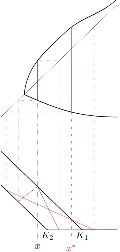
x∗
x
K1
K2
Figure 6: A combination of Figures 4 and 5, showing how jointly they define the best model and best hedge. By adjustingxwe can findx∗ such that Λ(x∗) = 0. Together the quantities (f(x∗), x∗, g(x∗))
define the optimal model, stopping time and hedge.
Theorem 1. Suppose Assumption 1 holds.
1. Suppose K1> e− andf(K1)< K2. The model(S∗, M∗)described in the previous paragraphs is a consistent model for which the price of the American option is highest. The stopping timeτ∗
is the optimal exercise time. The function ψ∗ defined in (17) defines the cheapest superhedge. Moreover, the highest model-based price is equal to the cost of the cheapest superhedge.
2. Suppose K1 ≤ e− or K1 > e− and f(K1) ≥ K2. Then there is a consistent model for which
rule τ = 1 if X < K1 and τ = 2 otherwise attains the highest consistent model price. The cheapest superhedge is generated from ψ(x) = (K2−x)+ and the highest model-based price is equal to the cost of the cheapest hedge.
Proof. Suppose K1> e− and f(K1) < K2. Then by Lemma 6 there is a unique x∈(g−1(K1), K1)
such that Λ(x) = 0. For thisxwe can findf =f(x) andg=g(x) withf < K2 andK1< g such that K2−f
g−f = K1−x
g−x . Since ν is continuous we have thatf, x, g solve (10) and (11). The elements f, x, g
can be used to define a model using the construction after Lemma 6 above. For this model we can calculate the expected payoff of the American put. At the same time we can use (f(x), x, g(x)) to define a superhedge. The remaining task is to show that the cost of the superhedge equals that of the model-based expected payoff. Then by the discussion in Section 2.4 we have found an optimal model and cheapest superhedge.
Recall thatPχ(k) =R−∞k (k−x)χ(dx),χ∈ {µ, ν}, and thatD(k) =Dµ,ν(k) =Pν(k)−Pµ(k). (10)
and (11) can be rewritten as
P′
µ(x)−Pµ′(f) = Pν′(g)−Pν′(f) (18)
(xPµ′(x)−Pµ(x))−(f Pµ′(f)−Pµ(f)) = (gPν′(g)−Pν(g))−(f Pν′(f)−Pν(f)) (19)
In the model the candidate strategy is to exercise the American put at time 1 if and only if the underlying is belowx. Note that under the candidate model mass belowf at time 1 is mapped to the same point at time 2, and mass in (f, x) is mapped to (f, g). Mass abovexis either mapped to below f (there is massν−µto be embedded there) or to aboveg. The expected payoff of the American put (for this model and stopping rule) is
Z x
−∞
(K1−w)+µ(dw) +
Z f
−∞
(K2−w)+(ν−µ)(dw) =Pµ(x) + (K1−x)Pµ′(x) +D(f) + (K2−f)D′(f).
Now we consider the hedging cost. Set Θ =K2−f
g−f ∈(0,1). Note that, sincexis such that Λ(x) = 0
we have Θ =K1−x
g−x . Letψ(y) be given by
ψ(y) = Θ(g−y)++ (1−Θ)(f −y)+
and note thatψ(y) = (K2−y) fory ≤f, andψ(y)≥(K2−y)+ in general. Using Lemma 2 we can
useψ to generate a superhedging strategy. The cost of this strategy is
ΘPν(g)+ (1−Θ)Pν(f)+ (1−Θ) [Pµ(x)−Pµ(f)] =Pµ(x)+D(f)+ Θ [Pν(g)−Pν(f)−Pµ(x) +Pµ(f)].
Now we consider the difference between the hedging cost (HC) and the model-based expected payoff (M BEP):
HC−M BEP = Θ [Pν(g)−Pν(f)−Pµ(x) +Pµ(f)]−(K1−x)Pµ′(x)−(K2−f)D′(f)
= Θ
gPν′(g)−xPµ′(x)−f D′(f)
−(K1−x)Pµ′(x)−(K2−f)D′(f)
= Θ
(g−x)Pµ′(x) + (g−f)D′(f)
−(K1−x)Pµ′(x)−(K2−f)D′(f)
= P′
µ(x) [Θ(g−x)−(K1−x)] +D′(f) [Θ(g−f)−(K2−f)]
= 0
where we use (19), (18) and the definition of Θ respectively. Optimality of the model, stopping rule and hedge now follows.
Now supposeK1≤e−. Consider an exercise rule in which the American put is exercised at time-1
(K1, K2)
K1
K2
ψ(y) φ(x) +ψ(x)
Figure 7: Sketch of put payoffs with ψ(y) = (K2−y)+ andφ(x) = (K1−x)+−(K2−x)+.
stays constant between times 1 and 2. (This is possible sinceµ≤ν on (−∞, e−) andK1≤e−.) The
expected payoff of the American put is
Z K1
−∞
(K1−x)µ(dx) +
Z K2
−∞
(K2−y)(ν−µ)(dy) =Pµ(K1) +Pν(K2)−Pµ(K2).
Alternatively, suppose K1 > e− but f(K1)≥ K2. Then under the left curtain martingale coupling
mass belowK2 at time 1 stays constant between times 1 and 2 (note that K2 ≤f(K1)≤e−), and
mass betweenK2 andK1 at time 1 is mapped to (K2,∞). Then, mass which is belowK2 at time 2
was either belowK2at time 1, or aboveK1at time 1. The expected payoff under this model (using a
strategy of exercising at time 1 if the American put is in the money) is again
Z K1
−∞
(K1−x)µ(dx) +
Z K2
−∞
(K2−y)(ν−µ)(dy) =Pµ(K1) +Pν(K2)−Pµ(K2).
Conversely, letψ(y) = (K2−y)+. Definingφas in Lemma 2 we findφ(x) = (K1−x)+−(K2−x)+=
(K1−(x∨K2))+ and the superhedging cost is
HC =Pν(K2) +Pµ(K1)−Pµ(K2).
Hence the model-based expected payoff equals the hedging cost.
3.2
Two intervals of
g > x
and one downward jump in
f
We now relax the Dispersion Assumption to the case wheref is not monotone. The simplest situation when this may arise is when there are two intervals on which g(x) > x. We do not contend that there are many natural examples which fall into this situation, but rather that this intermediate case illustrates phenomena which are to be found in the general case but which were not to be found under the Dispersion Assumption.
on(ℓµ, rµ)⊆(ℓν, rν)andρ >0 on(ℓµ, rµ). In addition:
3. gis continuous and strictly increasing;
4. f(x) =xon (ℓµ, e−1]∪[x′, e2−];
f′ zν(dz). In particular, given (20) and (21), the pair of equations
Z x′′
has two solutions for f, namelyf =x′ and f = f′. Hence, in defining the left-curtain martingale
coupling there are two choices for f at x′′: we may take f(x′′) = x′ or f(x′′) = f′. Rather than
assuming one of these choices (for example by requiring left-continuity off) it is convenient to allow f to be multi-valued. Then, forxsuch thatg(x)> xletℵ(x) ={f : (f, x, g(x)) solves (10) and (11)}. Then, in the setting of Assumption 2, for x > e−, |ℵ(x)| = 1 except at x′′ and there ℵ(x′′) =
{f(x′′+), f(x′′−)}={f′, x′}.
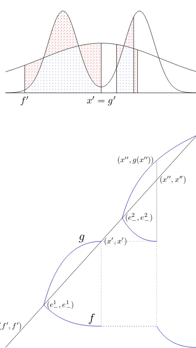
Remark 9. As discussed in Remark 6 when constructing examples which fit with the analysis of this section, we may begin with f, g as presented in the bottom half of Figure 8. Given µ with support
f′ x′ =g′
(f′, f′)
(e1 −, e1−)
(x′, x′)
(e2 −, e2−)
(x′′, x′′)
(x′′, g(x′′))
g
f
Figure 8: Picture off andg under Assumption 2.
Remark 10. Recall Remark 8 and the principle that quantities in the left-curtain mapping are deter-mined working from left to right. Given thatµ andν have continuous densities and given that η > ρ
on(ℓµ, e1−)we can set f =g=xon this interval. To the right ofe1− we haveρ > ηand we can define
f and g using the differential equations in Remark 8. There are two cases, either g(x) > x for all
x∈(e1
−, rµ)(in which case we can define(f, g)on(e1−, rµ) with the properties described in Lemma 5) or there is some point at whichg first hits the diagonal liney=xagain. This point is exactlyx′.
If x′ exists it must satisfyx′ ∈(e1
+, e2−). Then we setg(x) =xon (x′, e2−)and let f =g solve the
same coupled differential equations as in Remark 8 but with a new starting pointg(e2
−) =e2−=f(e2−).
The ODEs determine f andg until f first reaches x′. This happens at x′′, and at x′′ f jumps down
tof′ (andg is continuous). To the right of x′′, f andg solve the differential equations again subject
to initial conditionsf(x′′) =f′,g(x′′) =g(x′′−).
Recall the definition Λ(x) = g(x)−K1
g(x)−x −
(K1−K2)
(x−f(x)). If f is valued, then Λ will also be
Introduce Υ = ΥK1,K2(f, x, g) which is defined forf ≤K2, x≤K1≤g by
g(x′′)−x′′. This motivates the introduction of the linear increasing functionsLu,
Ld: [x′′, g(x′′)]→Rdefined by
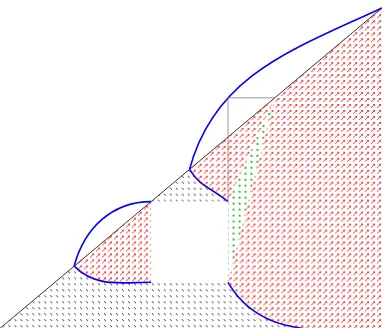
Pictorially,Ld andLu are the lower and upper boundaries respectively, of the dotted triangular area Gin Figure 9.
From Figure 9 we identify four regions (and various subregions) on which four different martingale couplings and hedging strategies will be needed in order to find the highest model-based expected payoff of American put. (Compare this with two regimes under the Dispersion Assumption in Figure 4.)
i=1RiandB=∪3i=1Ri. In general, on the boundaries between the regions the boundaries
could be allocated to either region. However, we allocate points on the boundary to the region where the hedge is simplest.
Λ(x) = Υ(f(x), x, g(x)) is also continuous. Then the same argument as in the proof of Lemma 6 shows that there exists a uniquex∗=x∗(µ, ν;K
1, K2)∈(g−1(K1), K1) such that Λ(x∗) = 0.
Now suppose (K1, K2)∈ R3∪R4and consider Λ as before. Recall that Λ is increasing, Λ(g−1(K1))<
0 and Λ(K1)>0. On the other hand,g−1(K1)< x′′and hence Λ has an upward jump atx′′ (since f
has a downward jump atx′′). There are two cases depending on whether (K
1. SupposeK2 > Lu(K1). Then Λ(x′′−) >0. Since Λ(g−1(K1)) <0, by the continuity of Λ on
(g−1(K
1), x′′), there exists a uniquex∗ =x∗(µ, ν;K1, K2)∈(g−1(K1), x′′) such that Λ(x∗) = 0.
IfK2=Lu(K1) then Υ(x′, x′′g(x′′)) = 0 and we takex∗=x′′,g∗=g(x′′) andf∗=f(x′′−) =x′.
2. Suppose K2 < Ld(K1). Then Λ(x′′+) < 0. Further, since Λ(K1) > 0 there exists a unique
x∗ =x∗(µ, ν;K
1, K2)∈(x′′, K1) such that Λ(x∗) = 0. IfK2=Ld(K1) then Υ(f′, x′′, g(x′′)) = 0
and we takex∗=x′′,g∗=g(x′′) andf∗=f(x′′+) =f′.
Figure 9: Picture off and g in bi-modal case, now with 4 regions shaded (cross-hatched, diagonally, dotted and blank).
By Lemma 7, for (K1, K2)∈ Rthere exists{f∗∈ ℵ(x∗), x∗, g∗=g(x∗)}such that Υ(f∗, x∗, g∗) = 0.
Suppose (K1, K2)∈ R1∪ R4∪ R5. As before, letM∗= (M0∗= ¯µ, M1∗=X, M2∗=Y) be the stochastic
process such thatP(X∈dx, Y ∈dy) = ˆπx∗(dx, dy), where ˆπx∗ ∈Π(µ, ν) is a martingale coupling thatˆ
combines the couplingsµf∗,x∗ 7→νf∗,g∗ and ˜µf∗,x∗ 7→ν˜f∗,g∗.
Recall the proof of Theorem 1. There, to show thatM BEP =HC, we used the fact that under modelM∗, or more specifically, under any martingale coupling which mapped (f∗, x∗) to (f∗, g∗), the
mass that is unexercised at time 1 and is in the money at time 2 is given by (ν−µ)|(−∞,f∗) where
f∗< e
−. Whenf(x′)< e1−(as is the case when (K1, K2)∈ R1∪ R4∪ R5) then the same proof applies,
M BEP =HC and we have optimality. However, if (K1, K2)∈ R2∪ R3, then it is not the case that
f∗< e1
− and thus, in order to specify the optimal model, we need to impose additional structure on
the coupling ˜µf∗,x∗ 7→ν˜f∗,g∗.
Suppose (K1, K2) ∈ R2∪ R3. Then x′ < f∗, so that (f′, x′)∩(f∗, g∗) = ∅. From the defining
properties off′andx′we see that there exists a martingale coupling, which we term ˆπ
x′,x∗ ∈ΠˆM(µ, ν),
that combines the couplings of µf′,x′ 7→ νf′,x′ and µf∗,x∗ 7→ νf∗,g∗, so that ˆπx′,x∗ maps (f′, x′) to
(f′, x′), (f∗, x∗) to (f∗, g∗) and ((f′, x′)∪(f∗, x∗))C to ((f′, x′)∪(f∗, g∗))C. Let ˆM∗ = ( ˆM∗
0 =
¯ µ,Mˆ∗
1 =X,Mˆ2∗=Y) be the stochastic process such that P(X ∈dx, Y ∈dy) = ˆπx′,x∗(dx, dy).
If (K1, K2)∈ R1∪ R4∪ R5 we haveM∗ ∈ M(S∗, µ, ν) and if (K1, K2)∈ R3∩ R4 we have that
ˆ
M∗ ∈ M(S∗, µ, ν). For both models we consider a candidate stopping time τ∗ = 1 if X < x∗ and
τ∗ = 2 otherwise, and a candidate superhedge (ψ∗, φ∗, θ∗
1,2) generated by the function ψ∗ defined in
(17).
the cheapest superhedge. Moreover, the highest model-based price is equal to the cost of the cheapest
Then under the candidate stopping ruleτ∗the model-based expected payoff is equal to the cost of the
hedging strategy generated byψ∗:
M BEP =
ifX < K1 andτ = 2otherwise attains the highest consistent model price. The cheapest superhedge is generated fromψ(x) = (K2−x)+ and the highest model-based price is equal to the cost of the cheapest hedge.
Proof. Letψ(y) = (K2−y)+. Definingφas in Lemma 2 we find φ(x) = (K1−x)+−(K2−x)+ and
the superhedging cost (which is the same for all the cases) is
Suppose (K1, K2)∈ B1. Then using the properties off andg and the left-curtain coupling we see
that the proof that the model-based expected payoff is equal to the hedging cost is the same as in the second case of Theorem 1. In particular,
M BEP =
mapped to the same interval at time 2. Therefore mass which is belowK2 at time 2 was either below
K2 at time 1, or abovex′ at time 1. Therefore, we again have
Finally, suppose (K1, K2)∈ B3. We again utilise the fact that under the left-curtain coupling, mass
(K1, K2)
f′ x′
ψ
x′Figure 10: Picture off andg along with superhedge for the blank regionW.
Theorem 4. Suppose Assumption 2 holds and (K1, K2)∈ W.
Then there is a consistent model for which(f′ < X < x′) = (f′ < Y < x′) and any model with this
property with the stopping rule τ = 1 if X < K1 and τ = 2otherwise attains the highest consistent model price. The cheapest superhedge is generated fromψx′
defined in (24) and the highest model-based price is equal to the cost of the cheapest hedge.
Proof. First note that
ψx′(z) = Θ(x′−z)++ (1−Θ)(f′−z)+, where Θ = K2−f′
x′−f′. Sincex
′ < K
1 we have
φx′(w) +ψx′(z) = (K1−w)+−ψx ′
(w) +ψx′(z)
= (K1−w)++ Θ[(x′−z)+−(x′−w)+] + (1−Θ)[(f′−z)+−(f′−w)+]
and the cost of this strategy (under any consistent model) isHC=Pµ(K1) + ΘD(x′) + (1−Θ)D(f′).
Now consider the model-based expected payoff. From (20) it follows thatµf′,x′ andνf′,x′ have the
same mean and mass, and are in convex order. Moreover, the same holds for ˜µf′,x′ and ˜νf′,x′. Hence
there exists a martingale coupling, which we term ˆπx′
∈ΠˆM(µ, ν), which maps the mass in (f′, x′) at
Note that, sincef′ andx′ satisfy (20), and henceRx′
respectively. Then we define a martingale coupling ˆπx′,x′′ ∈ Π(µ, ν) by combining the couplings ofˆ
µf′,x′ 7→ νf′,x′, µx′,x′′ 7→ νx′,g(x′′) and (˜µf′,x′−µx′,x′′) 7→(˜νf′,x′−νx′,g(x′′)). In other words, ˆπx′,x′′
used in the proof of Theorem 4.
Given x′, and thus also x′′, we define the superhedge as follows. First define linear functions
∆1: [f′, x′]→Rand ∆2: [x′, g(x′′)]→Rby
direct calculation shows that−1<∆′
(K1, K2)
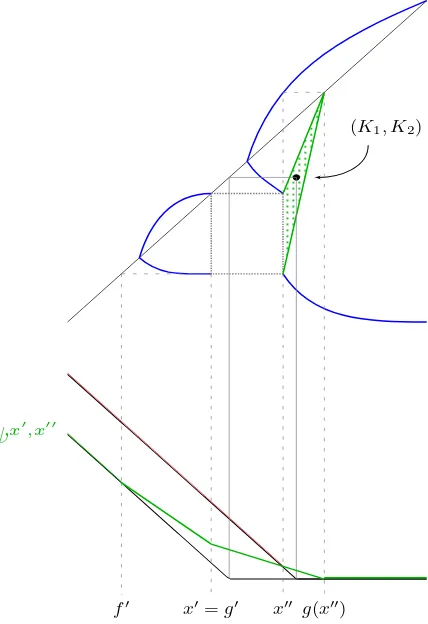
g(x′′) x′′ f′
ψ
x′,x′′x′=g′
Figure 11: Picture off and g along with superhedge for the dotted region G. The hedge function Ψx′,x′′ has a kink atx′.
Theorem 5. Suppose Assumption 2 holds and (K1, K2) ∈ G. The model Mx ′,x′′
and the stopping timeτ= 1ifX < x′′ andτ = 2otherwise attains the highest consistent model price. Moreover,ψx′,x′′ defined in (25)generates the cheapest superhedge and the highest model-based price is equal to the cost of the cheapest superhedge.
Proof. Under the candidate modelMx′,x′′
mass in (f′, x′) at time 1 is mapped to the same interval at
time 2, while the mass in (x′, x′′) is mapped to (x′, g(x′′)). Then under the candidate stopping time
(exercise at time 1 ifX < x′′and at time 2 otherwise) the law ofY (underMx′,x′′
) on the event that the option was not exercised at time 1 is given by (ν−µ)|(−∞,f′)+ν|(g(x′′),∞). Therefore
M BEP =
Z x′′
−∞
(K1−w)+µ(dw) +
Z f′
−∞
(K2−w)+(ν−µ)(dw)
=Pµ(x′′) + (K1−x′′)Pµ′(x′′) +D(f′) + (K2−f′)D′(f′).
Now consider the hedging cost generated by ψx′,x′′
. Let Θ1 = K2−f ′−∆
2(x′)
x′−f′ = −∆
′
1 and Θ2 = K1−x′′
g(x′′)−x′′ =−∆′2. Note that we can rewrite (25) asψx ′,x′′
(z) = Θ2(g(x′′)−z)++ (Θ1−Θ2)(x′−z)++
(1−Θ1)(f′−z)+ . Then
φ(z) = (1−Θ1)[(x′−z)+−(f′−z)+] + (1−Θ2)[(x′′−z)+−(x′−z)+],
and thus the hedging cost is
HC = Θ2Pν(g(x′′)) + (1−Θ1)D(f′) + (1−Θ2)Pµ(x′′) + (Θ1−Θ2)D(x′)
Now using (20) and the fact that g(x′) = x′ we have that D′(f′) =D′(x′) andf′D′(f′)−D(f′) =
x′D′(x′)−D(x′). Hence
Θ1[D(x′)−D(f′)] = (K2−f′)D′(f′)−∆2(x′)D′(f′); (26)
moreover (21) gives that
Θ2[Pν(g(x′′))−Pν(x′)−Pµ(x′′) +Pµ(x′)]
= Θ2[g(x′′)Pν′(g(x′′))−x′′Pµ′(x′′)−x′D′(x′)]
= Θ2[(g(x′′)−x′′)Pµ′(x′′) + (g(x′′)−x′)D′(x′)]
= (K1−x′′)Pµ′(x′′) + ∆2(x′)D′(f′). (27)
Then, combining (26) and (27) we conclude thatHC=M BEP.
3.3
The general case for continuous
µ
In the previous sections we showed how the left-curtain coupling can be used to find an optimal model, exercise strategy and a superhedge, under the assumption that bothµandν are continuous together with further regularity and simplifying assumptions which we labelled the Dispersion Assumption and the Single Jump Assumption. Under the latter assumption, the existence of points that solve (20) led us to identify two further types of hedging strategy that were not present under dispersion assumption, making four in total.
If we relax the assumptions further and require only that both µ and ν are continuous, then we expect that there exist multiple pairs (f′
i, x′i), i = 1,2,3, ..., that solve (20). Note that from the
monotonicity of g we can write {x : g(x) > x} as countable union of intervals, and on each such interval f is decreasing. f jumps over the intervals (f′
i, x′i) identified above (at least those with x′
to the left of the current value of x). In particular, f has only countably many downward jumps. Figure 1 is a stylized representation of the general left-curtain martingale coupling, not least because in the figuref has only finitely many jumps. Using Figure 1 we can divide (K1, K2< K1) into four
regions, see Figure 12. They key point is that these four regions are characterised exactly as in the case described in Section 3.2. For given (K1, K2) we can determine which of the types of hedging strategy
is a candidate optimal superhedge, and determine a candidate optimal stopping rule. (We can always use the model associated with the left-curtain martingale couplingπlc.) The fact that these candidates
Figure 12: General picture of f, g with shading of regions. There remain 4 types of shading corre-sponding to 4 forms of optimal hedge.
More specifically, we can divide (k2 < k1) into (k2 ≤f(k1))∪(f(k1)< k2 < k1). We can divide
the former into two regions W = {(k2, k1) : (k2 < k1);∃x ≤ k1such thatf(x)< k2< g(x)} and B= (k2< k1)\ W. The latter we again divide into two regionsGandR= (f(k1)< k2< k1)\ G. Here
we can write G = ∪x:f(x−)>f(x+)∆(x) where ∆(x) is a triangle with vertices (x, f(x+)), (x, f(x−)
and (g(x), g(x)). Then on each of the regions W, B, G and R we have a superhedge exactly as described in Section 3.2. Moreover, again by the arguments of Section 3.2, we can show that the hedging cost associated with the super-hedging strategy is precisely the model-based expected payoff of the American put under the martingale couplingπlc (and candidate stopping rule) thus proving the
optimality of the hedge and of the model/exercise rule.
4
Discussion and extensions
4.1
Atoms in the target law
Whenν has atoms, the preservation of mass and mean conditions become (12) and (13), respectively. In particular, atoms of ν correspond to the flat sections in f or g. See Figure 13. In this case we still can find all the optimal quantities as before. In particular, Λ(x) := g(x)−K1
g(x)−x −
(K1−K2)
x−f(x) is strictly
increasing inx, even iff and/org is constant. Hence we can find solutions to Λ = 0 (more generally solutionsx, f ∈ ℵ(x) to Υ(f, x, g=g(x)) = 0) exactly as before. The superhedge is unchanged. A little care is needed in constructing the optimal model, but mass in (f(x∗), x∗) is mapped to (f(x∗), g(x∗))
together with (potentially) atoms atf(x∗) org(x∗). Specifically, givenf∗, x∗, g∗ we can findλ∗
f and
λ∗g such that (12) and (13) hold. Then, in any optimal model mass in (f∗, x∗) is mapped toνx∗ which
x1 x2
0< ν({x2})
0< ν({x1})
g(ˆx−) g(ˆx+)
f(¯x−) f(¯x+)
Figure 13: Atoms ofν correspond to flat sections in f andg. Regions of no mass ofν correspond to jumps off andg.
4.2
Intervals where
ν
has no mass, or
ν
=
µ
.
The definition of the left-curtain martingale coupling (recall Lemma 5) only requires thatg =Tu is
increasing, and not that it is continuous. In generalg may have jumps; such jumps occur when there is an interval on whichν places no mass.
Ifghas a jump then we need to adapt the superhedge. Supposeghas a jump at ˆx(which has to be upwards sincegis increasing), and supposef is continuous at ˆx. Suppose further thatK1is such that
ˆ
x∈(g−1(K
1), K1). Then as before, we would like to find x∗ ∈ (g−1(K1), K1) such that Λ(x∗) = 0.
Recall that Λ is increasing and suppose Λ(g−1(K
1)) < 0 < Λ(K1). If Λ(ˆx−) < 0 and Λ(ˆx+) > 0,
then there will be no solution to Λ = 0. On the other hand, by keeping x = ˆx,fˆ= f(ˆx) fixed in (16), and varyingg only, we see that there exists ˆg ∈(g(ˆx−), g(ˆx+)), such that (ˆg−K1)/(ˆg−x) =ˆ
(K1−K2)/(ˆx−fˆ) so that Υ(f(ˆx),ˆx,ˆg) = 0. Then, the candidate (and indeed optimal) superhedging
strategy is generated byψ∗, given in (17), with (f∗, x∗, g∗) = ( ˆf ,ˆx,ˆg), see Figure 14. Moreover, sinceν
does not charge (g(ˆx−), g(ˆx+)), the triple ( ˆf ,x,ˆ ˆg) solves the mass and mean equations (10) and (11). The strong duality between the model-based expected payoff and the hedging cost follows as before.
K1
K2
ˆ
f xˆ g(ˆx−) gˆ g(ˆx+)
Alternatively, supposef has a downward jump at ¯x. This can happen ifν =µon (f(¯x+), f(¯x−)). For both jumps inf andg, we have a pictorial representation of the regions of pairs (K1, K2) which
lead to a hedging strategy which has to be adapted as above, see Figure 13. If g has a jump at ˆx, then Λ(ˆx−)<0 and Λ(ˆx+)>0 is equivalent to point (K1, K2) lying in the interior of a triangle with
4.3
The role of the left-curtain coupling
For any pair of strikes (K1, K2) the left-curtain model attains the highest expected payoff for the
American put. However, although it optimises simultaneously across all pairs of strikes it is not (in general) optimal for linear combinations of American puts. For example, if we consider a generalised American option with payoff a if exercised at time-1 and b if exercised at time-2, where a(x) =
PJ
1 for each j), then the model associated
with the left-curtain coupling is typically not optimal. The reason is that a model (S, M) is only optimal when it is combined with the best stopping rule, and the optimal stopping ruledoes depend on (K1, K2).
Conversely, although the model associated with the left-curtain coupling is optimal (simultaneously across all pairs K1, K2), we do not need the full power of this coupling when we work with fixed
(K1, K2). In the dispersion assumption case all we need is a coupling in which (f(x∗), x∗) is mapped
to (f(x∗), g(x∗)) wherex∗ is such that Λ(x∗) = 0. There are many martingale couplings which have
this property.
The intuition behind the optimality of the left-curtain coupling is as follows. With American puts there is a tension between the time-decay of the option payout encouraging early exercise, and the convexity of the payoff function promoting delay. If the aim is to maximise the payoff of the option then any paths which are in the money at time one, and will remain in the money, are best exercised at time-1. However, once a path has been exercised, any further volatility is wasted. In particular, when designing a candidate optimal model we should try to keep paths which are exercised at time-1 constant (or near constant) whenever possible. Thus the probability space should be split into two regions: one region where the put is in-the-money at time-1 and is exercised, and thereafter paths move little, and a second region where the put is out-of-the-money at time-1 (and sometimes just in-the-money, but left unexercised at time-1) and then there is a large jump between times 1 and 2.
References
[1] Az´ema J., Yor M.: Une solution simple au probleme de Skorokhod. InS´eminaire de probabilit´es XIII, pages 90–115. Springer, 1979.
[2] Bayraktar E., Huang Y-J., Zhou Z.: On hedging American options under model uncertainty.
[3] Beiglb¨ock M., Henry-Labord`ere P., Penkner F.: Model-independent bounds for option prices—mass transport approach. Finance and Stochastics, 17(3):477–501, 2013.
[4] Beiglb¨ock M., Juillet N.: On a problem of optimal transport under marginal martingale con-straints. The Annals of Probability, 44(1):42–106, 2016.
[5] Billingsley P.: Convergence of probability measures. John Wiley & Sons, 2013.
[6] Breeden D.T., Litzenberger R.H.: Prices of state-contingent claims implicit in option prices.
Journal of Business, pages 621–651, 1978.
[7] Brown H., Hobson D.G., Rogers L.C.G.: Robust hedging of barrier options. Mathematical Finance, 11(3):285–314, 2001.
[8] Carr P., Lee R.: Hedging variance options on continuous semi-martingales.Finance and Stochas-tics, 14(2):179–207, 2010.
[9] Cox A.M.G., Hoeggerl C.: Model-independent no-arbitrage conditions on American put options.
Mathematical Finance, 26(2):431–458, 2016.
[10] Cox A.M.G., Ob l´oj J.: Robust pricing and hedging of double no-touch options. Finance and Stochastics, 15(3):573–605, 2011.
[11] Cox A.M.G., Wang J.: Optimal robust bounds for variance options. arXiv preprint arXiv:1308.4363, 2013.
[12] Henry-Labord`ere P., Touzi N.: An explicit martingale version of the one-dimensional Brenier theorem. Finance and Stochastics, 20(3):635–668, 2016.
[13] Herrmann S., Stebegg F.: Robust pricing and hedging around the globe. arXiv preprint arXiv:1707.08545, 2017.
[14] Hobson D.G.: Robust hedging of the lookback option. Finance and Stochastics, 2(4):329–347, 1998.
[15] Hobson D.G.: The Skorokhod embedding problem and model-independent bounds for option prices. In Paris-Princeton Lectures on Mathematical Finance 2010, pages 267–318. Springer, 2011.
[16] Hobson D.G., Klimmek M.: Robust price bounds for the forward starting straddle. Finance and Stochastics, 19(1):189–214, 2015.
[17] Hobson D.G., Neuberger A.: Robust bounds for forward start options. Mathematical Finance, 22(1):31–56, 2012.
[18] Hobson D.G., Neuberger A.: On the value of being American. Finance and Stochastics, 21(1) 285–329, 2017.
[19] Hobson D.G., Neuberger A.: More on hedging American options under model uncertainty. arXiv preprint arXiv:1604.02274, 2016.
[20] Hobson D.G., Norgilas D.: The left curtain martingale coupling in the presence of atoms. In preparation.
[21] Neuberger A.: Bounds on the American option. Preprint SSRN:966333, 2007.
A
Proofs
Proof of Lemma 5. We provide a graphical construction of the left-curtain mapping under the Disper-sion Assumption.
Forx≤e− we setf(x) =x=g(x). Note that this choice off andg trivially satisfies the mass and
mean conditions (10) and (11), respectively.
Fixx > e−. First we want to show that there existsf < x < gsatisfying mass and mean conditions.
Secondly, as functions ofxwe want to show thatf is decreasing andg is increasing. Forz < e− introducePν,z(k) by
Pν,z(k) =
Z k
z
(k−x)ν(dx) +
Z z
−∞
(k−x)µ(dx)
= Pν(k)− {D(z) + (k−z)D′(z)} (28)
= Pµ(k) +{D(k)−D(z)−(k−z)D′(z)}. (29)
Since D(·) is non-negative and D′(z) > 0, from (28) we have thatP
ν,z(k) < Pν(k) for k > z. Set
LD,z(k) = D(k)−D(z)−(k−z)D′(z) and note that equation LD,z(k) = 0 has two (finite) roots,
k=z andk= ˆfz > e− (recall Figure 3), so thatD(k)≥D(z) + (k−z)D′(z) fork≤fˆz andD(k)<
D(z) + (k−z)D′(z) fork >fˆ
z. Therefore from (29) we have thatPν,z(z) =Pµ(z),Pν,z( ˆfz) =Pµ( ˆfz),
P′
ν,z(z) =Pµ′(z),Pν,z(k)> Pµ(k) fork <fˆzandPν,z(k)< Pµ(k) fork >fˆz. Also, for ˜z < z < e−
Pν,˜z(k)−Pν,z(k) =
Z z
˜ z
(k−x)[ν(dx)−µ(dx)]>0, k > z,
and in particular, for anyk0> z,
Pν,˜z(k)−Pν,z(k) =A(k−k0) +B, k > z, (30)
whereA >0 andB >0 are given by
A=
Z z
˜ z
[ν(dx)−µ(dx)], B=Pν,˜z(k0)−Pν,z(k0).
LetLx be the tangent to Pµ at x. The idea is to use the fact thatPν,z is monotonic in z on the
domain (e−,∞) and to adjust z until Lx is also tangent to Pν,z at some g > x. If z ≤ ℓν, then
Pν,z(k) =Pν(k)> Pµ(k)> Lx(k) fork > x, and soLxis not a tangent toPν,z. On the other hand, for
eachx > e−there exists a uniquezx< e−such that ˆfzx =xand thenPν,fˆzx(x) =Pµ(x) =Lx(x). Note
thatD′(z
x)> D′(k) for anyk≥x, and therefore Pν,z′ x(x)< P
′
µ(x) =L′x(x). HencePν,zx(k)< Lx(k)
for not too largek > x, and Lxis not tangent to Pν,fˆ