isprs archives XLII 3 W3 65 2017

(1)

REVISITING EXISTING CLASSIFICATION APPROACHES FOR BUILDING

MATERIALS BASED ON HYPERSPECTRAL DATA

R. Ilehag∗_{, M. Weinmann, A. Schenk, S. Keller, B. Jutzi, S. Hinz}

Institute of Photogrammetry and Remote Sensing, Karlsruhe Institute of Technology (KIT), Englerstr. 7, 76131 Karlsruhe, Germany -(rebecca.ilehag, martin.weinmann, andreas.schenk, sina.keller, boris.jutzi, stefan.hinz)@kit.edu

Commission III, WG III/4

KEY WORDS:Hyperspectral data, Building facades, Feature selection, Classification, Urban materials

ABSTRACT:

Classification of materials found in urban areas using remote sensing, in particular with hyperspectral data, has in recent times increased in importance. This study is conducting classification of materials found on building using hyperspectral data, by using an existing spectral library and collected data acquired with a spectrometer. Two commonly used classification algorithms, Support Vector Machine and Random Forest, were used to classify the materials. In addition, dimensionality reduction and band selection were performed to determine if selected parts of the full spectral domain, such as the Short Wave Infra-Red domain, are sufficient to classify the different materials. We achieved the best classification results for the two datasets using dimensionality reduction based on a Principal Component Analysis in combination with a Random Forest classification. Classification using the full domain achieved the best results, followed by the Short Wave Infra-Red domain.

1. INTRODUCTION

Knowledge about the materials found in urban areas is valuable information for municipalities while dealing with urban and re-gional planning. Such information is crucial for city models when a high level of detail is needed, but also for estimates of the an-thropocentric inventory and as input to models of the built envi-ronment. The urban climate is strongly influenced by the existing materials, hence an increased number of large-scale land cover databases have emerged.

Data about building materials, such as the materials on a facade, have received an increased interest in recent times. As cities are trying to reduce the building energy consumption, information about the facade structure, its components and the materials are of major interest. With the usage of thermal imaging, it is possi-ble to estimate the heat transfer coefficient for buildings when the material and the structure are known (Fokaides and Kalogirou, 2011). Hence, prior knowledge of the facade structure and mate-rials is necessary for a meaningful estimation of the parameter.

Material classification based on data collected with remote sens-ing is an efficient approach since materials have different spec-tral reflectance curves, which can be extracted from the pixel values. The three most commonly used bands (red, blue and green), which ranges in the visible spectrum, are often not suf-ficient for material classification due to the limited spectral in-formation. Therefore, data acquired with hyperspectral sensors have received an increased importance for classifications of ur-ban materials since the spectral range is larger. Spectral libraries based on hyperspectral data are therefore often used for training and accuracy assessment of classification algorithms.

Spectral libraries can be based on data captured from either space-borne, airborne or ground-based sensors/platforms (Heiden et al., 2007; Kotthaus et al., 2014; Herold et al., 2003). With the in-creased usage of Unmanned Aerial Vehicles (UAVs), such spec-tral libraries can be created using data acquired at lower altitudes

∗_{Corresponding author}

with innovative compact and lightweight sensors. Due to the small size of UAVs, flight campaigns with the sensors can be eas-ily performed since acquisition of data can be done on the spot. In addition, data acquired with a UAV is less influenced by the atmosphere in comparison to data acquired at higher altitudes.

Hyperspectral sensors available for UAVs have limited techni-cal specifications compared to bigger sensors, such as a narrower spectral range. It is therefore of interest to determine if offered spectral ranges are enough to classify building materials correctly. Hence, a comprehensive approach for material classification us-ing feature extraction and band selection can determine if all bands are necessary or not.

In short, this study aims to classify urban materials, mainly those found on building facades, by using one existing spectral library and collected data from a spectrometer. The data is classified into commonly encountered building material classes, such as glass and concrete. Since the main task is to distinguish the basic ma-terials, a fine level of detail of the material classification is not performed. The main objectives of this study are:

• Classification of common materials found on buildings • _{Evaluation of different classification approaches}

• Utilization of an existing spectral library and collected data • Assessment of the added value by using dimensionality

re-duction and band selection

(2)

2. RELATED WORK

To provide an overview of related work, the common approaches for classifying hyperspectral data are presented in Section 2.1 while the various applications of spectral libraries are presented in Section 2.2.

2.1 Classification of Hyperspectral Data

In recent years, a lot of attention has been paid to the classifica-tion of hyperspectral imagery (Plaza et al., 2009; Camps-Valls et al., 2014) which is nowadays typically acquired from airborne or spaceborne sensor platforms. Focusing on the classification on a per-pixel basis, the straightforward approach is to consider the reflectance values acquired for all spectral bands, to concatenate these values to a feature vector and to use a standard classifier such as a Support Vector Machine (Melgani and Bruzzone, 2004; Chi et al., 2008) or a Random Forest (Ham et al., 2005; Joelsson et al., 2005).

However, for high-dimensional data like hyperspectral data, a high degree of redundancy can be expected as values correspond-ing to adjacent spectral bands tend to be strongly correlated. Con-sequently, the classification approach has to deal with more or less relevant features as well as with redundant and possibly even irrelevant features. This is quite important, since an increase of the number of considered features over a certain threshold typi-cally results in a decrease in classification accuracy, given a con-stant number of training examples (Melgani and Bruzzone, 2004; Keller et al., 2016). This effect is commonly referred to as the Hughes phenomenon(Hughes, 1968), and it can be addressed by using either dimensionality reduction or feature selection tech-niques. Thereby, dimensionality reduction can for instance be achieved via a Principal Component Analysis or an Independent Component Analysis as proposed in (Licciardi et al., 2012; Wang and Chang, 2006). While such approaches focus on transform-ing the acquired data to a new space, feature selection techniques focus on retaining only a subset of relevant and informative fea-tures. In general, feature selection typically allows to gain predic-tive accuracy, to improve computational efficiency with respect to both time and memory consumption, and to retain meaningful features (Guyon and Elisseeff, 2003; Saeys et al., 2007; Zhao et al., 2010). This has also been demonstrated for the classification of hyperspectral data, e.g. in (Melgani and Bruzzone, 2004; Le Bris et al., 2014; Chehata et al., 2014; Keller et al., 2016; Keller et al., 2017).

For the classification of hyperspectral imagery, there are also ap-proaches exploiting spatial-spectral features, i.e. relations within a local image neighborhood are taken into account in addition to the spectral information per pixel. However, in the scope of our work, we focus on a classification of common building materials on facades by only considering the acquired spectrum per mea-surement.

2.2 Usages of Spectral Libraries

The number of spectral libraries are increasing as more appli-cations are being developed and hence, more types of spectral libraries are being built. The specific types of materials and the level of detail when defining a spectrum are chosen depending on the intended application. Therefore, there is a large variation of spectral libraries and if publicly available, it is possible to choose a suitable library for a specific application.

One could group the types of spectral libraries into two bigger groups, the first one being libraries based on spectra from natural

materials, such as vegetation (Zomer et al., 2009) and the other one being a mixture between natural and man-made materials, such as urban surface materials (Heiden et al., 2007). The ap-plications of these types of libraries are thus different, since they have been developed and built for different purposes.

The different types of spectral libraries which are based on spec-tra from natural materials, are often developed for classification of different types of vegetation on a high level of detail. Using such libraries, it is possible to perform classification of soil prop-erties (Shepherd and Walsh, 2002), vegetation species (Cochrane, 2000), crops (Rao et al., 2007) and even corals (Kutser et al., 2006). Hence, to distinguish the differences a high level of detail describing each spectrum is necessary.

Spectral libraries based on a mixture of man-made and natural materials may not need the fine level of detail when it comes to distinguish different types of vegetation, since vegetation is of-ten grouped into a small number of spectra. On the other hand, the man-made materials are in such libraries distinguished on a finer level of detail (Baldridge et al., 2009; Kotthaus et al., 2014; Heiden et al., 2007).

In our work, the type of spectral library we use is based on spectra from urban land cover materials and thus, the man-made materi-als are defined on a finer level of detail.

3. METHODOLOGY

To classify common building materials on facades, we utilize a basic framework consisting of two steps. The first step addresses the extraction of features from the acquired hyperspectral data (Section 3.1), whereas the second step focuses on a supervised classification based on the derived features (Section 3.2).

3.1 Feature Extraction

The straightforward approach to obtain features from the acquired hyperspectral data is to directly use the values measured for all spectral bands and to concatenate these values to corresponding feature vectors. Depending on the classifier that is later used, it can be favorable to additionally introduce a normalization which maps the range of occurring values to the interval[0,1]and thus adapts the value for each spectral band. Accordingly, we use a standard representation in terms of feature vectors whose entries correspond to reflectance values between0% and100%.

However, as already mentioned in Section 2.1, the values corre-sponding to adjacent spectral bands often tend to be correlated. Consequently, the degree of redundancy might be considerable for the considered hyperspectral data which, in turn, typically re-veals a negative impact on the classification results which has for instance been demonstrated in (Melgani and Bruzzone, 2004; Keller et al., 2016). To address this issue, we involve standard approaches for dimensionality reduction and feature selection as recently used for the classification of simulated hyperspectral En-MAP data (Keller et al., 2017).

(3)

component covers the highest possible variability under the con-straint that it is orthogonal with respect to all previous principal components. As a consequence, the most relevant information of the considered data is covered by the first few principal compo-nents. The PCA-based dimensionality reduction hence focuses on only considering the first few principal components, while as-suming that there will not be a significant loss of information when discarding all other principal components. For our exper-iments, we use the first few principal components which cover

99.9% of the variability of the given training data.

3.1.2 Feature Selection For feature selection, we use an ap-proach that has recently been proven to work well for the analy-sis of relevant spectral bands in simulated hyperspectral EnMAP data (Keller et al., 2017) and is referred to asCorrelation-based Feature Selection(CFS) (Hall, 1999). In general, CFS accounts for (1) the correlation between features and classes to identify relevant features and (2) the correlation among features to iden-tify and discard redundant features. With the average correlation between features and classes denoted byρ¯f cand the average cor-relation between different features denoted byρ¯f f, the relevance

rof a feature subsetFcomprisingNf features is defined by

r(F) =_p Nfρ¯f c

Nf+Nf(Nf−1)¯ρf f

. (1)

A suitable feature subsetF∗_{can thus be derived by} maximiz-ingrover the set of all possible feature subsets (Hall, 1999). To achieve this, an iterative scheme is exploited where per iteration either a feature is added to the feature subset (forward selection) or a feature is removed from the feature subset (backward elimi-nation) until the relevancerconverges to a stable value.

3.2 Supervised Classification

Focusing on standard classifiers for supervised classification, we use a Random Forest classifier (Section 3.2.1) and a Support Vec-tor Machine classifier (Section 3.2.2) which represent the most popular approaches among a rich diversity of classification ap-proaches.

3.2.1 Random Forest TheRandom Forest(RF)classifier pro-posed in (Breiman, 2001) is compro-posed of an ensemble of ran-domly trained decision trees. More specifically, each decision tree is trained on a random subset of the training data, resulting in a set of decision trees which are randomly different from each another. Consequently, the predictions of the decision trees for a new feature vector can be considered as being de-correlated and, thus, improved generalization and robustness can be expected when taking the respective majority vote over the predictions of all decision trees (Criminisi and Shotton, 2013).

3.2.2 Support Vector Machine TheSupport Vector Machine (SVM)classifier(Cortes and Vapnik, 1995; Chang and Lin, 2011) has originally been presented as binary classifier, which is trained to linearly separate two classes of interest by constructing a hy-perplane or a set of hyhy-perplanes in a high-dimensional space. Thereby, a good separation is expected to be achieved if the hy-perplane has the maximum margin (i.e. distance) to the classwise nearest feature vectors in the training data. However, a linear separation of different classes in the considered space is often not possible. To allow for separability in such cases, a kernel func-tion such as a (Gaussian) radial basis funcfunc-tion (RBF) is typically introduced to implicitly map the training data to a new space of higher dimensionality where the data is linearly separable. To al-low for multi-class classification, an SVM classifier is composed of several binary SVMs. For the latter, we use a one-against-one approach which means that, for each pair of classes, a binary

SVM is trained to distinguish samples of one class from sam-ples of the other class. Such a strategy may improve the training process and the subsequent discrimination of classes which are closely located in the feature space.

4. EXPERIMENTAL RESULTS

In this section, we present details about the used datasets (Sec-tion 4.1), a descrip(Sec-tion of the implementa(Sec-tion (Sec(Sec-tion 4.2) and finally the conducted experiment with the corresponding results (Section 4.3).

4.1 Datasets

To evaluate the proposed methods for feature extraction, we choose two datasets: an open access spectral library dataset and own col-lected data. Both datasets are presented in the following subsec-tions.

4.1.1 Spectral Library A number of commonly used open spectral libraries are available with variable emphasis on either artificial urban materials or natural materials (Le Bris et al., 2016). We choose the Santa Barbara library for urban classification that has been compiled to study the spectral resolution requirements for urban area mapping (Herold et al., 2003). The available part of the Santa Barbara dataset is a collection of nearly 1000 field spectra of 26 differently labeled materials and land cover types that have been acquired in the region of Santa Barbara and Go-leta, CA, USA (Herold et al., 2004). The spectra were measured on site with an ASD Full Range spectrometer, comparable to the instrument used in this study. Among others, the Santa Barbara spectral library is our preferred choice as it can be easily accessed and contains a comparably large compilation of in situ field mea-surements from materials that are relevant for facade classifica-tion. It fits our database most.

4.1.2 Collected Data We collected field spectra of urban ma-terials found on building facades and the near surrounding by us-ing the high-resolution spectrometer FieldSpec 4 Hi-Res, which is an identical but updated version of the spectrometer used to collect data for the Santa Barbara dataset. The FieldSpec 4 has a spectral range of 350 to 2500 nm with a spectral sampling of 1.4 nm in the range of 350 1000 nm and 1.1 nm between 1001 -2500 nm. The spectrometer has 2151 channels and with a wave-length accuracy of 0.5 nm.

Materials found on and near selected buildings were collected during mostly sunny conditions and one building can be seen in Figure 1. The collected dataset will from here on be referred to URBAN-SAT and was collected in an area north of the city of Karlsruhe in Germany. Some of the samples we collected can be seen in Figure 2 and the materials that we collected at the study area were:

• Glass(not listed) • Concrete(1.2.6) • _Metal_(1.1.5) • Wood(1.1.7)

• Fibre Cement(not listed)

The numbers in brackets are the corresponding classes according to the classification system in (Herold et al., 2004).

4.2 Implementation

(4)

Figure 1. One building used for data collection

(a) (b)

(c) (d)

Figure 2. Samples of collected building material: (a)Metal, (b) Fibre Cement, (c)Woodand (d)Wood.

with (Zhao et al., 2010) and the RF implementation provided with (Liaw and Wiener, 2002).

To evaluate the performance of our framework, we consider sev-eral evaluation metrics. Besides the ovsev-erall accuracyOA indicat-ing the overall performance of an approach, we also provide the

κ-value indicating how good classes can be separated from each other. Furthermore, we focus on the average recallR¯, the average precisionP¯and the averageF1-scoreF¯1across all classes.

4.3 Experiment and Results

In addition to using the full spectrum, we performed sub-band selection to determine if selected parts of the full spectrum are enough to classify materials using the two classification approaches, SVM and RF. The chosen sub-bands are:

• Visible: 400 - 700 nm • _{SWIR: 1000 - 2400 nm} • VNIR: 450 - 900 nm

These three band selections represent the spectrum of firstly the visible domain, secondly the Short Wave Infra-Red domain (SWIR) and lastly the common spectral range of Visible and Near Infra-Red (VNIR) hyperspectral sensors. The first spectral range was chosen as it is claimed that this range is not sufficient to classify materials, hence hyperspectral sensors are preferred for material classification. The second spectral range, SWIR, was picked on the basis that it is claimed to have an important contribution deal-ing with classification of urban materials (Le Bris et al., 2016).

The third selection was chosen since it represents the spectral range of the hyperspectral VNIR sensor Cubert Firefly S185, that will be used in future work for UAV based data collection. Hence, it is of interest to determine if the selected range is sufficient to classify building materials.

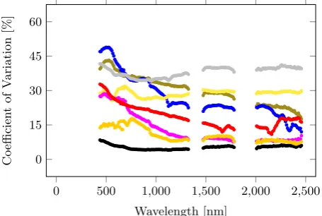
Coefficient of variation is an indicator which one can use to calcu-late the distribution and is expressed as percentage. It is defined by dividing the standard deviation with the mean, as seen in

cv=

σ

µ (2)

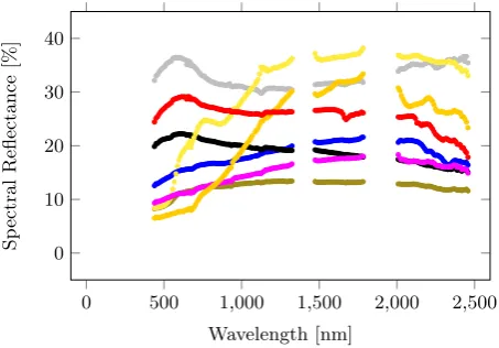
This indicator is in this work used to display the distribution of the spectral reflectance of the classified materials across different wavelengths. Hence, it is possible to determine which parts of the spectral domain contain the most variation. The mean spectra and the coefficient of variation spectra for the classes of the URBAN-SAT dataset can be seen in Figures 3 and 5 and for those of the Santa Barbara dataset in Figures 4 and 6.

0 500 1,000 1,500 2,000 2,500 0

10 20 30 40

Wavelength [nm]

S

p

ec

tra

l

R

efl

ec

ta

n

ce

[%

]

Figure 3. Mean spectra for the URBAN-SAT dataset (Glass: cyan;Concrete: red;Metal: gray;Wood: orange;Fibre Cement: green).

0 500 1,000 1,500 2,000 2,500 0

10 20 30 40

Wavelength [nm]

S

p

ec

tra

l

R

efl

ec

ta

n

ce

[%

]

Figure 4. Mean spectra for the Santa Barbara dataset ( Compos-ite: olive green;Gravel: blue;Metal: gray;Asphalt: black;Tile: yellow;Tar: magenta;Wood: orange;Concrete: red).

In a first experiment, we consider the URBAN-SAT dataset where the reference labeling refers to the five semantic classesGlass, Concrete,Metal,WoodandFibre Cement. We randomly select

(5)

0 500 1,000 1,500 2,000 2,500

Figure 5. Coefficient of variation spectra for the URBAN-SAT dataset (Glass: cyan;Concrete: red;Metal: gray;Wood: orange; Fibre Cement: green).

Figure 6. Coefficient of variation spectra for the Santa Barbara dataset (Composite: olive green;Gravel: blue;Metal: gray; As-phalt: black;Tile: yellow;Tar: magenta;Wood: orange; Con-crete: red).

to noise (i.e. the spectral bands in the range of1351-1440nm,

1798-1957nm and>2400nm). As a consequence, we consider spectral information corresponding to1801spectral bands. Us-ing the reflectance values correspondUs-ing to these channels deliv-ers the feature setS_all,orig_{, applying a PCA yields the feature set} S_all,PCA, and only using the spectral bands selected via CFS re-sults in the feature setSall,CFS. In addition to the original spectra, we separately consider the301spectral bands that correspond to the visible spectrum in the range of400-700nm, which deliv-ers the feature setsS_visible,orig,S_visible,PCAandS_visible,CFS, re-spectively. Furthermore, we separately consider the501spectral bands that correspond to the VNIR spectrum in the range of450

-950nm, which yields the feature setsS_VNIR,orig, S_VNIR,PCA andSVNIR,CFS, respectively. Finally, we consider the1151 spec-tral bands that correspond to the SWIR spectrum in the range of

1000-2400nm when discarding the spectral bands in the range of1351-1440nm and1798-1957nm. This results in the feature setsSSWIR,orig,SSWIR,PCAandSSWIR,CFS. Relying on the12 different feature sets, we perform a standard supervised classifi-cation. The results achieved with the RF classifier and the SVM classifier are provided in Table 1.

In a second experiment, we consider the Santa Barbara dataset where the reference labeling refers to eight semantic classes which were defined by us:Composite,Gravel,Metal,Asphalt,Tile,Tar, Woodand Concrete. On the one hand, we consider the use of

all available spectral information (172spectral bands) after re-moving the bands which are sensitive to noise (i.e. the spectral bands in the range of1325-1473nm and1783-2008nm). On the other hand, we consider the use of only the spectral bands that correspond to the visible spectrum in the range of400-700nm (29spectral bands), the use of only the spectral bands that cor-respond to the VNIR spectrum in the range of450-950nm (53

spectral bands) and the use of the spectral bands that correspond to the SWIR spectrum in the range of1000-2400nm (105 spec-tral bands) after discarding the specspec-tral bands which are sensitive to noise. We therefore obtain12different feature sets in anal-ogy to the first experiment. For classification, we again use a RF classifier and an SVM classifier. The respectively achieved classification results are provided as well in Table 1.

5. DISCUSSION

The main objectives of this work were to classify common ma-terials found on buildings, by using the datasets of Santa Bar-bara and URBAN-SAT and to evaluate the achieved results. The added value of using dimensionality reduction and feature/band selection as well as parts of the full spectra domain were evalu-ated. Hence, by comparing the classification approaches, we have concluded the following.

RF compared to SVM achieves better classification results for both datasets, which can be seen with the better overall accu-racy and higherκ-values. SVM does achieve classification re-sults close to RF when the full spectra domain is used, but not the sub-bands are chosen. Overall, the classification of the materials in the Santa Barbara dataset is superior to the classification of the materials in the SAT dataset. However, the URBAN-SAT dataset compared to the Santa Barbara dataset consists of fewer samples, hence it contains a larger variation of spectra for each material. This is noticeable while studying the provided ta-bles, since the scores using the URBAN-SAT dataset are lower than the scores generated from the Santa Barbara dataset in addi-tion to the generally higher coefficient of variaaddi-tion.

The PCA-based dimensionality reduction achieves in general a higher overall accuracy than CFS and when none of them is used. The scoring also indicates that it is better to use no feature se-lection than to use CFS, since CFS performs in general worse. Additionally, the scores seen in the tables when the full domain is used are the best, followed by using the sub-band of SWIR. The VNIR domain achieves better classification results than the SWIR domain with the URBAN-SAT dataset, with the opposite results for the Santa Barbara dataset. However, the URBAN-SAT dataset contains in comparison to the Santa Barbara dataset more noise in the SWIR domain, which can be seen in Figure 5. Hence, the SWIR domain loses values for classifying materials with the URBAN-SAT dataset. This could indicate that the VNIR domain can be sufficient for material classification.

(6)

Sall Svisible SVNIR SSWIR

orig PCA CFS orig PCA CFS orig PCA CFS orig PCA CFS

OA[%]

URBANSATRF 85.0 87.5 69.8 71.9 81.3 63.1 80.6 83.8 65.0 76.9 75.6 71.3 URBANSATSVM 77.5 76.9 71.3 68.1 68.1 60.0 70.6 69.4 64.4 66.9 65.0 65.6 SantaBarbaraRF 86.0 90.4 85.4 70.3 81.6 67.6 70.6 81.9 71.4 69.0 85.2 62.9 SantaBarbaraSVM 82.4 82.1 83.5 65.6 65.6 65.9 70.1 70.1 71.4 74.5 72.8 69.5

κ[%]

¯ R[%]

¯ P[%]

¯ F1[%]

Table 1. Classification results achieved for the two datasets

Different types of building materials are used in different coun-tries which needs to be kept in mind. In our case, the two datasets have been collected in two different countries. The type of wood which might be use as building material in the Santa Barbara re-gion (USA) may not be the same in the Karlsruhe rere-gion (Ger-many). Therefore, it might not be feasible to compare the spectral reflectance of the same material from the two datasets, since they might not be the same type of material.

6. CONCLUSION AND OUTLOOK

In this work, we have classified building materials using the Santa Barbara dataset and our own dataset URBAN-SAT. Two classifi-cation approaches were used, SVM and RF, in addition to PCA-based dimensionality reduction and CFS-PCA-based feature selection. The classification results indicate that RF is in general better than SVM for the two used datasets, achieving a higher overall accu-racy and higherκ-values. In addition, usage of the PCA-based dimensionality reduction contributes as well to those better clas-sification results. While comparing the three sub-bands, one can tell that the full domain provides the better values, followed by the SWIR and the VNIR domain. However, the results indicate that the VNIR domain is sufficient for material classification.

As future work, we want to significantly extend the URBAN-SAT database by having a larger variation of building materials and increasing the number of acquired samples. A spectral variation caused by small differences in the solar radiation is noticeable, as seen in results in the SWIR domain. URBAN-SAT should therefore contain material samples exposed from different inten-sities of solar radiation (at both cloudy and sunny conditions). This would extend the usage of the library, since the spectral re-flectance is strongly affected by intensity of the solar radiation. In general, laboratory created libraries do not reflect the reality since the data is collected with a constant intensity of solar radi-ation. The level of detail that describes the materials, meaning differencing for example metals, should be on a finer level than the one used in this work for an increased usage.

ACKNOWLEDGEMENT

The authors would like to thank Jens Kern for the support during the acquisition of building materials and the Institute of

Technol-ogy and Management in Construction (TMB) at KIT for letting us collect data at their testing ground. This work is a part of the research cluster URBAN-SAT, a part of the graduate school GRACE.

REFERENCES

Baldridge, A., Hook, S., Grove, C. and Rivera, G., 2009. The ASTER spectral library version 2.0.Remote Sensing of Environ-ment113(4), pp. 711–715.

Breiman, L., 2001. Random forests. Machine Learning45(1), pp. 5–32.

Camps-Valls, G., Tuia, D., Bruzzone, L. and Benediktsson, J. A., 2014. Advances in hyperspectral image classification: Earth monitoring with statistical learning methods. IEEE Signal Pro-cessing Magazine31(1), pp. 45–54.

Chang, C.-C. and Lin, C.-J., 2011. LIBSVM: a library for support vector machines. ACM Transactions on Intelligent Systems and Technology2(3), pp. 27:1–27:27.

Chehata, N., Le Bris, A. and Najjar, S., 2014. Contribution of band selection and fusion for hyperspectral classification. In: Proceedings of the 7th Workshop on Hyperspectral Image and Signal Processing: Evolution in Remote Sensing, pp. 1–4.

Chi, M., Feng, R. and Bruzzone, L., 2008. Classification of hy-perspectral remote-sensing data with primal SVM for small-sized training dataset problem. Advances in Space Research41(11), pp. 1793–1799.

Cochrane, M., 2000. Using vegetation reflectance variability for species level classification of hyperspectral data. International Journal of Remote Sensing21(10), pp. 2075–2087.

Cortes, C. and Vapnik, V., 1995. Support-vector networks. Ma-chine Learning20(3), pp. 273–297.

Criminisi, A. and Shotton, J., 2013.Decision forests for computer vision and medical image analysis. Advances in Computer Vision and Pattern Recognition, Springer, London, UK.

(7)

Guyon, I. and Elisseeff, A., 2003. An introduction to variable and feature selection. Journal of Machine Learning Research3, pp. 1157–1182.

Hall, M. A., 1999. Correlation-based feature subset selection for machine learning. PhD thesis, Department of Computer Science, University of Waikato, New Zealand.

Ham, J., Chen, Y., Crawford, M. M. and Ghosh, J., 2005. In-vestigation of the random forest framework for classification of hyperspectral data. IEEE Transactions on Geoscience and Re-mote Sensing43(3), pp. 492–501.

Heiden, U., Segl, K., Roessner, S. and Kaufmann, H., 2007. De-termination of robust spectral features for identification of urban surface materials in hyperspectral remote sensing data. Remote Sensing of Environment111(4), pp. 537–552.

Herold, M., Gardner, M. and Roberts, D., 2003. Spectral reso-lution requirements for mapping urban areas.IEEE Transactions on Geoscience and Remote Sensing41(9), pp. 1907–1919.

Herold, M., Roberts, D. A., Gardner, M. E. and Dennison, P. E., 2004. Spectrometry for urban area remote sensing - Development and analysis of a spectral library from 350 to 2400 nm. Remote Sensing of Environment91(3), pp. 304–319.

Hughes, G. F., 1968. On the mean accuracy of statistical pattern recognizers. IEEE Transactions on Information Theory14(1), pp. 55–63.

Joelsson, S. R., Benediktsson, J. A. and Sveinsson, J. R., 2005. Random forest classifiers for hyperspectral data. In:Proceedings of the International Geoscience and Remote Sensing Symposium, pp. 160–163.

Keller, S., Braun, A. C., Hinz, S. and Weinmann, M., 2016. In-vestigation of the impact of dimensionality reduction and feature selection on the classification of hyperspectral EnMAP data. In: Proceedings of the 8th Workshop on Hyperspectral Image and Signal Processing: Evolution in Remote Sensing, pp. 1–6.

Keller, S., Braun, A. C., Hinz, S. and Weinmann, M., 2017. Investigation of the potential of hyperspectral EnMAP data for land cover and land use classification. Tagungsband der 37. Wissenschaftlich-Technischen Jahrestagung der DGPF 26, pp. 110–121.

Kotthaus, S., Smith, T. E. L., Wooster, M. and Grimmond, C., 2014. Derivation of an urban materials spectral library through emittance and reflectance spectroscopy. ISPRS Journal of Pho-togrammetry and Remote Sensing94, pp. 194–212.

Kutser, T., Miller, I. and Jupp, D., 2006. Mapping coral reef benthic substrates using hyperspectral space-borne images and spectral libraries. Estuarine, Coastal and Shelf Science70(3), pp. 449–460.

Le Bris, A., Chehata, N., Briottet, X. and Paparoditis, N., 2014. Use intermediate results of wrapper band selection methods: a first step toward the optimization of spectral configuration for land cover classifications. In: Proceedings of the 7th Workshop on Hyperspectral Image and Signal Processing: Evolution in Re-mote Sensing, pp. 1–4.

Le Bris, A., Chehata, N., Briottet, X. and Paparoditis, N., 2016. Spectral band selection for urban material classification using hy-perspectral libraries. ISPRS Annals of Photogrammetry, Remote Sensing and Spatial Information SciencesIII(7), pp. 33–40.

Liaw, A. and Wiener, M., 2002. Classification and regression by randomForest.R News2/3, pp. 18–22.

Licciardi, G., Marpu, P. R., Chanussot, J. and Benediktsson, J. A., 2012. Linear versus nonlinear PCA for the classification of hy-perspectral data based on the extended morphological profiles. IEEE Geoscience and Remote Sensing Letters9(3), pp. 447–451.

Melgani, F. and Bruzzone, L., 2004. Classification of hyper-spectral remote sensing images with support vector machines. IEEE Transactions on Geoscience and Remote Sensing 42(8), pp. 1778–1790.

Plaza, A., Benediktsson, J. A., Boardman, J. W., Brazile, J., Bruz-zone, L., Camps-Valls, G., Chanussot, J., Fauvel, M., Gamba, P., Gualtieri, A., Marconcini, M., Tilton, J. C. and Trianni, G., 2009. Recent advances in techniques for hyperspectral image process-ing.Remote Sensing of Environment113, pp. S110–S122.

Rao, N. R., Garg, P. and Ghosh, S., 2007. Development of an agricultural crops spectral library and classification of crops at cultivar level using hyperspectral data.Precision Agriculture 8(4-5), pp. 173–185.

Saeys, Y., Inza, I. and Larra˜naga, P., 2007. A review of feature selection techniques in bioinformatics. Bioinformatics 23(19), pp. 2507–2517.

Shepherd, K. and Walsh, M., 2002. Development of reflectance spectral libraries for characterization of soil properties. Soil Sci-ence Society of America Journal66(3), pp. 988–998.

Wang, J. and Chang, C.-I., 2006. Independent component analysis-based dimensionality reduction with applications in hy-perspectral image analysis. IEEE Transactions on Geoscience and Remote Sensing44(6), pp. 1586–1600.

Zhao, Z., Morstatter, F., Sharma, S., Alelyani, S., Anand, A. and Liu, H., 2010. Advancing feature selection research – ASU fea-ture selection repository. Technical report, School of Computing, Informatics, and Decision Systems Engineering, Arizona State University, Tempe, AZ, USA.