Welcome to ePrints Sriwijaya University - UNSRI Online Institutional Repository

(1)

institutional repository. Authors requiring further information

regarding Elsevier’s archiving and manuscript policies are

encouraged to visit:

(2)

Seasonal and interannual patterns of sea surface temperature in Banda Sea as

revealed by self-organizing map

Iskhaq Iskandar

1,n

Research Institute for Global Change, Japan Agency for Marine-Earth Science and Technology (JAMSTEC), 2-15, Natsushima, Yokosuka, Kanagawa 237-0061, Japan

a r t i c l e

i n f o

Seasonal and interannual variations of sea surface temperature (SST) in the Banda Sea are studied for the period of January 1985 through December 2007. A neural network pattern recognition approach based on self-organizing map (SOM) has been applied to monthly SST from the Advanced Very High Resolution Radiometer (AVHRR) Oceans Pathfinder. The principal conclusions of this paper are outlined as follows. There are three different patterns associated with the variations in the monsoonal winds: the southeast and northwest monsoon patterns, and the monsoon-break patterns. The southeast monsoon pattern is characterized by low SST due to the prevailing southeasterly winds that drive Ekman upwelling. The northwest monsoon pattern, on the other hand, is one of high SST distributed uniformly in space. The monsoon-break pattern is a transitional pattern between the northwest and southeast monsoon patterns, which is characterized by moderate SST patterns. On interannual time-scale, the SST variations are significantly influenced by the El Ninõ-Southern Oscillation (ENSO) and Indian Ocean Dipole (IOD) phenomena. Low SST is observed during El Ninõ and/or positive IOD events, while high SST appears during La Ninã event. Low SST in the Banda Sea during positive IOD event is induced by upwelling Kelvin waves generated in the equatorial Indian Ocean which propagate along the southern coast of Sumatra and Java before entering the Banda Sea through the Lombok and Ombai Straits as well as through the Timor Passage. On the other hand, during El Ninõ (La Ninã) events, upwelling (downwelling) Rossby waves associated with off-equatorial divergence (convergence) in response to the equatorial westerly (easterly) winds in the Pacific, partly scattered into the Indonesian archipelago which in turn induce cool (warm) SST in the Banda Sea.

1. Introduction

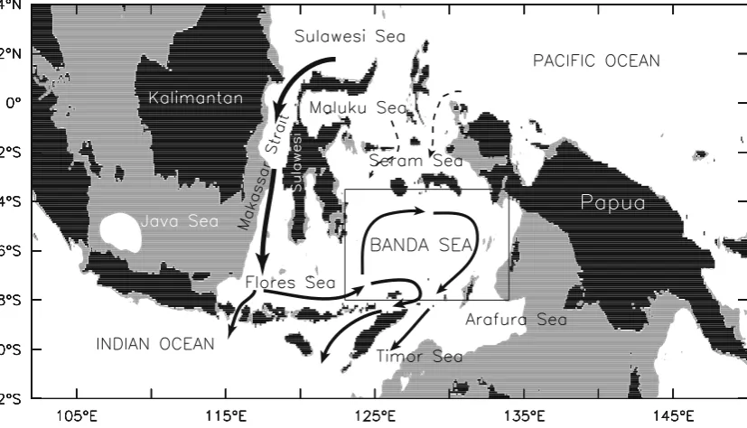
The Banda Sea, outlined by the Southern Molucca islands (i.e. Seram, Sula and Buru islands) on the north and Nusa Tenggara Islands Chain on the south, is located on the route of Indonesian Throughflow (ITF) (Fig. 1). Part of the ITF waters flows through the Banda Sea via Flores Sea in the south and Halmahera and Seram seas in the north, before exiting to the Indian Ocean via Timor Sea and Ombai Strait (Wyrtki, 1961; Gordon and Fine, 1996), and through the Lombok Strait (Wyrtki, 1958; Gordon and Susanto, 2001). The upper part of this throughflow is an element of the global thermohaline circulation which links the Pacific and Indian Ocean (Gordon, 1986). Previous studies have confirmed the importance of this throughflow on the global ocean and climate circulation (Hirst and Godfrey, 1993;Godfrey, 1996; Schneider, 1998;Wajsowicz and Schneider, 2001;Lee et al., 2002).

The ITF water entering the Banda Sea experiences significant transformation. Ffield and Gordon (1992) have suggested that vertical mixing in the Banda Sea is responsible for the transformation of the incoming Pacific water characterized by subsurface salinity maximum into unique ITF water that has low salinity (Ffield and Gordon, 1992). In addition, strong tidal mixing in the Banda Sea enhances the mixing of deep and surface waters leading to the modification of sea surface temperature (SST) in this peculiar sea. This result is consistent with an early study that suggested the role of advection, air-sea flux and seasonal upwelling in controlling SST in the Banda Sea (Wyrtki, 1961). Moreover,Gordon and Susanto (2001)found that seasonal change in SST is associated with the local Ekman upwelling driven by the monsoonal winds. They showed that SST decreases to about 26.51C during the southeast monsoon, while it increases to about 29.51C during the northwest monsoon. Similarly, recent studies have also suggested that the monsoonal winds have a dominant influence on SST variability within the Indonesian seas region (Qu et al., 2005;Susanto et al., 2006;Kida and Richards, 2009).

Moreover, variability of the SST in the Indonesian region, including the Banda Sea, has shown to have an important role on climate variations in the Indo-Paciﬁc sector, with important Contents lists available atScienceDirect

journal homepage:www.elsevier.com/locate/csr

Continental Shelf Research

n

Current address: NOAA/PMEL, 7600 Sand Point Way NE, Seattle, WA 98115, USA. Tel.:+ 1 206 526 6885; fax: + 1 206 526 6744.

E-mail address:Iskhaq.Iskandar@noaa.gov

1

(3)

consequences for global climate (Qu et al., 2005). Climate-model experiments show that precipitation over the western Paciﬁc and western Indian Oceans is very sensitive to the SST variations in the Indonesian seas (Qu et al., 2005). Recent study has shown a robust correlation between SST and precipitation over the Maritime Continent (Dayem et al., 2007). High precipitation rates over the Maritime Continent are associated with high SST. They also suggested that the strength of the Walker Circulation is related to the precipitation rates over the Maritime Continent. When the precipitation increases, the surface easterlies over the tropical Paciﬁc Ocean are strengthened leading to a strong Walker Circulation.

Understanding the SST variations in the Indonesian seas, including the Banda Sea, is critical for understanding tropical climate variability. However, study of the SST variability in this region within a season, from season to season and year to year is hindered by the dearth of in-situ observations. One of available SST data in this region which have high spatial resolution and long heritage (more than 20 years) is from the thermal infrared SST measurement of Advanced Very High Resolution Radiometer (AVHRR). This measurement, however, is sensitive to the presence of cloud leading to uneven data in time and space, in particular in the tropical ocean that is often covered by cloud. Taking advantage of one particular method that has proved useful in this respect so-calledself-organizing map(SOM), this study further exploits the satellite-retrieved SST variations in the Banda Sea.

The SOM is one type of unsupervised Artiﬁcial Neural Network (ANN) that is mainly used for pattern recognition and classiﬁca-tion (Kohonen et al., 1995; Kohonen, 2001). It is a nonlinear, ordered, smooth mapping of high-dimensional input data onto the elements of regular, low-dimensional array. The SOM has been applied widely to climate and meteorology (e.g. Hewitson

and Crane, 2002; Cavazos, 2000; Hong et al., 2004) and

oceanography (Richardson et al., 2003;Liu and Weisberg, 2005; Liu et al., 2006a;Cheng and Wilson, 2006;Iskandar et al., 2008; Tozuka et al., 2008). All these studies suggested that the SOM is a powerful tool for identifying patterns of continuous, dynamic processes in complex data sets.

The remainder of this paper is organized as follows. A brief description of the data and method used in this study is given in

the next section. In Section 3, the seasonal and interannual variations of SST in Banda Sea are analyzed using the SOM. In particular, relationship between SST in the Banda Sea and ENSO as well as Indian Ocean Dipole/IOD (Saji et al., 1999;Webster et al., 1999; Murtugudde et al., 2000) phenomena is also discussed in this section. Finally, discussion and summary are given in the last section.

2. Data and method of analysis

2.1. Data

Monthly SST data set from the NODC/RSMAS AVHRR Oceans Pathﬁnder version 5.0 is used in the present study. The data cover the period from January 1985 to December 2007 with horizontal resolution of 4 km. The SST data have been prepared by calculating average in 0.2510.251 boxes between 1231E to 1341E and 81S to 3.51N (seeFig. 1a). The land was removed from the analysis, so that the input data consists of 808 sea pixels. The ﬁnal input matrix consists of 808 columns (pixels)276 rows (months).

In order to explain the dynamics underlying the SST variations in the Banda Sea, monthly sea surface height (SSH) data with horizontal resolution of 1/311/31from the Archiving, Validation and Interpretation of Satellite Oceanography(AVISO) are used. In addition, the monthly winds from NCEP/NCAR reanalysis with spatial resolution of 2.51 are also used to estimate the Ekman upwelling and downwelling.

2.2. Self-organizing map (SOM)

Since the SOM is relatively new to oceanography, a brief description of the method is given here. Prior to the analysis, the input data are arranged into two-dimensional array with dimen-sions equal tonumber of pixels per time stepnumber of time steps. The SOM is then initiated by deﬁning the shape and dimension of the SOM array, which depends on the complexity of the studied problem and the level of details desired in the analysis. In this

(4)

study, several dimensions of the SOM array have been tested to find the most sufficient array that covers the original data space. It is found that a 34 SOM array is sufficient to describe the SST variability in the Banda Sea. Note that each nodei in the SOM array is associated with a weight vector,_w

ithat may be initialized randomly and its dimension is equal to that of the input vector,_x_.

The training process starts by presenting the ﬁrst input vector to the SOM, and the activation of each unit for the presented input vector is calculated using an activation function, which is Euclidian distance between the weight vector of the unit and the input vector. The node responding maximally to a given input vector (i.e. the smallest Euclidian distance) is selected to be the ‘‘winner’’ or the Best-Matching Unit (BMU)ck:

ck¼arg min:!xk,wi: ð1Þ

where ‘‘arg’’ denotes index,,_x

kindicates the present input vector and

,_w

i is the weight vector. The weight vector of thewinneris moved towards the presented input vector by a certain fraction of the Euclidean distance as shown by a time-decreasing learning rate

a

. In this study, a linear time function is used for the learning rate

a

ðtÞ ¼

a

₀ð1t=TÞ ð2Þ

where

a

0 is the initial learning rate and T signiﬁes the length of training.

The weight vectors of units in the neighborhood of thewinner are also modiﬁed according to a spatial-temporal neighborhood function

e

. The neighborhood function

e

also shrinks over time

and decreases spatially away from thewinner. There are two types of the neighborhood function available in the software; bubble

and Gaussian functions. Liu et al. (2006b) have conducted a

performance evolution of the SOM using patterns of a linear progressive sine wave. Their study has shown that the bubble function gives more accurate SOM patterns than the Gaussian function. In this study, therefore, abubblefunction is used for the neighborhood function

e

ðtÞ ¼Fð

s

_tdciÞ ð3Þ

where

s

_tis the neighborhood radius that also linearly decreases

between the initial and the ﬁnal step,dciis the distance between a node and thewinnernode.Fis a step function and it is deﬁned as:

FðxÞ ¼ 0 if x

o0 1 if xZ0:

(

ð4Þ

The learning rule, then, is deﬁned as

,_w

iðtþ1Þ ¼,wiðtÞ þ

a

ðtÞ

e

ðtÞ ,xðtÞ,wiðtÞ

n o

, ð5Þ

wheretdenotes the current learning iteration and,_x_{indicates the}

currently presented input vector.

The training is performed in two phases. The ﬁrst phase had a learning rate of 0.5, an initial update radius of 4 and a training length of 200 cycles. Then, the second phase had a learning rate of 0.1, an initial update radius of 1 and a training length of 500 cycles. After these training processes, the SOM array consists of a number of patterns characteristic of the input data, with similar patterns are mapped onto neighboring regions on the SOM array, while dissimilar patterns are mapped farther apart.

3. Results

3.1. Seasonal variability from monthly mean climatology

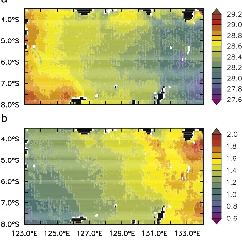
Before calculating the monthly mean climatology, we ﬁrst show the time mean (1985–2007) and standard deviation of the observed SST in the Banda Sea (Fig. 2). It is shown that the time-mean SST reveals a clear east–west SST gradient with maximum value in the

western Banda Sea, decreasing eastward (Fig. 2a). The coldest SST values are observed near the western coast of Papua, while warm water is found in the southwestern Banda Sea near the Flores Sea. On the other hand, the standard deviation ﬁeld (Fig. 2b) indicates that the greatest SST variation is found in the eastern Banda Sea, as previously described byGordon and Susanto (2001).

Gordon and Susanto (2001)have calculated the area-averaged climatological monthly SST from the weekly optimal interpolation SST analysis (Reynolds and Smith, 1994) during 1982–2000. It is, then, useful to calculate the climatological monthly SST maps and to compare the results with those obtained by Gordon and Susanto (2001)to see whether the results reveal new features, in particular the spatial patterns of the seasonal SST variation.

General feature of the climatological monthly SST maps is similar to that found by Gordon and Susanto (2001), which shows two prominent patterns of the SST variations (Fig. 3). The ﬁrst pattern shows that the Banda Sea have a period of warm SST (4291C) lasting during the northwest monsoon from November through April. Note that the climatological monthly SST maps show that the warm period is characterized by a roughly uniform SST throughout the basin, though a slight cooling event is observed in the southeastern basin near the Flores Sea during February. The second pattern observed during June–September exhibits low SST in the Banda Sea. This low SST pattern is characterized by a strong SST gradient with colder SST near the eastern boundary of the basin. A minimum SST of about 251C is observed in August at the northeast and southeast corners of the basin.

Previous studies have suggested that seasonal variation of the monsoonal winds is a dominant forcing for the seasonal SST variations in the Banda Sea (Wyrtki, 1961;Gordon and Susanto, 2001). In particular,Wyrtki (1961)proposed that coastal upwel-ling driven by southeasterly winds is responsible for the cool SST during the southeast monsoon. Moreover,Gordon and Susanto (2001)suggested that Ekman upwelling associated with south-easterly winds is a driving force for the low SST in the Banda Sea. More recently, using a regional ocean model,Kida and Richards (2009)investigated in more detail the mechanism of seasonal SST variability in the eastern Indonesian seas, e.g. Banda and Arafura

Fig. 2.(a) 23-year mean and (b) standard deviation of sea surface temperature in

(5)

seas. They suggested that seasonal SST variability in the eastern Indonesian seas is mostly controlled by the monsoonal winds. Moreover, they found that about half of basin-averaged SST variability is forced by the winds, while the remaining is controlled by the heat ﬂuxes in the surface. An important result from their study is related to the strong SST gradient during the southeast monsoon. They suggested that both southeasterly winds and a unique bathymetry of the eastern Indonesian seas cause the SST gradient. During this season, the winds generate upwelling (downwelling) in the northern (southern) basin. Strong upwelling in the northeastern basin where the bathymetry is shallow enhances the SST cooling through the mixing of

subsurface water with the warm surface water. In addition, the presence of shallow region in the eastern basin prevents the advection of warm water from the western basin.

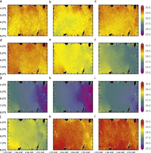
3.2. Seasonal variability from 34 SOM results

The 34 SOM array representing the SST variations in the Banda Sea is shown inFig. 4. This SOM array has been arranged in such a way that similar SST patterns are located adjacent to one another, while dissimilar patterns are located farther away from each other. Each map represents a typical SST patterns within the

(6)

original data, which is constructed from the weights on that particular node. Note that the total number of the SOM patterns is similar to that from monthly mean climatology, so that results from the SOM analysis can be compared with those from the climatological analysis. This comparison may provide new insights into the seasonal SST variations in the Banda Sea, which are captured by the SOM analysis.

Generally, low SST patterns are located on the top-two rows of the SOM array, while high SST patterns are distributed in the bottom row of the SOM array. The transitional patterns char-acterized by moderate SST patterns are located in the third row of the SOM array. Also, there is remarkable difference between node

1 and node 12. In node 1, low SST covers the Banda Sea especially in the eastern part. In contrast, high SST covers most of the Banda Sea region in node 12.

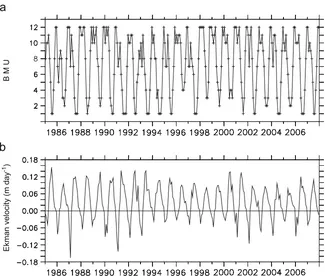
The temporal evolution of those spatial SST patterns is expressed in the BMU time series (Fig. 5a). The BMU indicates that the SST patterns in the Banda Sea have both seasonal and interannual pattern. Generally, the seasonal variation indicated by the BMU shows that the northwest monsoon is characterized by nodes 10–12, while the southeast monsoon is dominated by nodes 1–4. This seasonal variation is in a good agreement with the seasonal variation of the winds (Fig. 5b). It is clearly shown that the downwelling (upwelling) favorable winds during the

(7)

northwest (southeast) monsoon induce Ekman convergence (divergence).

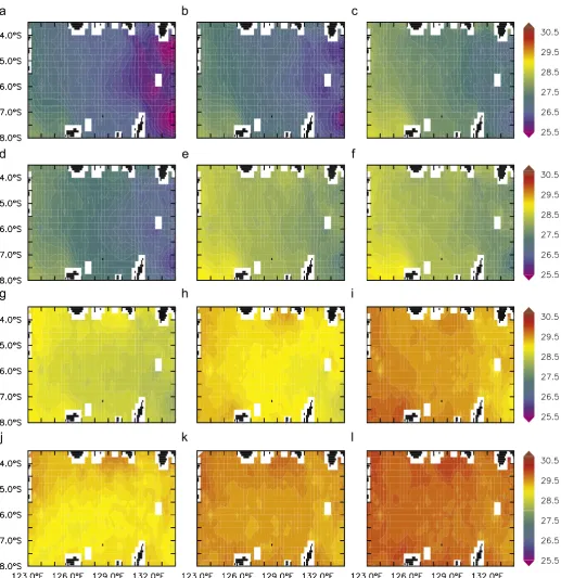
To further evaluate the seasonal variation, monthly frequency maps of the 34 SOM are calculated (Fig. 6). These maps indicate how frequent each particular node in the SOM array appears in the original data. It is shown that during the northwest monsoon from November through April, high SST patterns located in the bottom row of the SOM array appear more frequently on the monthly frequency maps. Node 12 mostly occurs during November and December. In January, nodes 10 and 12 dominate the SST pattern, while node 10 and 7 mainly appear in February. Node 11 appears mostly from March to April, with peak frequency of occurrence in March.

On the other hand, the most frequent pattern during the southeast monsoon from June through September is the top row nodes in the SOM array, which are characterized by low SST patterns. Node 3 occurs mostly during June, while node 1 mainly appears from July through August with peak frequency of occurrence in August. In September, nodes 1, 3 and 4 dominate the SST pattern in the SOM array. The May and October patterns are the transition between the northwest and southeast mon-soons, which are populated mostly by node 8 and node 7, respectively. This transition pattern is characterized by moderate SST patterns. As a whole, the seasonal variability of the SST in Banda Sea obtained from the SOM analysis can be deﬁned into three categories: (1) southeast monsoon pattern which is populated by nodes 1 through 6, (2) northwest monsoon pattern which is populated by nodes 9 through 12, and (3) transition pattern which is characterized by moderate SST pattern in nodes 7 and 8. This result is in good agreement with that obtained from monthly mean climatological analysis (seeFig. 3). Thus, we may suggest that the SOM is successful in detecting the seasonal variation of the SST in the Banda Sea.

In addition, it should be noted that the SOM method is a nonlinear analysis based on the iterative learning process. The resulting SOM array from this analysis is not a simple average of

data as in the monthly climatology. Therefore, it may suggest that the seasonal patterns reproducing from the SOM analysis are more accurate than the monthly mean maps. As shown inFigs. 5a and 6, one particular pattern may be found in several months, while the other may appear just in one month. Thus, each pattern of the SOM has different frequency of occurrence. For example, pattern 12 characterized by high SST can be seen in November and December, while the monthly climatology of the SST only shows that this pattern only appear in December.

3.3. Interannual variation and its relation to ENSO and indian ocean dipole

As shown by the BMU time series (Fig. 5a), the SST patterns in the Banda Sea also exhibit interannual variations. In order to evaluate the interannual variations of the SST in Banda Sea, annual frequency maps for each annual cycle from April to March of the following year are calculated. The maps are constructed by calculating the number of month mapped to each node in the SOM array. Note that the deﬁnition of the annual cycle is designed to capture the occurrence of both ENSO and IOD events.

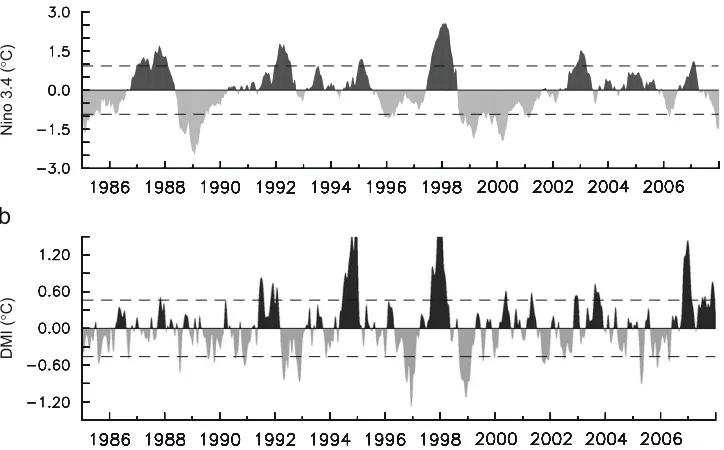
Fig. 7shows the annual frequency maps for La Nin˜ a years in 1988/89 and 1998/99, El Nin˜ o years in 1986/97, 1991/92 and 2002/03, IOD years in 1994 and 2006, and El Nin˜ o co-occurred with IOD in 1997/98. The deﬁnition of ENSO and IOD years is based on the Nin˜ o-3.4 index and Dipole Mode Index (DMI), respectively (Fig. 8). The Nin˜ o-3.4 index is computed from monthly SST anomaly (SSTA) in the region 51N–51S, 1201– 1701W. Positive anomalies larger than one standard deviation indicate El Nin˜ o events, and negative anomalies smaller than one standard deviation indicates La Nin˜ a events. On the other hand, the DMI is deﬁned as the SSTA difference between the western equatorial Indian Ocean (501E–701E, 101S–101N) and the eastern equatorial Indian Ocean (901E–1101E, 101S–equator) (Saji et al.,

B M U

Ekman velocity (m day

-1)

Fig. 5. Time series of (a) the best-matching unit (BMU) for the twelve SOM patterns shown inFig. 4, (b) Ekman velocity averaged over the Banda Sea. Note that positive

(8)

1999). Positive DMI larger than one standard deviation refers to positive IOD event, while negative IOD event is represented by negative DMI smaller than one standard deviation. Note that the ENSO events is defined when the Ninõ3.4 index exceeds its one standard deviation for at least 4 consecutive months (Trenberth, 1997), while the IOD events is defined if the DMI exceeds its one standard deviation for at least 3 consecutive months (Saji et al., 1999). It is shown that during the La Nin˜ a event in 1988/89 and 1998/ 99, the SOM array is mostly populated by node 12, which is associated with high SST (Fig. 7a–b;see alsoFig. 4). On the other hand, though each El Nin˜ o event indicates different nodal patterns, the annual frequency maps (Fig. 7c and d) shows that the El Nin˜ o events are mostly dominated by node 1 (negative SSHA). An exception is during the 2002/03 El Nin˜ o event where nodes 2 and 3 dominate the SST pattern in the Banda Sea (Fig. 7e, see alsoFig. 4). These results are consistent with the previous findings of Gordon and Susanto (2001). They attributed the

interannual variations of the SST in Banda Sea to the ﬂuctuation of thermocline depth in respond to the remote forcing associated with the ENSO dynamics.

Interesting features captured by the SOM analysis are associated with the IOD event. During IOD event in 1994 and 2006, the Banda Sea experiences cooling event as the SOM array is mostly populated by node 1 (Fig. 7f and g, see alsoFig. 4). In 1997/ 98 when the IOD co-occurred with the El Nin˜o event, the SST in the Banda Sea is characterized by the low SST as expected (Fig. 7h). These results suggest that the IOD event also can have a signiﬁcant impact on the interannual SST variations in the Banda Sea, which is associated with low SST.

Note that the difference in nodal patterns for each particular El Nin˜ o and IOD events can be attributed to the definition of the annual frequency maps, which is from April to March of the following year. Using this definition, during the El Ninõ events we may observe a relatively warm SSTA, which typically occur during

Fig. 6.Monthly frequency maps (%), showing the frequency that SOM patterns identiﬁed inFig. 4occurred for each month. Note that the coordinates correspond to those of

(9)

April. Similarly, during the IOD events, we may also ﬁnd warm SSTA after the termination of the event in January–March. This is the reason why we still have warm SSTA pattern during both El Nin˜ o and IOD events.

During the 2002/03 El Nin˜ o event, although the annual frequency maps do not show the occurrence of node 1, this typical event is still dominated by the negative SSTA pattern indicated by nodes 2 and 3. It should be noted that the 2002/03

Fig. 7. The annual frequency maps (%) of the SSTA in the Banda Sea. (a–b) during La Nin˜a event, (c–e) during El Nin˜o event, (f–g) during IOD event, and (h) during El Nin˜ o which co-occurred with IOD event. Note that the coordinates correspond to those ofFig. 4and percentages in each year sum to 100: (a) La Nina 1988/1989; (b) La Nina 1998/1999(c) EI Nino 1986/1987(d) EI Nino 1991/1992(e) EI Nino 2002/2003(f) IOD 1994; (g) IOD 2006; (h) EI Nino 1997/98

(10)

(11)

(12)

characterized by almost similar patterns (Fig. 7f and g), while the El Nin˜o events have different patterns from event to event (Fig. 7c–e). On the other hand, when the El Nin˜o co-occurred with the IOD

event, the SST pattern in the Banda Sea indicates a similar pattern with that of the IOD pattern (Fig. 7h). However, it is difﬁcult to show with conﬁdence the dominant forcing for the interannual SST

(13)

Seasonal and interannual variations of SST in Banda Sea are examined with SOM analysis using the observed SST data set from AVHRR Oceans Pathﬁnder version 5.0 for the period of January 1985 through December 2007. A 34 SOM array reveals characteristic of seasonal and interannual SST patterns in the Banda Sea.

At seasonal cycle, the SOM results can be categorized into three different patterns associated with the variations in the monsoonal winds: the southeast and northwest monsoon pat-terns, and the monsoon-break patterns. The southeast monsoon pattern is characterized by low SST due to the prevailing southeasterly winds that drive Ekman upwelling from June through September. The northwest monsoon pattern, on the other hand, is one of high SST distributed uniformly in space which reveals from November through April. The monsoon-break pattern, which appears during May and October, is a transitional pattern between the northwest and southeast monsoon patterns. This pattern is characterized by moderate SST, which is roughly distributed throughout the basin.

On interannual time-scale, the SST patterns in the Banda Sea can be defined into two composite categories: La Nin˜ a pattern and El Nin˜ o and/or IOD pattern. The La Ninã pattern is characterized by high SST, while the El Ninõ and/or IOD pattern is associated with low SST.

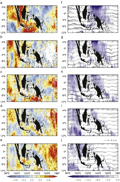
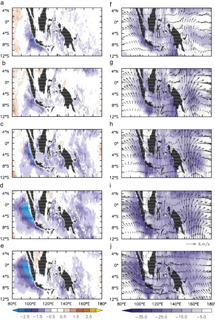
The dynamics underlying the interannual SST variation in the Banda Sea is still an open question.Gordon and Susanto (2001) proposed that the interannual variation of SST in the Banda Sea is due to thermocline fluctuations associated with ENSO dynamics. Previous studies have suggested the importance of remote forcing from the Pacific and the Indian Oceans on the dynamics of the Banda Sea (Wijffels and Meyers, 2004;McClean et al., 2005). This study shows that the interannual SST variations in the Banda Sea are associated with the dynamics of wind-forced equatorial Kelvin and Rossby waves whose signals reached the Banda Sea. Fig. 9 shows the evolution of SSTA, SSH and wind anomalies during El Nin˜ o event in 2002/2003. It is shown that upwelling off-equatorial Rossby waves associated with the off-off-equatorial divergence generated by the westerly winds along the equatorial Pacific Ocean propagate westward. After reaching the eastern coast of Papua, part of these upwelling Rossby waves reflected back into equatorial waveguide and partially scattered into the Indonesian archipelago as coastally trapped waves (CTW). These upwelling CTW in turn cool SST in the Banda Sea. The situations reverse for the La Nin˜ a event (not shown).

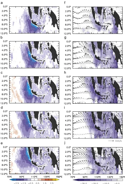
The equatorial Indian Ocean Kelvin waves have also been suggested to penetrate into the Indonesian Seas as far as Makassar Strait and the western Banda Sea (Sprintall et al., 2000;McClean et al., 2005). Moreover, this study shows a unique feature of the SST patterns in the Banda Sea associated with the IOD event. As shown inFig. 10, in June 1994 upwelling Kelvin waves generated by the anomalous easterly winds propagate southeastward along the coastal waveguide. These upwelling Kelvin waves propagates further eastward and then penetrates into Indonesian Seas through the Lombok and Ombai Straits as well as the Timor Passage by July, which then cool SST in the Banda Sea.

When the IOD co-occurred with the El Nin˜ o event, the SST in the Banda Sea is affected by the signal from both the Indian and Paciﬁc region (Fig. 11). In the Indian Ocean site, the upwelling coastal Kelvin waves generated by the easterly winds propagate along the coastal waveguide and then penetrate into the Banda

associated with IOD and El Nin˜ o events. The former is character-ized by almost similar SST patterns from event to event, while the later has different pattern for each event. On the other hand, when the El Nin˜ o co-occurred with the IOD event, the SST pattern in the Banda Sea indicates a similar pattern with that of the IOD pattern. Another forcing mechanism that may lead to the interannual SST variation in the Banda Sea is advection of Paciﬁc warm pool water by the Indonesian Throughﬂow (ITF). Strong ITF is observed during La Nin˜ a event (Meyers, 1996), which is likely to create a warm SST in the Banda Sea. However, this mechanism may not work during El Nin˜ o event as the ITF is weakened.

Acknowledgments:

The author would like to thank Dr. Tomoki Tozuka of the University of Tokyo for helpful discussion on the SOM analysis. The SOM_PAK was prepared by the SOM Programming Team of the Helsinki University of Technology, Finland. The author is grateful to the Japan Society for the Promotion of Science (JSPS) for the ﬁnancial support through a postdoctoral fellowship for foreign researcher. Detailed constructive criticisms and comments from two anonymous reviewers improved the manuscript.

References

Cavazos, T., 2000. Using self-organizing maps to investigate extreme climate events: an application to wintertime precipitation in the Balkans. J. Clim. 13, 1718–1732.

Cheng, P., Wilson, R.E., 2006. Temporal variability of vertical nontidal circulation pattern in a partially mixed estuary: comparison of self-organizing map and empirical orthogonal functions. J. Geophys. Res. 111, C12021, doi:10.1029/ 2005JC003241.

Dayem, K.E., Noone, D.C., Molnar, P., 2007. Tropical western Paciﬁc warm pool and maritime continent precipitation rates and their contrasting relation-ships with the Walker Circulation. J. Geophys. Res. 112, D0601, doi:10.1029/ 2006JC007870.

Fﬁeld, A., Gordon, A.L., 1992. Vertical mixing in the Indonesian thermocline. J. Phys. Oceanogr. 22, 184–195.

Godfrey, J.S., 1996. The effect of the Indonesian Throughﬂow on ocean circulation and heat exchange with the atmosphere: a review. J. Geophys. Res. 101 (C5), 12217–12238.

Gordon, A.L., 1986. Interocean exchange of thermocline water. J. Geophys. Res. 91, 5037–5046.

Gordon, A.L., Fine, R.A., 1996. Pathways of water between the Paciﬁc and Indian oceans in the Indonesian seas. Nature 379, 146–149.

Gordon, A.L., Susanto, R.D., 2001. Banda Sea surface-layer convergence. Clim. Dyn. 52, 2–10.

Hewitson, B.C., Crane, R.G., 2002. Self-organizing maps: application to synoptic climatology. Clim. Res. 22, 13–26.

Hirst, A.C., Godfrey, J.S., 1993. The role of the Indonesian throughﬂow in a global ocean GCM. J. Phys. Oceanogr. 23, 1057–1086.

Hong, Y., Hsu, K., Sorooshian, S., Gao, X., 2004. Precipitation estimation from remotely sensed imagery using an artiﬁcal neural network cloud classiﬁcation system. J. Appl. Meteorol. 43, 1834–1853.

Iskandar, I., Tozuka, T., Masumoto, Y., Yamagata, T., 2008. Impact of Indian Ocean Dipole on instraseasonal zonal currents at 901E on the equator as revealed by self-organizing map. Geophys. Res. Lett. 35, L14S03, doi:10.1029/ 2008GL033468.

Kida, S., Richards, K.J., 2009. Seasonal sea surface temperature variability in the Indonesian seas. J. Geophys. Res. 114, C06016, doi:10.1029/ 2008JC005150.

Kohonen, T., Hynninen, J., Kangas, J., Laaksonen, J., 1995. SOM_PAK, The self-organizing map program package version 3.1, Laboratory of Computer and Information Science. Helsinki University of Technology, Finland 27pp. Kohonen, T., 2001. Self-Organizing Maps 3rd edn. Springer-Verlag, Berlin,

Heidelberg, New York 501pp.

(14)

Liu, Y., Weisberg, R.H., 2005. Patterns of ocean current variability on the West Florida Shelf using the self-organizing map. J. Geophys. Res. 110, C06003, doi:10.1029/2004JC002786.

Liu, Y., Weisberg, R.H., He, R., 2006a. Sea surface temperature patterns on the West Florida Shelf using the Growing Hierarchical Self-Organizing Maps. J. Atmos. Oceanic Technol. 23 (2), 235–338.

Liu, Y., Weisberg, R.H., Mooers, C.N.K., 2006b. Performance evaluation of the self-organizing map for feature extraction. J. Geophys. Res. 111, C05018, doi:10.1029/2005JC003117.

McClean, J. L., Ivanova, D. P., Sprintall, J., 2005. Remote origins of interannual variability in the Indonesian Throughﬂow region from data and a global Parallel Ocean Program simulation, J. Geophys. Res., 110, C10013, 10.1029/ 2004JC002477.

McPhaden, M.J., 2004. Evolution of the 2002 – 2003 El Nin˜o. Bull. Am. Meteor. Soc. 85, 677–695.

Meyers, G., 1996. Variation of Indonesian Throughﬂow and the El Nin˜ o – Southern Oscillation. J. Geophys. Res. 101, 12,255–12,263.

Murtugudde, R., McCreary, J.P., Busalacchi, A.J., 2000. Oceanic processes associated with anomalous events in the Indian Ocean with relevance to 1997–1998. J. Geophys. Res. 105, 3295–3306.

Qu, T., Du, Y., Strachan, J., Meyers, G., Slingo, J., 2005. Sea surface temperature and its variability in the Indonesian region. Oceanography 18, 50–61.

Reynold, R.W., Smith, T.M., 1994. Improved global sea surface temperature analyses. J. Clim. 7, 929948.

Richardson, A.J., Risien, C., Shillington, F.A., 2003. Using self-organizing maps to identify patterns in satellite imagery. Prog. Oceanogr. 59, 223–239.

Saji, N.H., Goswami, B.N., Vinayachandran, P.N., Yamagata, T., 1999. A dipole mode in the tropical Indian Ocean. Nature 401, 360–363.

Schneider, N., 1998. The Indonesian Throughﬂow and the global climate system. J. Clim. 11, 676–689.

Sprintall, J., Gordon, A.L., Murtugudde, R., Susanto, R.D., 2000. A semiannual Indian Ocean forced Kelvin wave observed in the Indonesian seas in May 1997. J. Geophys. Res. 105, 17,217–17,230.

Susanto, D., Moore, T., Marra, J., 2006. Ocean color variability in the Indonesian Seas during the SeaWiFS era, Geochem. Geophys. Geosys. 7, Q05021, doi:10.1029/2005GC001009.

Tozuka, T., Luo, J.J., Masson, S., Yamagata, T., 2008. Tropical Indian Ocean variability revealed by self-organizing maps. Clim. Dyn. 31, 333–343. Trenberth, K.E., 1997. The deﬁnition of El Nin˜o. Bull. Am. Meteor. Soc. 78,

2,771–2,777.

Wajsowicz, R.C., Schneider, E.K., 2001. The Indonesian Throughﬂow’s effect on global climate determined from the COLA Coupled Climate System. J. Clim. 14, 3029–3042.

Webster, P.J., Moore, A.M., Loschnigg, J.P., Leben, R.R., 1999. Coupled ocean-atmosphere dynamics in the Indian Ocean during 1997–1998. Nature 401, 356–360. Wijffels, S., Meyers, G., 2004. An intersection of oceanic wave guides: variability in

the Indonesian Throughﬂow region. J. Phys. Oceanogr. 34, 1232–1263. Wyrtki, K., 1958. The water exchange between the Paciﬁc and the Indian Oceans in

relation to upwelling processes. Inst. Mar. Res., Djakarta. Proc. Ninth Pac. Sci. Congr. 16, 61–65.