Why was the 2008 Indian Ocean Dipole a Short-lived Event?
Iskhaq Iskandar
1,2*, Muhammad Irfan
1, and Fadli Saymsuddin
31
Department of Physics, Faculty of Mathematics and Natural Sciences, University of Sriwijaya, Inderalaya, South Sumatra, Indonesia
2
Center for Geohazard and Climate Change Study, Faculty of Mathematics and Natural Sciences, University of Sriwijaya, Inderalaya, South Sumatra, Indonesia
3
Agency for the Assessment and Application of Technology, Jakarta, Indonesia
Received 26 July 2012; Revised 5 November 2012; Accepted 27 March 2013 KSO, KIOST and Springer 2013
Abstract−In this paper, the role of equatorial oceanic waves in affecting the evolution of the 2008 positive Indian Ocean Dipole (IOD) event was evaluated using available observations and output from a quasi-analytical linear wave model. It was found that the 2008 positive IOD was an early matured and abruptly terminated event: developed in April, matured in July, and diminished in September. During the development and the maturation of the 2008 positive IOD event, the wind-forced Rossby waves played a dominant role in generating zonal current anomalies in the western equatorial Indian Ocean, while a complex interplay between the wind-forced upwelling Kelvin waves and the eastern-boundary-generated Rossby waves accounted for most of the variability in the eastern basin. The latter induced eastward zonal current anomalies near the eastern boundary during the peak phase of the event. The 2008 positive IOD event was abruptly terminated in mid-July. We found that there were strong eastward zonal currents in mid-July, though the surface wind anomalies in the eastern basin continued to be westward (upwelling favorable). Our analysis shows that these eastward zonal currents mainly resulted from the eastern-boundary-generated upwelling Rossby waves, although the contribution from the wind-forced downwelling Kelvin waves was not negligible. These eastward zonal currents terminated the zonal heat advection and provided a favorable condition for surface heat flux to warm the eastern basin.
Key words−equatorial wave, Indian Ocean Dipole, Kelvin waves, Rossby wave
1. Introduction
Indian Ocean Dipole (IOD) is one of the dominant modes of inter-annual climate variability in the tropical Indian
Ocean. A classical positive IOD event is associated with anomalously cold sea surface temperature (SST) occurring in the southeastern tropical Indian Ocean and warm SST anomaly in its western counterpart (Saji et al. 1999; Webster et al. 1999; Murtugudde et al. 2000). Associated with this typical SST pattern, the atmospheric convection over the eastern Indian Ocean warm pool is suppressed, while that off East Africa and the central Indian Ocean is enhanced. This condition leads to excess rainfall over east Africa, India, and some parts of South Asia, while severe drought occurs over the Indonesian region and Australia (Yamagata et al. 2004). Unlike ENSO in the Pacific, however, the IOD is shorter lived and seasonally phase locked to a seasonal cycle, and the peak strength mostly occurs during the boreal fall season.
It has been suggested that the IOD develops through a feedback between zonal wind stress, SST, and thermocline depth anomalies (Saji et al. 1999; Webster et al. 1999). Ocean dynamics play an important role in the evolution of the life cycle of the IOD. Upwelling equatorial Kelvin waves generated by easterly anomalies lift the thermocline in the eastern Indian Ocean, and anomalous southeasterly winds along the coast of Sumatra enhance the cooling in the eastern Indian Ocean (Murtugudde et al. 2000). In the western Indian Ocean, early studies have demonstrated that downwelling off-equatorial Rossby waves associated with an easterly wind anomaly could deepen thermocline and induce warm SST in the western Indian Ocean (Chambers et al. 1999; Rao et al. 2002; Feng and Meyers 2003). In addition, Murtugudde et al. (2000) have also suggested that weakening of the
*Corresponding author. E-mail: [email protected]
southwest monsoon could enhance warming in the western Indian Ocean.
Previous studies have shown that equatorial waves (Kelvin and Rossby waves) play an important role in the evolution of SST anomalies in the equatorial Indian Ocean during IOD events (Chamber et al. 1999; Webster et al. 1999; Vinayachandran et al. 1999; Rao et al. 2002; Feng and Meyers 2003; Rao and Yamagata 2004; Yuan and Liu 2009). In particular, easterly wind anomalies during a positive IOD event generate anomalous upwelling that propagates eastward along the equator as a Kelvin wave, shoaling (deepening) the thermocline in the eastern (western) basin. The same pattern of anomalous wind stress that generates upwelling along the equator gives rise to sea level anomalies off the equator that propagate westward as Rossby waves. In addition, early observational (Reppin et al. 1999; Horii et al. 2008) and numerical (Vinayachandran et al. 1999, 2007; Murtugudde et al. 2000; Nagura and McPhaden 2010b) studies have also reported the change in upper ocean circulation during the IOD events. Basically, the climatological upper-ocean circulation along the equatorial Indian Ocean reveals semi-annual eastward equatorial jets (Wyrtki 1973). This jet is a result of the upper ocean responses to westerly wind bursts during the monsoon transition periods in April/May and October/November. However, the westerly winds are absent during positive IOD events leading to the weakening or even the reversal of the eastward equatorial jet during boreal fall.
The role of equatorial waves in the termination of the IOD events is also well documented (Rao and Yamagata 2004; Yuan and Liu 2009). Using multi-satellite observations, Rao and Yamagata (2004) proposed that most IOD events were terminated by the wind-forced intra-seasonal downwelling Kelvin waves. On the other hand, Yuan and Liu (2009) using numerical model experiments suggested that the downwelling Kelvin waves generated from the western boundary reflection played an important role in the termination of the IOD events in 1994 and 1997.
The IOD event tends to have a quasi-biennial periodicity, that is, the SST gradient and the zonal wind anomalies change the sign from one year to the following year (Saji et al. 1999). However, consecutive positive IOD events may occur, in which a positive event is followed by another positive event. Using observational records, Meyers et al. (2007) have shown consecutive triple positive IOD events from 1944-1946. In addition, recent Argo observations revealed
the occurrence of three consecutive positive IOD events from 2006-2008 (Cai et al. 2009), with a positive IOD-La Niña pair in 2007 (Behera et al. 2008). Cai et al. (2009) have shown qualitatively that the SST gradient during the positive events of 2006 and 2008 mainly resulted from the enhancement of seasonal upwelling by the upwelling equatorial Kelvin waves generated from western boundary reflection. In contrast, during the 2007 event, Cai et al. (2009) showed that the upwelling Rossby waves that radiated from the eastern boundary played an important role in generating the SST gradient.
The objective of this study is to present the evolution of the 2008 IOD event by analyzing both surface and subsurface signatures from direct observation. We also examine quantitatively the role of equatorial waves and their reflection as a dynamical process responsible for setting up the 2008 IOD event. For this purpose, we will use a combination of observational datasets and a wind-driven, linear, continuously stratified longwave ocean model.
The paper is organized as follows. Section 2 describes the datasets and the liner model used in the present study. Section 3 presents a general description of three consecutive positive IOD events during 2006-2008. Observed evolution of the 2008 IOD is presented in Section 4. Section 5 discusses the role of directly-forced and reflected equatorial waves in the evolution of the IOD events using a linear wave model. The summary is presented in section 6.
2. Data and Model Descriptions
Data
We use the merged satellite sea surface height (SSH) data from Archiving, Validation and Interpretation of Satellite Oceanographic data (AVISO). The data covers the period from 14 October 1992 to 22 July 2009, with temporal and
horizontal resolutions of 7 days and 0.25°, respectively.
Surface Current Analysis-Real time (OSCAR) project representing oceanic flow at 15 m depth are used (Bonjean and Lagerloef 2002). This product is derived from satellite SSH, surface winds and drifter data using a diagnostic model of ocean currents based on frictional and geostrophic dynamics. The data were available from 21 October 1992 to 1 September 2010 with horizontal resolution of 1° × 1° and temporal resolution of 5 days.
We also used daily time series of temperature from the Research Moored Array for African-Asian-Australian Monsoon Analysis and Prediction (RAMA) buoy (McPhaden et al. 2009) in the eastern equatorial Indian Ocean (1.5°S, 90°E). The data were available from 23 October 2001 to 9 March 2011. An ADCP mooring as part of the RAMA program has
been deploying at (0°, 90°E), which provided subsurface
current data from 14 November 2000 to 19 March 2009. In addition, 10-m depth ocean current meter installed on the
RAMA buoy at (0°, 90°E) provided near-surface current
data from 12 September 2006 to 21 November 2009. Mean climatologies of all variables are calculated from time series over the period of January 2002 to December 2008, except that for the near-surface currents, which is calculated over the period of January 2007 to December 2008. Then, anomaly fields for all variables are constructed on the basis of deviations from their mean climatology. The anomalous data are then smoothed out with a 15-day running mean filter.
Model descriptions
We use the linear model of Nagura and McPhaden (2010a, 2010b), which is based on method of characteristics, to analyze the wind-forced Kelvin waves and long Rossby waves. The model retained the first 10 baroclinic modes and 15 meridional modes (the Kelvin mode and the first 14 Rossby modes). Vertical modes are calculated using a mean density stratification from the observed Argo temperature and salinity from surface to 4000 m averaged over the region of 15°S - 15°N and 40°E - 100°E. Phase speeds for the first and second baroclinic mode Kelvin waves are 2.5 and 1.55 m s-1, respectively, and in agreement with previous studies in the equatorial Indian Ocean (Clarke and Liu 1993; Han 2005). Nagura and McPhaden (2010a) have shown that the results used to calculate the mean density profile are not sensitive to the region.
The model is unbounded in the meridional direction, and the zonal domain spans 40°E to 100°E, with straight
north-south meridional walls at the eastern and western boundaries. The reflection efficiency at both the eastern and western boundaries is set to 85% following observational results (Le Blanc and Boulanger 2001). The grid size is ∆x = 2° and ∆t = 12 hours. The damping coefficient is A/cn
2
, where subscript n
denotes the vertical mode number. The parameter A is an
arbitrary constant, which is chosen so that the damping coefficient for the first vertical baroclinic mode is (12 months)-1. The model is forced for the period of 1 January 1980 to 30 April 2010 with daily wind stresses derived from the European Centre for Medium Range Forecasting (ECMWF). The 40-yr reanalysis on a 2.5°×2.5° grid for the period from 1 September 1957 to 31 August 2002 and the interim reanalysis on a 1.5° × 1.5° grid for the period from 1 September 2002 to 1 May 2010 were used in this study. Daily zonal wind stress was computed from the wind velocities with a drag coefficient of 1.43 × 10⁻³ and air density of 1.225
kg m-3 (Weisberg and Wang 1997). Despite the idealization
of the eastern and western boundaries applied in the model, it reproduces successfully the observed variability of seasonal (Nagura and McPhaden 2010a) and inter-annual (Nagura and McPhaden 2010b) sea level and zonal currents in the equatorial Indian Ocean.
3. Anomalous Conditions during 2006-2008
We begin by illustrating the occurrence of three consecutive positive IOD during 2006-2008 based on the time series of Dipole Mode Index (DMI) as a prologue to describing the detailed evolution of the 2008 IOD event. It is well known that the IOD is strongly phase-locked with the seasonal cycle: develops in summer, matures in fall, and terminates in winter (Saji et al. 1999). As shown in Figure 1, the 2006-2008 IOD events were anomalous conditions. Among the occurrences of positive IOD events in the last decades, a strong positive IOD event in 2006 was followed by two other positive IOD events: a weaker and short-lived event in 2007 and an early matured and abruptly terminated event in 2008.
temperature anomalies were associated with a strong subsurface eastward current (Iskandar et al. 2009).
The return of positive IOD in 2007 is particularly surprising since the generally accepted paradigm for the IOD assumed a quasi-biennial periodicity in IOD variability (Saji et al. 1999). In addition, the 2007 event co-occurred with the La Niña event in the Pacific (Fig. 1b). Behera et al. (2008) found that the presence of easterly wind anomalies during boreal spring 2007 triggered successive positive IOD through ocean dynamics. Moreover, Cai et al. (2009) suggested that upwelling Rossby waves reflected from the eastern boundary
and wind-forced off-equatorial downwelling Rossby waves in the southwestern Indian Ocean help a positive IOD event to evolve during boreal summer 2007, which peaked in September 2007 (Fig. 2b).
Unexpectedly, a positive IOD event returned in boreal summer 2008 (Fig. 1a) when the Pacific Ocean had returned to normal conditions after experiencing the La Niña conditions (Fig. 1b). Cai et al. (2009) reported that the wind-forced upwelling Rossby waves in the southwestern tropical Indian Ocean and their subsequent reflection from western boundary into upwelling equatorial Kelvin waves helped the evolution of positive IOD in 2008, similar to that in 2006. The detailed surface and subsurface evolution of the 2008 IOD event will be described in the following section.
4. The 2008 Indian Ocean Dipole
Spatio-temporal evolution
Spatio-temporal variations of SST and wind anomalies during 2008 illustrate the evolution of the 2008 IOD (Fig. 3). Basin-wide cooling was evident in the Indian Ocean from boreal winter (Fig. 3a), with peak cooling being observed during boreal spring (Fig. 3b). Large negative SST anomalies of about -1°C were observed in the area between about 8°S
-12°S, and in the western and central Arabian Sea. This
basin-wide cooling followed a period of the La Niña event in the Pacific (Fig. 1b). As suggested in a previous study, the El Niño–Southern Oscillation (ENSO) events affect the surface atmospheric circulation in the tropical Indian Ocean leading to a basin-wide SST variation in the tropical Indian Ocean several months after the peak of ENSO (Lau and Nath 2003).
Fig. 1.Time series of (a) Dipole Mode Index (DMI), and (b)
Niño3.4 Index during January 2007 through December 2008. The DMI is defined as the difference in SST anomaly between western region (50°E - 70°E, 10°S - 10°N) and eastern region (90°E - 110°E, 10°S - Equator). The Niño3.4 Index is defined as an averaged SST anomaly in the region bounded by 5°N to 5°S, from 170°W to 120°W. Values larger (smaller) than one standard deviation are highlighted in red (blue)
Fig. 2.SST (shaded) and surface wind (vectors) anomalies averaged during the peak phase of the IOD events in (a) September to
Westerly winds dominated the surface winds during December-February (Fig. 3a), while anomalous equatorial easterlies began to develop in the boreal spring of March-May 2008 (Fig. 3b). A typical positive IOD pattern was established in boreal summer of June-August (Fig. 3c). The maximum negative SST anomaly located to the west of
Sumatra was observed and had values exceeding -1.2°C.
On the other hand, positive SST anomaly of the order of
about 0.5°C occupied the western-central Indian Ocean.
Associated with the SST pattern, easterly wind anomalies were observed along the equator from central basin to the coast of Sumatra, while anomalous southeasterly winds were observed along the coast of Sumatra reflecting strong upwelling in that region (Fig. 3c).
The Indian Ocean returned to normal conditions in boreal fall of September-November as the SST dipole-pattern demised (Fig. 3d). Warm SST anomaly occupies most part of the
eastern equatorial region, while cold SST anomaly was loading in the western equatorial region. In addition, the easterly winds along the equator have also changed to westerly winds.
Subsurface structures
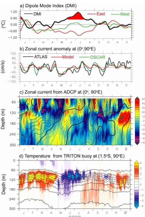
Temporal evolution of DMI together with anomalous subsurface zonal currents and temperature structures observed in the eastern equatorial Indian Ocean during January-December 2008 are presented in Figure 4. The SST anomalies in both eastern and western poles were negative from February and are associated with the basin-wide cooling as described in the previous section. Positive DMI started to develop in late April (Fig. 4a), when the zonal currents indicated westward anomalies (Figs. 4b-c). The DMI rapidly increased in May as the western pole became warmer, and continued to increase and exceeded its one standard deviation (0.48) at the end of May (Fig. 4a).
Fig. 3.SST (shaded) and surface wind (vectors) anomalies averaged for (a) December 2007-February 2008 (DJF), (b) March-May 2008
The eastward flowing Wyrtki jet that occurs during the monsoon transition period in April/May was absent during the spring of 2008 (Figs. 4b-c). The observed near-surface zonal currents indicated anomalous westward currents in May, which were opposite to the climatological conditions. The anomalous westward currents in the thermocline depth were observed from March, two months earlier than that in the upper layer (Fig. 4c). By mid-May, anomalous westward currents were observed from the near surface down to a depth of about 120 m, with a maximum value of about 50 cm/s. The zonal currents remained westward until July though there was relatively weak short-term variability, showing the alternating eastward and westward currents associated with the intra-seasonal atmospheric oscillations during June-July. During the peak phase of the IOD in June-July, strong eastward undercurrents in the layer between about 90 m and 150 m were observed, and this is opposite to normal conditions (Fig. 4c).
There was a subsurface signal for the evolution of the IOD event, as was described in a previous study concerning the 2006 IOD event. Horii et al. (2008) found negative subsurface temperature anomalies in May, three months before the onset of the 2006 IOD event and continued for several months after the termination of the IOD event (see their Fig. 2b). In contrast, in this study we found that the initiation of negative temperature anomalies in the thermocline in late April 2008 (Fig. 4d) co-occurred with the development of the DMI (Fig. 4a). The negative anomaly lasted only about 4 months until August before it gradually changed to a positive anomaly in September. A maximum negative anomaly of about -4°C occurred during the peak phase of the IOD in June-July, during which a spreading of the subsurface isotherm occurred.
A rapid decrease in the DMI in July (Fig. 4a) coincided with strong eastward currents observed from the near surface down to a depth of about 120 m (Figs. 4b-c). The DMI remained constant from the end of July until mid-August before it rapidly decreased and completely disappeared in September (Fig. 4a). Note that the second decrease in the DMI in late-August also coincided with eastward zonal currents (Figs. 4b-c). This may indicate the relative importance of the zonal heat advections during the termination of the 2008 IOD event.
In order to evaluate the role of the zonal heat advections during the termination of the 2008 IOD event, we considered the mixed layer temperature balance, which can be written as
. (1)
The term on the left hand side represents a local storage. Whereas the terms on the right hand side indicate the atmospheric heating by the net surface heat flux across the
air-sea interface (Q0) and the heat loss by shortwave
radiation penetrating below the mixed layer (Qpen), and the
horizontal advection and the residual term, which consists of components that we could not estimate directly from the
h∂T
∂t
--- Q0+Qpen ρCp
---–hv⋅∇T+R =
data, such as the vertical heat fluxes from the bottom of the mixed layer and horizontal and vertical diffusivity. Note that a positive sign is used for the surface flux terms when they represent gains to the mixed layer. Penetrative radiation, Qpen, was calculated based on shortwave radiation and mixed
layer depth as Qpen = -0.47 Qshort exp(-γh), with g = 0.04 m -1
(Wang and McPhaden 1999). In addition, we define h as a
mixed layer depth, ρ as seawater density, and Cp as heat
capacity. T and v are mixed layer temperature and horizontal velocity, respectively.
The net surface het flux (Q0) was estimated as
Q0= (1 -α) Qshort + Qlong + Qlatent+ Qsensible, (2)
where a is the albedo and it is defined to be a constant value of 0.055 (Kumar et al. 2011). Qshort is the incoming shortwave
radiation, Qlong is the net outgoing longwave radiation, Qlatent
is the latent heat flux, and Qsensible is the sensible heat flux.
The combination of Q0 and Qpen represents the net surface
heat flux absorbed by the mixed layer.
The time rate of change of the mixed layer temperature
(∂T/∂t) is estimated using TRMM SST. We computed the
monthly averaged mixed layer depth (h) using temperature
and salinity profiles from Argo floats during 2005-2009.
The mixed layer depth (h) is estimated using a density
criterion, in which h is defined by specifying a density
difference of 0.2 kg m-3 from the surface value (Sprintall and Tomzack 1992).
Following Lee et al. (2004), we estimated the horizontal advection as
, (3)
where u and v represent zonal and meridional velocity averaged at the mixed layer, respectively. Here, we estimated u and v using OSCAR data, which represent the velocity at 15 m
depth. δT is the difference between SST and SST averaged
in the region of interest, and ∆x and ∆y are the distances along the zonal and meridional boundaries of the region, respectively. The subscripts w, e, s, and n represent averages along the western, eastern, southern, and northern boundaries, respectively.
For a quantitative assessment of the contribution of zonal heat advection on the mixed layer temperature balance, we focused on the eastern equatorial Indian Ocean region (80°E - 93°E, 4°S - 2°N). Our selection of this region is based on two factors. First, the region is located on the
equatorial waveguide. Therefore, the role of equatorial waves in generating SSTA in this region can be resolved. Second, based on our quantitative analysis, the SSTA in this region represents the SSTA in the eastern pole of the IOD, where the correlation between two time series is larger than 0.8 with a significant level above 95% (Fig. 5b).
Figures 5c shows the temporal evolution of the local temperature variation, the zonal and meridional heat advection, and the total heat flux during March-September 2008. It is shown that there is cooling tendency of (∂T/∂t during the development of the IOD event in late May. This cooling event was consistent with a negative trend in the zonal heat advection, while it was opposite to the surface heat flux. By early July, the cooling tendency was terminated and then the warming tendency of (∂T/∂t took place in the mid-July just after the peak phase of the IOD event. This warming event was consistent with the positive trend in the zonal heat advection and coincided with the rapid decrease in the DMI time series (Fig. 5a). This suggests the importance of the zonal heat advection during the termination of the IOD event, which provides a favorable condition for the v⋅∇T (uwδTw)+(ueδTe)
∆x
--- (usδTs)+(unδTn) ∆y ---+
=
Fig. 5.(a) Reproduced from Fig. 1a, except for the period of
surface heat flux to warm the SST in the eastern equatorial Indian Ocean.
5. Role of Equatorial Waves
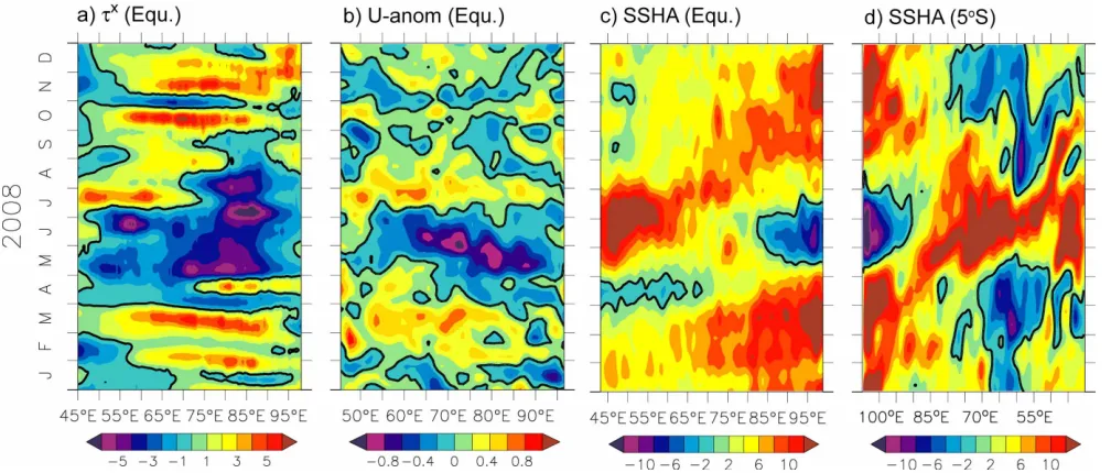
In this section we investigate the basin-scale surface layer variability associated with the 2008 IOD, focusing on the role of equatorial waves. Figure 6 shows time-longitude diagrams of the anomalous zonal wind stress, zonal current and SSH anomalies along the equator together with SSH anomaly along 5°S. During January-March, strong anomalous westerly wind stress along the equator generated strong eastward zonal current and large positive SSH anomalies (downwelling Kelvin waves) along the equator (Figs. 6a-c). At the same time, there were SSH anomalies of the opposite sign (upwelling
Rossby waves) centered along ~5°S in the western basin
(70°E - 40°E), consistent with the sign of the equatorial wind stress anomalies and the equatorial wave theory (Fig. 6d). In addition, the eastern boundary reflection of the downwelling Kelvin wave (positive SSH anomaly) into the westward propagating downwelling Rossby wave was also observed during this period (Fig. 6d).
During the boreal spring of May to early July 2008, the transition period of two monsoons, strong easterly wind anomalies were observed along the equator (Fig. 6a). As a result, the spring Wyrtki jet was reversed completely during this time and a maximum westward zonal current of about 1
m/s was observed in the central basin (Fig. 6b). Meanwhile, a dipole pattern in the SSH anomaly was revealed along the equator indicating a typical positive IOD pattern: the SSH rose more than 15 cm in the western basin while it dropped as much as 10 cm in the eastern basin (Fig. 6b). As the positive IOD was underway, strong equatorial easterly winds promoted the generation of downwelling off-equatorial Rossby waves. This led to the generation of large positive SSH anomalies in the central basin that propagated westward and reached the western boundary in July and reflected back as downwelling equatorial Kelvin waves (Fig. 6d).
Starting from mid July 2008, the equatorial easterly anomalies weakened and were replaced by westerly wind in the western half of the basin (Fig. 6a). These winds forced eastward zonal currents (Fig. 6b) and downwelling Kelvin waves (positive SSH anomaly) and upwelling Rossby waves (negative SSH anomaly) in the equatorial waveguide (Figs. 6c-d). In August, relatively weaker westerly winds were observed in the central and eastern basin (Fig. 6a) that generated a weak eastward zonal current (Fig. 6b) and enhanced the positive (negative) SSH anomalies in the equatorial waveguide (Figs. 6c-d). At that time the dipole pattern in SSH anomaly had completely disappeared.
In order to examine quantitatively the role of wind-forced and reflected equatorial waves in the evolution of the 2008 IOD, we evaluated the results of our linear wave model. The model affords an opportunity to diagnose the wave
Fig. 6.Time-longitude diagrams of (a) zonal wind stress anomaly (×10-2 N/m2), (b) zonal current anomaly (m/s), (c) SSH anomaly
processes involved in the evolution of the 2008 IOD event as its output can easily be separated into wind-forced and boundary-reflected waves. Here, we evaluated separately the relative importance of wind-forced and boundary-reflected waves in generating zonal currents during the evolution of 2008 IOD event.
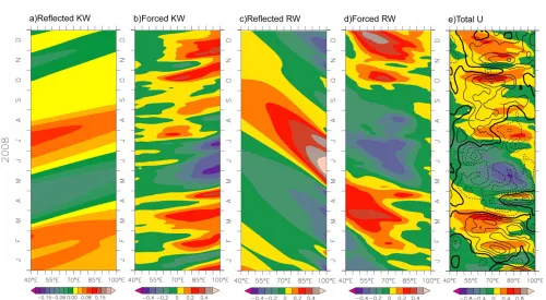
Figure 7 shows the evolution of the zonal current anomalies induced by the wind-forced and boundary-generated waves during 2008. Prior to the IOD, intense intra-seasonal eastward zonal currents appeared during January-April 2008 (Fig. 7e). Apparently, these eastward zonal currents were mainly due to wind-forced waves (Fig. 7b,d). In the western basin, the zonal current variations were mostly influenced by the wind-forced Rossby waves (Fig. 7d). On the other hand, the wind-forced Kelvin and Rossby waves have a comparable contribution on the zonal current variations east of about 70°E.
During May-June, there were strong westward zonal currents with the maximum amplitude located in the about
70°E - 90°E associated with basin-wind easterly wind
anomalies (Fig. 7e). The zonal currents generated by the wind-forced Kelvin and Rossby waves were also westward
during this period, and the locations of their maxima correspond well to that of the total solution (Figs. 7b, d). The reflected Rossby waves were eastward from May until August and have maximum amplitude at the eastern boundary (Fig. 7c). One can see the contribution of reflected Rossby waves on the total zonal current anomalies is eastward anomalies near the eastern boundary during the peak phase of the IOD event in May-June though the wind anomalies continue to be westward (Fig. 7e). In addition, the westward progression of the zonal current anomalies during this period was associated with the wind-forced Rossby waves as previously suggested (Nagura and McPhaden 2010b). Note that the contributions from the western-boundary-generated Kelvin waves were much smaller than those from wind-forced waves (Figs. 7a,c).
During the termination period of the IOD in mid-July, a strong eastward zonal current was detected, with its maximum located around 80°E - 95°E (Fig. 7e). During this period, the easterly wind anomalies in the eastern basin weakened, while in the western basin they changed into westerly ones (Fig. 7e). The later forced eastward zonal currents associated with downwelling Kelvin waves with maximum amplitude
Fig. 7.Time-longitude diagrams of model zonal current anomalies at 15 m depth along the equator for January-December 2008, from (a)
located around 55°E - 75°E (Fig. 7b). At the same time, the eastern-boundary-reflected Rossby waves associated with the wind-forced Kelvin waves in early July, generated strong eastward zonal currents that propagated westward with a maximum amplitude located near the eastern boundary (Fig. 7c), close to the maximum in the total solution (Fig. 7e). The decomposition of wind-forced and boundary-generated waves indicates that the eastward zonal currents during this period were mostly due to the eastern-boundary-reflected Rossby waves (Figs. 7c,e).
Eastward zonal currents appeared again in late-August/
early-September with maximum amplitude around 70°E
-90°E (Fig. 7e). These eastward currents were associated
with a strengthening (weakening) of westerly winds in the central (eastern) basin (Fig. 7e). The decomposition of wind-forced and boundary-generated waves indicates that the eastward zonal currents during this period were mostly due to the wind-forced Kelvin waves (Fig. 7b,e).
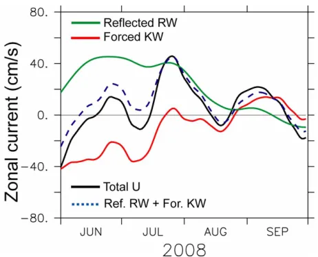
In order to explicitly assess the causes of the eastward zonal current variability observed in the eastern equatorial Indian Ocean during the termination of IOD, we plot each component of the wind-forced and boundary-generated equatorial waves averaged over the region of 80°E - 93°E, 4°S - 2°N (Fig. 8). Apparently, it is shown that the eastward zonal current appeared in mid-July was strongly influenced by the eastern-boundary-reflected upwelling Rossby waves, although the contribution from the wind-forced downwelling
Kelvin waves was not negligible. This result is in agreement with our observation result shown in the previous chapter. Note that the contributions from the wind-forced Rossby and the reflected Kelvin waves were negligible (not shown)
6. Discussion and Summary
In this study, we examine the role of equatorial waves during the evolution of the 2008 IOD event using available observational data and output from a continuously stratified long wave model. The present observational results indicate that three consecutive positive IOD events took place in the tropical Indian Ocean through 2006-2008 (Cai et al. 2009). The 2006 positive IOD was a strong event that was followed by a weak El Niño event in the Pacific (Fig. 1). Uniquely among recent occurrences of the IOD events, the 2006 positive IOD event was followed by another positive event in 2007 though with a relatively weaker amplitude (Fig. 1a). The return of positive IOD in 2007 is particularly surprising since the generally accepted paradigm for the IOD assumed a quasi-biennial periodicity in IOD variability (Saji et al. 1999). Interestingly, the 2007 positive IOD event occurred while the Pacific Ocean showed an evolution of a La Niña event (Fig. 1b). In a typical La Niña event, two Walker cells with ascending branch over the Maritime Continent took place in the Indian and Pacific oceans. This atmospheric circulation is unfavorable for the development of the positive IOD event. However, during 2007 there were, unusually, three Walker cells with two ascending branches over the warm SST anomalies in the western Indian Ocean and in the western Pacific (Behera et al. 2008). This led to the presence of easterly anomalies during boreal spring that triggered the positive IOD event in 2007.
A positive IOD event returned in boreal summer 2008 when the Pacific Ocean displayed normal conditions (Fig. 1). The 2008 positive IOD event was an early matured and abruptly terminated event: developed in April, matured in July, and diminished in September (Fig. 3). The evolution of the 2008 IOD is linked to the equatorial wave dynamics. Our observations have shown that during the peak phase of the event in May-June, the easterly wind anomalies generated upwelling equatorial Kelvin waves (negative SSH anomaly) and downwelling off-equatorial Rossby waves (positive SSH anomaly) (Figs. 6a,c-d). In addition, the spring Wyrtki jet was reversed completely during this period with maximum amplitude of about 1 m/s observed in the central basin (Fig. Fig. 8.Time series of zonal current anomaly at 15-m depth averaged
6b). Moreover, the observation also revealed a clear westward progression of the surface zonal currents during the peak phase of the event. During the termination of the IOD in mid-July 2008, easterly wind anomalies in the eastern basin were weakened and were replaced by westerly wind anomalies in the western half of the basin. At the same time, we observed strong eastward zonal currents and positive SSH anomaly along the equator suggesting the important role of the equatorial waves in the termination of the event.
We then evaluated the relative roles of the wind-forced and boundary-generated waves in the evolution of the 2008 IOD event using a simple linear wave model. The model shows that the wind-forced Rossby waves dominated the zonal current variations near the western equatorial Indian Ocean prior to the IOD (Fig. 7d), whereas in the central and eastern equatorial region the wind-forced Kelvin and Rossby waves have a comparable contribution (Figs. 7a, 7d). Similarly, the zonal current variations during the peak phase of the IOD in May-July are mostly influenced by the forced Rossby waves, though contributions from the wind-forced Kelvin waves in the central basin were not negligible. It is interesting to note that the zonal currents near the eastern boundary were eastward just after the onset of the IOD though the wind anomalies continued to be westward (Fig. 7e). These eastward anomalies were due to the eastern-boundary-generated Rossby waves (Fig. 7c). The dominant contribution of the Rossby waves to the zonal current variations can be seen on the westward progression of the anomalies prior to and during the peak phase of the IOD. Cai et al. (2009) highlighted the importance of off-equatorial upwelling Rossby waves in generating the 2008 IOD event. They suggested that those upwelling Rossby waves were reflected back into the interior Indian Ocean as a series of upwelling equatorial Kelvin waves after reaching the western boundary. Note that the off-equatorial upwelling Rossby waves were generated by westerly wind anomalies along the equator. Thus, the work by Cai et al. (2009) has shown the important role of off-equatorial Rossby waves in the development of the 2008 IOD event.
On the other hand, in this study we highlighted the role of eastern-boundary-reflected Rossby waves in the abrupt termination of the 2008 IOD event. It was shown that the termination of the 2008 IOD in mid-July was co-occurring with the presence of eastward zonal currents along the equator (Fig. 7e). We found that these eastward zonal currents were mostly due to the eastern-boundary-reflected upwelling
Rossby waves, although the contribution from the wind-forced downwelling Kelvin waves was not negligible (Fig. 8). This eastward zonal current terminated the negative zonal heat advection and co-occurred with the warming tendency in the eastern equatorial Indian Ocean (Fig. 5b). This suggests that the zonal heat advection induced by the eastward zonal currents during the termination of the 2008 IOD event plays important role in providing a favorable condition for the surface heat flux to warm the SST in the eastern basin. In addition, our results also show that the role of western-boundary-reflected upwelling Kelvin waves was negligible during the development of the 2008 IOD event (Fig. 7a).
Acknowledgments
The work was supported by the Indonesia Toray Science Foundation (ITSF) through the Science and Technology Research Grant 2012, and by the University of Sriwijaya through Penelitian Unggulan Perguruan Tinggi 2012. The author gratefully acknowledges the helpful discussions with and suggestions from Michael J. McPhaden. The author also thanks Motoki Nagura for the model output. This is CGCCS contribution 1302.
References
Behera SK, Luo J-J, Yamagata T (2008) Unusual IOD event of 2007. Geophys Res Lett 35:L14S11. doi:10.1029/2008GL034122 Bonjean F, Lagerloef GSE (2002) Diagnostic model and analysis of the surface currents in the tropical Pacific Ocean. J Phys Oceanogr 32:2938-2954
Cai W, Pan A, Roemmich D, Cowan T, Guo X (2009) Argo profiles a rare occurrence of three consecutive positive Indian Ocean Dipole events, 2006-2008. Geophys Res Lett 36:L08701. doi: 10.1029/2008GL037038
Chambers DP, Tapley BD, Stewart RH (1999) Amomalous warming in the Indian Ocean coincident with El Niño. J Geophys Res 104:3035-3047. doi:10.1029/1998JC900085
Clarke AJ, Liu X (1993) Observations and dynamics of semiannual and annual sea level near the eastern equatorial Indian Ocean boundary. J Phys Oceanogr 23:386-399
Feng M, Meyers G (2003) Interannual variability in the tropical Indian Ocean: a two-year time-scale of Indian Ocean Dipole. Deep-Sea Res 50:2263-2284
Fu LL (2007) Intraseasonal variability of the equatorial Indian Ocean observed from sea surface height, wind, and temperature data. J Phys Oceanogr 37:188-202
Lett 35:L03607. doi:10.1029/2007GL032464
Iskandar I, Masumoto Y, Mizuno K (2009) Subsurface equatorial zonal current in the eastern Indian Ocean. J Geophys Res 114:C06005. doi:10.1029/2008JC005188
Kumar BP, Vialard J, Lengaigne M, Murty VSN, McPhaden MJ (2011) TropFlux: air-sea fluxes for the global tropical oceans-description and evaluation against observations. Clim Dynam 38(7-8):1521-1543. doi:10.1007/s00382-011-1115-0 Lau NC, Nath MJ (2003) Atmosphere-Ocean Variations in the
Indo-Pacific Sector during ENSO Episodes. J Climate 16:3-20 Le Blanc J-L, Boulanger J-P (2001) Propagation and reflection of
long equatorial waves in the Indian Ocean from TOPEX/ POSEIDON data during 1993-1998 period. Clim Dynam 17:547-557. doi: 10.1007/s003820000128
Lee T, Fukumori I, Tang B (2004) Temperature advection: internal versus external processes. J Phys Oceanogr 34:1936-1944 McPhaden MJ, Meyers G, Ando K, Masumoto Y, Murty VSN,
Ravichandran M, Syamsuddin F, Vialard J, Yu L, Yu W (2009) RAMA: The Research Moored Array for African-Asian-Australian monsoon analysis and prediction. Bull Am Meteorol Soc 90:459-480
Meyers GA, McIntosh PC, Pigot L, Pook MJ (2007) The year of El Niño, La Niña, and interactions with the tropical Indian Ocean. J Climate20:2872-2880
Moore DW, Philander SGH (1977) Modelling of the tropical oceanic circulation. In: Goldberg ED, McCave IN, O’Brien JJ, Steele JH (eds) The Sea, vol. 6. John Wiley and Sons, pp 319-361
Murtugudde R, McCreary JP, Busalacchi AJ (2000) Oceanic processes associated with anomalous events in the Indian Ocean with relevance to 1997-1998. J Geophys Res 105 (C2):3295-3306
Nagura M, Mcphaden MJ (2010a) Wyrtki jet dynamics: Seasonal variability. J Geophys Res 115:C07009. doi:10.1029/2009JC005922 Nagura M, Mcphaden MJ (2010b) The dynamics of zonal current
variations associated with the Indian Ocean Dipole. J Geophys Res 115:C11026. doi:10.1029/2010JC006423
Rao SA, Behera SK, Masumoto Y, Yamagata T (2002) Interannual
subsurface variability in the tropical Indian Ocean with a special emphasis on the Indian Ocean dipole. Deep-Sea Res 49:1549-1572
Rao SA, Yamagata T (2004) Abrupt termination of Indian Ocean dipole events in response to instraseasonal oscillations. Geophys Res Lett 31:L19306. doi:10.1029/2004GL020842
Rao SA, Luo J-J, Behera SK, Yamagata T (2009) Generation and termination of Indian Ocean dipole events in 2003, 2006 and 2007. Clim Dynam 33:751-767. doi:10.1007/s00382-008-0498-z Reppin J, Schott FA, Fischer J, Quadfasel D (1999) Equatorial
currents and transports in the upper central Indian Ocean: annual cycle and interannual variability. J Geophys Res 104 :15495-15514. doi:10.1029/1999JC900093
Saji NH, Goswami BN, Vinayachandran PN, Yamagata T (1999) A dipole mode in the tropical Indian Ocean. Nature 410 :360-363
Vinayachandran PN, Saji NH, Yamagata T (1999) Response of the equatorial Indian Ocean to an unusual wind event during 1994. Geophys Res Lett 26:1613-1616. doi:10.1029/1999GL900179 Vinayachandran PN, Kurian J, Neema CP (2007) Indian Ocean
response to anomalous conditions in 2006. Geophys Res Lett 34:L15602. doi:10.1029/2007GL030194
Webster PJ, Moore AW, Loschnigg JP, Leben RR (1999) Coupled ocean-atmosphere dynamics in the Indian Ocean during 1997-1998. Nature 401:356-360
Weisberg RH, Wang C (1997) Slow variability in the equatorial west-central Pacific in relation to ENSO. J Climate 10 :1998-2017.
Wyrtki K (1973) An equatorial jet in the Indian Ocean. Science 181:262-264
Yamagata T, Behera SK, Luo J-J, Masson S, Jury M, Rao SA (2004) Copled ocean-atmosphere variability in the tropical Indian Ocean. Earth Climate: The Ocean-Atmosphere Interaction. AGU, Geophys Monogr No. 147, pp 189-212