Estimating willingness to pay by risk
adjustment mechanism
Joo Heon Parka,* and Douglas L. MacLachlanb
aDepartment of Economics, Dongduk Women’s University,
23-1 Wolgok-dong, Sungbuk-Gu, Seoul 136-714, Korea
bMichael G. Foster School of Business, University of Washington, Seattle,
WA 98195-3226, USA
Measuring consumers’ Willingness To Pay (WTP) without considering the level of uncertainty in valuation and the consequent risk premiums will result in estimates that are biased toward lower values. This research proposes a model and method for correctly assessing WTP in cases involving valuation uncertainty. The new method, called Risk Adjustment Mechanism (RAM), is presented theoretically and demonstrated empiri-cally. It is shown that the RAM outperforms the traditional method for assessing WTP, especially in a context of a nonmarket good such as a totally new product.
Keywords: purchase decisions; willingness to pay; contigent valuation
method; adjustment mechanism
JEL Classification: D12; D81; M31
I. Introduction
Traditional consumer theory presumes that a con-sumer makes a purchasing decision by comparing his or her own subjective value of a good (or service) with its objective value. The objective value is the posted price, while the subjective value is usually measured by the so-called Willingness To Pay (WTP) that is defined as the maximum dollar amount a consumer is willing to pay for the good. If the posted price is below a consumer’s WTP, the purchase would be made; otherwise the purchase would be abandoned. We call this the Traditional Decision Mechanism (TDM).
A problem from the researcher’s perspective is that a consumer never reveals his or her own WTP directly, so that the WTP is not observable, whereas
the price is directly observed in a market.
However, consumers reveal their WTP indirectly
through transactions, so that their WTP can be estimated by analysing their observed transaction behaviours. While the TDM provides a theoretical basis for inferring the WTP from purchase behav-iours, it makes sense only when there is no uncer-tainty in consumers valuing the good of interest. If consumers are uncertain over the value they place on the good and do not know their WTP exactly as a single value, they are unable to compare their WTP with the price. Therefore, the TDM should not be employed as a basis for inferring WTP for a good when uncertainties are involved in valuation of the good.
A question for us is how consumers make decisions to purchase a good or not if they are ignorant of their WTP for the good as a single value because of uncertainties. As an answer, we propose a new
purchasing decision mechanism called a Risk
Adjustment Mechanism (RAM) that can be applied
*Corresponding author. E-mail: [email protected]
Applied EconomicsISSN 0003–6846 print/ISSN 1466–4283 online!2013 Taylor & Francis 37 http://www.informaworld.com
under valuation uncertainty. A key characteristic of RAM is that consumers are presumed to have in their minds a statistical distribution of their WTP instead of a single value. Furthermore, typically risk averting consumers are expected to purchase a good if the mean of their WTP is greater than the good’s price by at least their risk premium. This is in contrast to TDM in which consumers are expected to purchase a good if their WTP is simply greater than the price. If consumers are assumed to have aversion to risk, the WTP of consumers using RAM who have decided to purchase must be sufficiently greater than the price, while it is theoretically enough to purchase for consumers using TDM that the WTP be just greater than the price even by a single penny. Therefore, from a RAM point of view, the empirically assessed TDM underestimates WTP by structure, since the TDM devalues the WTP of a risk averting consumer at least by his or her positive risk premium.
The notion that consumers are uncertain about valuation is not new. Uncertainty in valuation has been addressed by many researchers in a number of
different ways since Ready et al. (1995) raised the
issue explicitly in a context of Contingent Valuation Method (CVM).
In fact, there are many well-known uncertain factors that can and do influence a consumer’s valuation. Wang (1997) argued that uncertainty
might exist in a commodity or service itself,1 in an
unpredictable market situation, in socio-demographic variables, and in people’s uncertain preferences, among others. Recognizing the existence of such uncertainties, various studies have been made that incorporate the uncertainties into the valuation process.
Van Kootenet al. (2001) employed fuzzy set theory
to represent the underlying vagueness of preferences. Hanemann and Kristro¨m (1995) and Wang (1997) suggested adding a random variable to the utility function. But they do not take the consumer’s behaviour into account, in contrast with our pro-posed RAM where the risk premium reflecting the consumer’s behaviour against uncertainties plays an explicit role in the purchasing decision.
Consumers react to uncertainties in different ways, leading to different market results. Mauro and Maffioletti (2004) recognized consumers’ reaction to uncertainties in the face of an incentive compatible
mechanism through experiments, and suggested that ambiguity may be a relevant factor that affects market prices and allocations. And a purchasing decision mechanism like RAM that reflects con-sumers’ means of dealing with uncertainties can also explain more efficiently the market results of a new product with embedded uncertainties. For example, we may also explain through the RAM the behaviour difference between early adopters and slow movers for new products.
Studies on how uncertainties affect the purchasing decisions have been usually made in a hypothetical context such as the CVM because the consumers’ attempts to resolve uncertainties are not observed directly in real markets. We cannot deduce the consumers’ uncertainty resolution behaviours from their purchasing decisions.
However, valuation based on a CVM is often questioned because of the so-called hypothetical bias caused by difference in respondents’ behaviour between a hypothetical situation and a real purchase
situation (Paradiso and Trisorio, 2001). Champet al.
(1997), Johannessonet al. (1998) and Alberiniet al.
(2003) used a calibration process with follow-up questions regarding the certainty of the stated valu-ation in a CVM context in order to reduce the hypothetical bias; for example, ‘very uncertain’, ‘not likely’, ‘very sure’ and so on. But these assessments of certainty could be as wrong as the valuation reports because the assessments are also asked in the same hypothetical situation as the valuation. Contrary to these approaches, the RAM does not have the bias problems caused by double sources of uncertainty because it incorporates uncertainties into the model instead of trying to handle uncertainties outside the model. And furthermore, the RAM can explain and reduce the hypothetical bias because it contains a risk premium variable that should be measured in the same situation where a product is evaluated.
Arielyet al. (2003) and Hanleyet al. (2009) posited
that consumers probably have some range of accept-able values rather than specific WTP value for a good. Following their thinking, we might assume that consumers have in their heads a distribution of WTP values rather than a single value. This assumption has been used explicitly or implicitly by many researchers
such as Cameron and Quiggin (1994),2Carson et al.
(1994) and Wang (1997).
1One would face uncertainty over how much gains could be obtained from a nonmarket good that has never before existed.
Such uncertainty would not be removed until the good is actually consumed. For example, the value of improved environment is not realized until it is actually provided and consumed.
2Cameron and Quiggin (1994) said ‘Respondents seem not to hold in their heads a single immutable ‘true’ point valuation
....
Wang (1997) and Changet al. (2007) among others asked a polychotomous choice WTP question with an implicit assumption that the certainty of a respon-dent’s answer depends upon the difference between the WTP distribution and the bid price. Especially, Wang (1997) allows the trichotomous response options of ‘yes’, ‘no’ or ‘don’t know (DK)’. In his model, there is a vagueness band over which a respondent has an option of ‘DK’ instead of making a clear purchasing decision. It should be noted that ‘DK’ option is never allowed by structure in a real purchase situation. The true outcomes made by individuals in a real situation are only either ‘yes’ or ‘no’. The RAM has only dichotomous options of ‘yes’ or ‘no’, which is consistent with real market transactions.
In the next section, the RAM is formally intro-duced along with the TDM. In Section III, the estimation issue is addressed. An empirical compar-ison of WTP estimates by TDM and RAM is made in Section IV to see how seriously the TDM underes-timates the WTP. Some concluding remarks follow in the last section.
II. Risk Adjustment Mechanism
A consumer decides to purchase a good (z) if his
or her utility can be increased by purchasing the good, i.e.
whereU(.) is an indirect utility function; yi denotes
theith consumer’s income;pis the price vector of all
other goods except good z;p(z) the price of goodz;
wi&(z) theith consumer’s WTP for the goodzandIiis
a binary response variable taking one for purchasing
and zero for not purchasing goodz.
Since the WTP for a good is the maximum amount of money that a consumer is willing to give up in exchange for the good without decreasing the initial utility level, the utility change caused by purchasing a good is exactly the same as that caused by changing the consumer’s income by the difference between the price and the WTP for the good. Therefore the left-hand side of the inequality in Equation 1 is the
utility level after purchase that theith consumer could
attain by purchasing goodz with its pricep(z) paid
while the right-hand side is the utility level before purchase. To sum up, a consumer purchases a good if
the utility after purchase is greater than the utility before purchase.
Since the indirect utility function is monotonically
increasing in income y, the purchasing decision
mechanism (Equation 1) may be converted simply as follows:
Ii¼1 ifw&iðzÞ 'pðzÞ
Ii¼0 otherwise
ð2Þ
The mechanism (2) means that a consumer pur-chases a good if the WTP is greater than the price, which is usually presumed the purchasing mechanism by traditional consumer theory and is called the TDM in this article.
It is worth noting that the TDM works correctly only if there is no uncertainty related with the purchase. The TDM can be applied only when a consumer knows his or her own WTP exactly as a single value with certainty, and then can compare the WTP with the price as suggested by Equation 2. However, the decision mechanism is not as simple as in Equation 2 if uncertainties are involved. Suppose uncertainties stem from the benefits expected from consuming a good z, the WTP is also uncertain and should be treated as random because it totally depends upon the benefits. Since the benefits of a good are actually realized by consuming the good, a consumer cannot know his or her WTP for the good precisely until he or she consumes it. Therefore, a consumer can only guess the WTP at the purchase time when actual consumption is not yet realized. In this article, the WTP realized after consumption is
called theex postWTP and the WTP guessed before
consumption is called theex anteWTP.
There is usually a difference between the ex post
andex ante WTP’s, which depends upon the degree
of uncertainty. Hanleyet al. (2009) argued that this
kind of uncertainty is reduced when a person has more experience, i.e. the uncertainty might be inversely related with experience with the good. One would expect little difference between the two WTP’s for standard and frequently used goods, because consumers have already considerable experiences with the amount of benefit that they can expect from those goods. Contrarily, one would expect a
large difference betweenex post andex anteWTP’s
for the goods such as totally new products or nonmarket goods that have never been traded in a market before. Consumers are ignorant of how much benefit they can obtain from such goods until actual
consumption.3
3Although the
ex postWTP is a more accurate indicator of the true value of a good and it would be desirable to know that
value when doing a cost benefit analysis and developing public policy, only theex anteWTP is typically known or knowable
At the purchase time, theex postWTP is random
and is assumed to be distributed around theex ante
WTP as
wiðzÞ ¼w&iðzÞ þui, E u½ ) ¼i 0, Var½ ) ¼ui !u2 ð3Þ
where ui is an error term reflecting uncertainties
associated with consumption;wi(z) theex postWTP;
wi&(z) theex anteWTP. Note that the consumers are
posited to guess their ownex anteWTP as the mean
value of theex postWTP distribution even at the time
of purchase. And the consumer is exposed to uncer-tainty to a degree of the variance of the error
term (!2
u).
Now consider how a consumer would make a purchasing decision when facing uncertainty and
being ignorant of the ex post WTP. The consumer
should make a purchase if the expected utility is greater than the utility without purchase but other-wise he or she should not. This can be expressed as
Ii¼1 ifEwiðzÞ½U pð ,yi"pðzÞ þwiðzÞÞ) 'U pð ,yiÞ
Ii¼0 otherwise ð4Þ
A consumer tends to avoid uncertainties if possible. A consumer is willing to pay an incremental amount of money if he or she is guaranteed to have a certain offer instead of an uncertain offer. The amount of money a consumer is willing to pay for a certain offer of ensuring the mean value of an uncertain offer instead of the uncertain offer is called the risk premium of the uncertain offer. And the risk
premium of a new good z can be defined as Ri(z)
satisfying the following equation:
U p,yi"pðzÞ þw&iðzÞ "RiðzÞ
! "
¼EwiðzÞ½U pð ,yi"pðzÞ þwiðzÞÞ) ð5Þ Therefore, combining Equations 5 and 4 and using
the fact that the indirect utility function U(.) is a
monotonically increasing function, yields the follow-ing purchasfollow-ing decision mechanism:
Ii¼1 ifw&iðzÞ "pðzÞ 'RiðzÞ
Ii¼0 otherwise
ð6Þ
which we call the RAM. A consumer purchases the
goodzif his or herex anteWTP exceeds the price at
least by the risk premium; the consumer should not purchase otherwise. This is a salient point differen-tiating the RAM from the TDM. Note that if there is no uncertainty and the risk premium is zero, then the RAM coincides with the TDM exactly. Actually,
the TDM need not distinguish the ex ante WTP
from theex postWTP since it assumes no uncertainty
at all. If the WTP is greater than the price even by a miniscule value, the purchase should be made
theoretically by TDM, but the purchase should not be always made by RAM. The RAM considers consumers who decide to purchase the good as having a much higher WTP than the price while the TDM regards them as having just higher WTP than the price. And thus the TDM would yield an
underestimation of WTP when there are
uncertainties.
III. Estimation
The RAM presented as in Equation 6 implies that
consumers take their ownex anteWTP together with
the price and risk premium into account to make a
purchase decision. Theex anteWTP is assumed to be
linearly determined as
w&
iðzÞ ¼x
0
i"þ"i, "i*Nð0,!"2Þ ð7Þ
where xi is a vector of covariates, " the vector of
coefficients and"ithe error term. Now the error terms
in Equation 7 should be distinguished from those in Equation 3. The error term in Equation 3 denotes a
part ofex postWTP that a consumer cannot grasp at
the purchasing stage and is the source of uncertainty.
But the error term"iin Equation 7 denotes a part of
the ex ante WTP that a researcher cannot explain with a vector of covariates even though a consumer knows it completely. So the researcher regards the ex ante WTP as being statistically distributed even though a consumer knows it as a single value.
The log-likelihood functions implied by TDM and RAM are presented as in Equations 8 and 9, respectively.
where!S(+) is the cumulative distribution function of
the standardized normal distribution.
the inequality condition of TDM can be converted as
can be identified only up to a scale transformation because
#0þ"1xi1þ + + + þ"1kxikþ"i'0
,$ð#0þ"1xi1þ + + + þ"1kxikþ"iÞ '0 for$40
ð11Þ
The TDM cannot predict the value of WTP, but only the probability of the inequality condition of TDM being satisfied.
In contrast, the RAM can identify all coefficients fully because different risk premiums are taken by each consumer, even when a common price is given to them. The inequality condition of RAM being multiplied by a positive number, all coefficients can be identified because the multiplication number ($) can be estimated as the coefficient of the risk
premium (Ri(z)) as
However, the above identification of RAM is possible only when the risk premium is observable. Yet in reality this does not occur. The risk premium
associated with the good zis not actually observed.
We need to assume a model of risk premium and then estimate it. It is already proven that there exists a particular relationship like Equation 13 between the risk premium and the attitude toward the risk if the expected return of a risky offer is relatively very small (Malinvaud, 1985).
whereRiis the risk premium for a risky offer with its
variance !2, and ri the Arrow–Pratt absolute Risk
Aversion Index (ARAI) reflecting a person’s attitude toward risk. A respondent with a higher ARAI has a higher risk premium. Now if a Constant Absolute
Risk Aversion (CARA) utility function (Equation 14)
is assumed for simplicity, then the ARAI is fixed atri
whatever the consumer’s income (y) level is
CARA utility function:UðyÞ ¼ "1
ri
e"riy ð14Þ
Assuming that each consumer has a CARA utility function, the log-likelihood of RAM (Equation 9) can be transformed as
the RAM turns out not to be identifiable because a
parameter !2u is added. So we need an additional
assumption to make the model parameters identified. For simplicity, we assume that the degree of uncer-tainty a researcher faces is exactly the same as that
amount a consumer faces, i.e. !u2¼!2". Then the
log-likelihood of Equation 15 becomes identifiable
because the new parameter!2
uis out of the estimation
process.
The log-likelihood functions of Equation 15 are, however, based upon market transactions so that they cannot be applied to the estimation of WTP for a nonmarket good such as a totally new product. By definition no transaction of a nonmarket good has been made and no information pertaining to the market such as the price is available to be observed. Hence a different method is needed to estimate the WTP for a nonmarket product.
The CVM has been used extensively for estimating the value of nonmarket goods. See for example,
Cummings et al. (1986) and Carson and Mitchell
(1994).4The CVM has also been employed as a
pre-test-market evaluation method in the marketing arena (Cameron and James, 1987; Wertenbroch and Skiera, 2002).
The CVM uses a sample survey asking respondents to value a nonmarket good of interest in a hypothet-ical situation where no actual transaction is required. And we are free to give each respondent different prices in CVM because the respondents are supposed to answer ‘yes, I’ll buy it’ or ‘no, I won’t buy it’ with the price given to them. Then the log-likelihood
functions of TDM and RAM with CARA
4
assumption are somewhat changed as follows:
It should be noted that there is no parameter identification concern for both TDM and RAM in
Equations 16 and 17 because!"can be identified as
the inverse of the coefficient of pi(z). All the
coeffi-cients are fully identified for both TDM and RAM
even without the assumption of!2
u¼!"2.
The last problem that must be solved to make the log-likelihood function workable is that an individual
consumer’s ARAI (ri) cannot be observed directly.
But if we make the assumption of CARA utility, we can infer the ARAI indirectly by observing how the consumer behaves when he or she faces uncertainty and can avoid it by paying some risk premium. If we can observe how much uncertainty is involved and how much risk premium the consumer pays, then we can infer the consumer’s ARAI indirectly by the relationship (13) under the CARA assumption. Once an inferred ARAI is available, maximization of the log-likelihood of RAM (Equation 17) yields the estimates of all parameters in RAM.
Now it should be noted that the reason for assuming CARA utility function is that the risk premium in Equation 9 cannot be observed directly. With CARA utility function, we can present the risk premium as a (reduced ) function of the ARAI that can be subsequently inferred from observation of another risk averting behaviour. However, the CARA assumption is not necessary to connect the risk premium with the ARAI. Actually, the risk premium is a function of the ARAI with any utility function. But we need the CARA utility function in order to get a reduced form like Equation 13 with which the risk premium is substituted so that an estimable likelihood function such as Equation 17 could be obtained. Therefore, if we can observe the
risk premium involved in the purchasing decision, we do not need the CARA assumption but just employ the likelihood including the risk premium itself; otherwise, we should make an assumption like CARA in order to get an estimable likelihood function.
IV. An Empirical Study
In this section, the RAM is compared to TDM with a real CVM data. The CVM data were collected to obtain information about consumers’ WTP for a new customized cell phone service. In this case, a Korean mobile telecommunication company attempts to determine the best rate program for each customer by analysing actual data. The company calculates due amounts for the past 3 months under all rate programmes available to find the lowest due amount and its associated rate programme and then informs customers of this information. This is a totally new service that has never been offered before. Customers are thereby not sure how much benefit they can actually obtain from the service.
Each respondent was asked his or her WTP for the new service in different formats – open-ended or
close-ended.5However, the data set used here is only
the close-ended format data set because both TDM and RAM are designed to be applicable only to a dichotomized reaction of such as ‘yes’ or ‘no’ in the close-ended format. For the close-ended format survey, potential respondents were divided into eight groups to which a bid price was chosen and assigned from eight different predetermined bid prices that are distributed from 2000 Won to 9000 Won.
The survey was fielded around Seoul and its suburbs in South Korea by six trained interviewers for 2 weeks during spring of 2008. We conducted 400 interviews with the close-ended CV formats. Of them, we succeeded in getting 347 responses, resulting in a response rate of 86.8%. Deleting questionnaires for which there were no responses to key questions, we obtained 249 final responses ready to be used in estimation. Table 1 presents the percentages of ‘yes’ votes for each bid price. The higher percentage of ‘yes’ votes occurs with the lower bid prices, which is consistent with the law of demand.
This CV survey is different from others in that, along with the question regarding the WTP for the new product, a respondent was also asked his or her
5
WTP for a gamble from which the ARAI of each respondent could be conjectured. Each respondent was asked to play a gamble in which tossing a coin, a player is paid 15 000 Won if the head is upside, or 5000 Won otherwise. The expected value of the gamble is 10 000 Won. The respondent is asked how much he or she was willing to pay for playing the gamble, in an auction manner. A respondent was asked initially whether he or she were willing to pay 6000 Won or not for the gamble. If the answer was ‘no’ for the initial question, the auction stopped and the WTP for the game was regarded as 5000 Won that was the guaranteed minimum amount to pay back to the player. However, if the answer was ‘yes’, the auction continued by asking the same question but the price raised by 1000 Won, i.e. whether they were willing to pay 7000 Won or not for the game. Subsequently, if the answer was ‘no’, the WTP was regarded as 6000 Won. This process was continued until the respondent gave an answer of ‘no’. But the maximum price given to the respondents was set at 10 000 Won because a risk averting respondent is believed to be willing to pay no more than the expected value of the game.
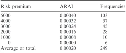
The risk premium of each respondent can be obtained by subtracting the expected return of the game, 10 000 Won from the WTP of each respondent inferred through the series of question items. For example, if a respondent’s inferred WTP for the game is 7000 Won, then his or her risk premium of the game is calculated to be 3000 Won. Then with the CARA assumption, the ARAI can be also calculated by using the relationship (13). Since the variance of the returns of the game is 25 million Won, the ARAI of each respondent is calculated as
ri¼
2RiðgÞ
25 000 000 ð18Þ
where Ri(g) is the risk premium of ith respondent.
The risk premiums and the calculated ARAI’s are presented with their frequencies in Table 2.
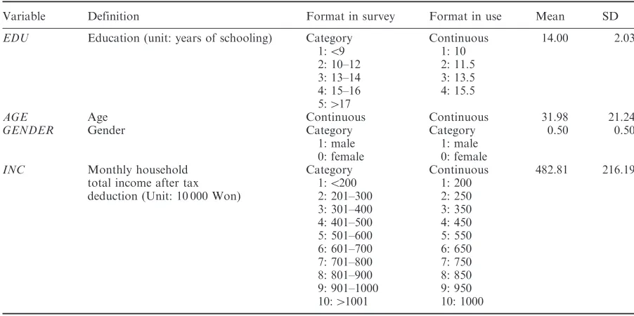
The ARAI’s obtained from this gamble experiment are used in the log-likelihood of RAM (Equation 17). Theex anteWTP for the service is assumed to be a linear function as
w&
i ¼"0þ"1EDUiþ"2AGEiþ"3GENDERi
þ"4lnINCiþ"i ð19Þ
where the covariates are explained in Table 3. The coefficient estimates of the WTP model (Equation 19) and the estimated mean value of the WTP’s of the respondents in the sample are reported in Table 4. The left column reports the TDM estimation results and the right column reports the RAM. It is disappointing to learn that most of coefficient estimates are not statistically significant except that of education level. Furthermore, it should be recognized that the WTP model of Equation 19 itself is also somewhat lacking as a model predicting how much a potential consumer is willing to pay for the service. However, the main purpose of this empirical study is not estimating the coefficients but demonstrating how much lower the TDM would estimate the WTP, and how important the risk premium is when estimating the WTP by using purchasing behaviour data. Even with a perfect model, an estimation process without considering the risk premium could not predict the WTP as precisely as would an estimation process that does so, if a consumer takes the risk premium into account when making a purchasing decision. What is impor-tant is not the RAM’s predictive power itself but its relative prediction superiority over TDM.
An initial basis of comparison can be made in terms of the distributions of the WTP obtained from TDM and RAM. Figure 1 presents the distribution of WTP estimates by the two mechanisms and the risk premiums. As expected, the mean of WTP estimates is much higher for the RAM than for the TDM. The difference reflects the risk premium the consumers are willing to pay for avoiding the uncertainties associ-ated with the new cell phone service.
Table 1. Percentage of ‘Yes’ votes by bid prices
Bid price (Won) Sample size
Percentage of
Table 2. Frequencies of the consumers’ risk premium for the game and absolute risk aversion index
Risk premium ARAI Frequencies
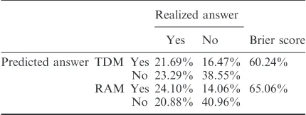
We may compare the two mechanisms in terms of binary prediction accuracies. The real binary answers (yes or no) given by respondents can be compared with the predicted binary answers made by TDM and RAM to see which mechanism predicts the real answer more accurately. According to each mecha-nism (Equation 2) and (Equation 6), the predicted answers of RAM are made by comparing the estimated WTP with the differently assigned bid price plus estimated risk premium while those of
TDM are made by comparing the estimated WTP with the differently assigned bid price only. There are four possible combinations of prediction and realiza-tion as presented in Table 5.
We find that the RAM makes a more accurate binary prediction than the TDM. The correct predic-tion ratio of RAM is 65.06% while that of TDM is 60.24%. Even though we cannot make a rigorous assertion, this provides support for the RAM being the purchasing decision mechanism for a new product Table 3. Definition and sample statistics of variables
Variable Definition Format in survey Format in use Mean SD
EDU Education (unit: years of schooling) Category Continuous 14.00 2.03
1:59 1: 10
2: 10–12 2: 11.5
3: 13–14 3: 13.5
4: 15–16 4: 15.5
5:417
AGE Age Continuous Continuous 31.98 21.24
GENDER Gender Category Category 0.50 0.50
1: male 1: male
0: female 0: female
INC Monthly household
total income after tax deduction (Unit: 10 000 Won)
Category Continuous 482.81 216.19
1:5200 1: 200
2: 201–300 2: 250
3: 301–400 3: 350
4: 401–500 4: 450
5: 501–600 5: 550
6: 601–700 6: 650
7: 701–800 7: 750
8: 801–900 8: 850
9: 901–1000 9: 950
10:41001 10: 1000
Table 4. Comparison of CVM/RAM with CVM/TDM
CVM/TDM CVM/RAM
Independent variables Estimates SE Estimates SE
WTP function
Constant 9524.38 9241.63 15 042.12 8581.47
EDU "809.45& 370.19 "658.11& 318.46
AGE 6.29 30.75 13.15 31.15
GENDER 1770.04 1298.95 415.01 1177.57
ln(INC) 860.87 1455.12 837.66 1308.59
!u 6765.98 1123.86
!" 7599.02 2126.83 6756.93 1725.80
Mean of WTP 4511 1804 11 552 1372
Median of WTP 4343 11 474
log likelihood "0.6484 "0.6145
Number of observations 249 249
having considerable performance uncertainty. Companies that are about to release a new product can use the RAM to make better demand predictions for each possible price.
V. Concluding Remarks
As Kalish (1985) notes, normally there is uncertainty with regard to a product’s experience attributes. This is especially true for nonmarket goods such as new products. So the actual value of the product to the consumer is not known for sure. A risk averse consumer will pay less for a risky choice in compar-ison with buying a product with a sure expected value. One expects the risk premium to result in lower demand at any price, the larger the degree of valuation uncertainty.
Much literature dealing with uncertainty in con-sumer purchasing decisions assumes a distribution of
WTP and ad hoc purchasing rules. An example is
Wang (1997) where a distribution for WTP and two arbitrary thresholds are assumed. However, no explanation is given regarding the location of the thresholds. In our approach, the thresholds can be determined by the risk premium.
Future research should examine the dynamics of how consumers adjust their risk premium over time. We conjecture that the risk premium for a really new product will decline over time as uncertainty
diminishes with experience and knowledge.
Marketers would be expected to change price levels accordingly.
References
Alberini, A., Boyle, K. and Welsh, M. (2003) Analysis of contingent valuation data with multiple bids: a response option allowing respondents to express
uncertainty,Journal of Environmental Economics and
Management,45, 40–62.
Ariely, D., Loewenstein, G. and Prelec, D. (2003) Coherent arbitrariness: stable demand curves without stable
preferences, Quarterly Journal of Economics, 118,
73–105.
Cameron, T. A. and James, M. D. (1987) Estimating willingness to pay from survey data: an alternative
pre-test-market evaluation procedure, Journal of
Marketing Research,24, 389–95.
Cameron, T. A. and Quiggin, J. (1994) Estimation using contingent valuation data from a dichotomous choice
with follow-up questionnaire,Journal of Environmental
Economics and Management,27, 218–34.
Carson, R. T., Hanemann, W. M., Kopp, R. J., Krosnick, J. A., Mitchell, R. C., Presser, S., Ruud, P. A. and Smith, V. K. (1994) Prospective interim lost use value
Fig. 1. Distribution of WTP and risk premium
Table 5. Prediction accuracies of TDM and RAM
Realized answer
Yes No Brier score
Predicted answer TDM Yes 21.69% 16.47% 60.24% No 23.29% 38.55% RAM Yes 24.10% 14.06% 65.06%
due to DDT and PCB contamination in the southern California Bight, A report of natural resource damage
assessment, Industrial Economics, NOAA,
Washington, DC.
Carson, R. T. and Mitchell, R. C. (1994)A Bibliography of
Contingent Valuation Studies and Papers, Natural
Resource Damage Assessment, Inc., La Jolla,
California.
Champ, P. A., Bishop, R. C., Brown, T. C. and McCollum, D. W. (1997) Using donation mechanisms to value
nonuse benefits from public goods, Journal of
Environmental Economics and Management,33, 151–62.
Chang, J.-I., Yoo, S.-H. and Kwak, S.-J. (2007) An investigation of preference uncertainty in the
contin-gent valuation study, Applied Economics Letters, 14,
691–5.
Cummings, R. G., Brookshire, D. S. and Schulze, W. D.
(1986)Valuing Environmental Goods: An Assessment of
the Contingent Valuation Method, Rowman and
Allanheld, Totowa, NJ.
Hanemann, W. M. and Kristro¨m, B. (1995) Preference
uncertainty, optimal designs and spikes, in Current
Issues in Environmental Economics (Eds)
P.-O. Johansson, B. Kristro¨m and K.-G. Ma¨ler,
Manchester University Press, Manchester, UK,
pp. 58–77.
Hanley, N., Kristro¨m, B. and Shogren, J. F. (2009) Coherent arbitrariness: on value uncertainty for
environmental goods,Land Economics,85, 41–50.
Johannesson, M., Liljas, B. and Johansson, P.-O. (1998)
An experimental comparison of dichotomous
choice contingent valuation questions and
real purchase decisions, Applied Economics, 30,
643–7.
Kalish, S. (1985) A new product adoption model with price,
advertising, and uncertainty,Management Science,31,
1569–85.
Malinvaud, E. (1985)Lectures on Microeconomic Theory,
North-Holland, New York.
Mauro, C. D. and Maffioletti, A. (2004) Attitudes to risk and attitudes to uncertainty: experimental evidence,
Applied Economics,36, 357–72.
Paradiso, M. and Trisorio, A. (2001) The effect of knowledge on the disparity between hypothetical and
real willingness to pay, Applied Economics, 33,
1359–64.
Ready, R. C., Whitehead, J. C. and Blomquist, G. (1995) Contingent valuation when respondents are
ambiva-lent, Journal of Environmental Economics and
Management,29, 181–96.
Van Kooten, G. C., Krcmar, E. and Bulte, E. H. (2001) Preference uncertainty in non-market valuation: a
fuzzy approach, American Journal of Agricultural
Economics,83, 487–500.
Wang, H. (1997) Treatment of ‘Don’t know’ responses in contingent valuation surveys: a random valuation
model, Journal of Environmental Economics and
Management,32, 219–32.
Wertenbroch, K. and Skiera, B. (2002)
Measuring consumers’ willingness to pay at the point
of purchase, Journal of Marketing Research, 39,